Volume 4, No. 2, Jan-Feb 2013
International Journal of Advanced Research in Computer Science
CASE STUDY AND REPORT
Available Online at www.ijarcs.info
ISSN No. 0976-5697
Optimal Solution Strategy for University Course Timetabling Problem
Chacha Stephen
Department of Mathematics, Private Bag, Mkwawa University College of Education, Iringa, Tanzania
Allen Rangia Mushi*
Department of Mathematics, Box 35062, University of Dar es salaam, Tanzania
Abstract— This paper describes formulations of the University Course Timetabling Problem as used at Mkwawa University College of Education. University Course Timetabling is the Problem of scheduling resources such as lectures, courses and rooms to a number of timeslots over a planning horizon, normally a week, while satisfying a number of problem-specific constraints. In this study, we have developed three models and tested using real data from the stated University. It has been possible to get optimal solution for real problem instances through reformulations of models which involve a mixture of binary and time-indexed variables.
Keywords- Timetabling Problem, Combinatorial Optimization, NP-hard problem, reformulations, scheduling.
I. INTRODUCTION
University Course Timetabling Problem (UCTP) refers to the allocation of University courses to given resources being placed in space time, in such a way as to satisfy a set of desirable objectives as much as possible [1]. Course timetabling specifically involves assigning courses to teachers and classrooms, as well as the teacher student and meeting times in days. Given the increasing number of student’s enrolment in Tanzanian Universities, a large number of courses are offered every semester. Each course has varying number of enrolled students who registers for different courses that are shared among programmes. Furthermore, classrooms are always scarce, which complicates the assignment of courses to classrooms.
Two common techniques for solving timetabling problems are exact and heuristics. Exact methods include formulating and solving mathematical programming models. For large problems, it could be difficult to find and prove the existence of an optimal solution, within short computing times [2]. This follows from the fact that the problem is known to be NP-Hard i.e. no optimal algorithm is known for the solution of a general such problem within reasonable time. Consequently, many efforts have concentrated in developing heuristics in order to find a good solution within a reasonable amount of time. Some heuristic approaches for solving the course timetabling problem were proposed in (e.g. [3], [4] and [5]). However, exact approaches have provided optimal solutions to some specific cases. They have also provided benchmarks for testing the performance of heuristic procedures. One of applications of exact methods includes [6].
This is also an extension of the basic mathematical programming model proposed in [7] in which it is shown that timetabling problems with data sizes comparable to that of some real institutions can be solved with the help of the proposed basic model. Tripathy [8] presents a large integer linear program to determine room and time allocations for graduate courses where students, subjects and rooms are grouped into appropriate categories in order to reduce the problem to a manageable size. A Lagrangean relaxation procedure in conjunction with sub gradient optimization to compute the multipliers is used to solve the problem. A
two-stage multi-objective 0-1 course scheduling model is proposed in [9]. Birbas et al [6] formulated a binary integer program to determine the weekly timetable for Greek high schools where, for each class-section, a sequence of courses to be taught on every day of the week must be determined. Dimopoulou and Miliotis [10] and Papoutsis [11] employ a column-generation approach to solve 0-1 timetabling problem for Greek schools and presented some good results in their case study. Mushi [12] shows the existence of various models for timetabling problem by using integer programming where the quality of a model depended on the closeness of the problem to the integer polytope. University of Dar es salaam was used as a case study. Al-Yakoob and Sherali [13] adopted a Mixed-Integer Programming approach to determine timeslots for courses at Kuwait University. Schedule Expert is a system that was developed by [4], and uses a 0-1 mathematical model to schedule courses at the Cornell University School of Hotel Administration.
There are often different ways of mathematically representing the same optimization problem. Obtaining an optimal solution to a large integer programming problem in a reasonable amount of computer time may well depend on the way it is formulated. Much recent research has been directed towards the reformulation of integer programming problems. In this regard, it is sometimes advantageous to increase (rather than decrease) the number of integer variables, the number of constraints or both. Discussions of alternative formulation approaches are given in [14] and [15]. More recent work is presented by G. Lach and M.E. Lubbecke in which they formulated and solved Integer Programming model for curriculum-based course timetabling problem for Udine Benchmark test data [16]. Since the UCTP structures are not standard as they vary from one institution to another, most of the presented research findings are addressing specific case studies.
II. COURSE TIMETABLING AT MUCE
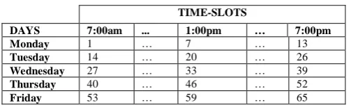
[image:2.595.29.281.185.262.2]MUCE being a young fast growing institution, it consists of 3,000 students (from 1st to 3rd year), 150 lecturers, 19 lecture and seminar rooms excluding laboratories. Currently there are a total of 95 courses offered in all faculties, that is Science, Humanity and Education. The timetable starts from 7:00am and ends at 7:00pm, and repeats for five working days (Monday to Friday), making a total of sixty five time slots.
Table I:MUCE Timetable Layout
TIME-SLOTS
DAYS 7:00am ... 1:00pm … 7:00pm
Monday 1 … 7 … 13
Tuesday 14 … 20 … 26
Wednesday 27 … 33 … 39
Thursday 40 … 46 … 52
Friday 53 … 59 … 65
Table I shows a typical layout of timeslots at MUCE. Timetabling constraints are normally divided into hard and soft. Hard constraints ought to be respected while soft constraints are to be satisfied as much as possible. Constraints at MUCE’s course timetable are as follows;
A. Hard Constraints:
A feasible timetable is one in which all courses have been assigned a timeslot and a room, so that the following hard constraints are satisfied;
(i) No student attends more than one course at the same time;
(ii) The assigned room is big enough for all the attending students and possess all the features required by the course;
(iii)Only one course is taking place in each room at a given time.
(iv) No lecturer is assigned more than one course in the same timeslot
B. Soft constraints:
We need to minimize the use of the following timeslots; (i) Early morning timeslots due to cold and distant off
campus students and lecturers,
(ii) Lunch timeslots to allow for lunch breaks,
(iii)Friday afternoon slots to allow for Muslims prayers from 12 noon to 2 pm and seventh day Adventist worshippers starting from 18 hours.
Note that, some students and lecturers may prefer morning sessions to evening ones and vice versa, therefore, soft constraints cannot always be satisfied, they can only be treated to reasonable state and in a fairly way possible by minimizing violations as much as possible. As pointed earlier, a timetable is said to be feasible if it satisfies all the hard constraints. The objective is to minimize the number of soft constraint violations in a feasible timetable. The mathematical programming formulations for this problem are of the form;
Minimize: Subject to.
Where is the solution vector and is the objective function. The objective function in this case will represent all soft constraints and contains all hard constraints.
Many formulations are possible for these problems, and therefore analysis of their performances and the upper limit
on problems sizes are discussed. For instance the choice of the solution vector representation could be integral, mixed integer, binary, time indexed and many others. These choices have implications to the formulations and properties of the associated model. Three models are developed in this paper with different features and compare their performances as presented in the next section.
III. MATHEMATICAL FORMULATIONS
We define the following structures;
Sets:
Set of timeslots Set of rooms
Set of Courses Set of classrooms Decision Variables
Parameters
=
Note that, two courses collide if they have students or lecturers in common. The matrix M is called a ‘conflict matrix’ and is used to detect collisions between courses. Tm Maximum number of timeslots for MUCE timetable,
N Total number of courses at MUCE, Total number of rooms at MUCE,
1
λ
Weight given to morning timeslots,
2
λ
Weight given to lunch timeslots,3
λ
Weight given to Friday afternoon timeslots,A. Model 1: A Single 0/1 variable:
This model uses full binary variables for decision making. Although they tend to create large variable set models, their inherently sparse matrices could sometimes be easily solved. Constraints of the resulting model are therefore represented as follows;
a. Hard Constraints:
(i) Course Collisions:
This constraint ensures that there is no course collision i.e. no courses with common students or common lecturer is scheduled in the same timeslot. The conflict is detected from the conflict matrix as follows;
, for all and all This enforces the fact that for any pair of courses where , if there is a collision (i.e. ), then the two courses cannot be scheduled in the same time slot, .
(ii) Room size violations:
Where refers to the size of room and is the capacity of course
(iii) Room collisions:
Two courses should not be allocated in the same room r at the same timeslot k
(iv) Courses assignment:
for all .
This ensures that each course is slotted and assigned one room.
b. Soft constraints:
As pointed earlier, soft constraints are associated with time desirability and we have the following soft constraints;
(i) Minimize early morning sessions due to cold and distant residence off campus, both for students and lecturers,
Let = the early morning slots, then,
Minimize
Where counts the number of times the morning slots have been violated.
(ii) Make lunch hours as free as possible,
Given = the lunch hours, then,
Minimize
Where Counts the number of times the lunch hours have been violated.
(iii)Minimize the religion timeslots;
Let = religion timeslots, then,
Minimize
c. Objective function:
Objective function is a linear combination of the soft constraints, making a function of the form
, where λ is constant which is given a weight depending on the importance of the associated constraint in relation to others. This weight is normally determined from the experience of the scheduler and other stakeholders of the timetabling system.
From the objective function and hard constraints we have to;
Minimize:
Subject to:
(a). , and all
(b).
(c). 1for all
(d). for all
(e). , , and
.
Given a timetable with C courses, R rooms, and T timeslots, we have a problem with CRT variables. A typical Course timetable at MUCE involves 95 courses, 19 rooms, 3,000 students and 160 Lecturers on a 65 slots time interval. This gives a problem with CRT= 95×65×19= 117,325variables. The problem was too big to solve by common Mathematical Programming software available to us. We attempt to minimize the number of variables by breaking the variable definition into two separate sets of variables. This gives the second model as presented below;
B. Model 2: Two 0/1 variables:
In this case we break the decision variable into two as follows:
Let,
The problem constraints are divided into hard and soft as stated in the previous model and are now modelled as follows:-
a. Hard Constraints:
(i) Course collision:
Courses
i
1 andi
2 cannot be allocated to the same timeslot k ifThat is;
, either or or both, thus; or
(ii) Room size:
Total students registered for course ‘ ’ should not exceed the corresponding room capacity ,
Mathematically, written as
(iii) Room collision:
Two courses and should not be allocated in the same room at the same timeslot. Note that, two courses may be in the same timeslot but in different rooms.
Thus if then 1 and vice
versa
We have therefore;
, for all such that
(iv) Each course must be assigned a room and a timeslot:
For each course, the sum of all timeslots must be 1 (assigned exactly once)
, for all courses
i
(v) For each course, the sum of all rooms must be 1 (assigned exactly once)
, for all courses
i
b. Soft constraints:
(i). Minimizing the use of the first sessions due to cold and distant residence off campus;
Minimize
(ii).Making lunch hours (slots) as free as possible; Minimize =
(iii).Minimizing the use of religion priority hours;
Minimize
c. Objective function:
+ +
Then complete model becomes;
Minimize + +
Subject to (a).
(b). .
(f). , ,i∈C,k∈1..Tm and r∈R. In this model we have C (T+R) = 95(65+19) = 7,980 variables. This is a considerable reduction from the previous model. However, the number of variables is still high to be able to solve a real timetable problem with software that is available to us. The number of variables can be further refined if we minimize the number of 0/1 variables by reformulation from model 2. This prompted the formulation of mixed pure integer (time-indexed) and 0/1 variables as shown in the next model.
C. Model 3: Combined Time-indexed and binary variables Let;
= Timeslot of course i
, if course i is slotted in room
r
and 0 otherwise = number of students in course i=Capacity of room
r
a. Objective function:
+ +
b. Constraints:
(i) Enforcing : That is, if then which can be modeled as follows;
,
Where N is a sufficiently large value (in this case we take the value of the largest timeslot number, which is 65). Note that, if then , which implies that .
(ii) Enforcing : that is if ; this is modeled as follows;
, for all
Note: if then .
(iii) Course collision: , for all
Note: if then that is
(iv) Room size:
, for all i and
r
. (v) Room collision:If and then we must have , and is modeled as follows;
, for all
i
1≠
i
2Note: when and , then, .
We would then like to have a constraint of the form;
, that is, , then must be zero.
In this model we have reduced the number of variables to 1,965 and fortunately the used solver (GLPK-Solver) can accommodate this number of variables.
The complete model 3 is therefore as follows; Minimize:
+ +
Subject to:
a. , where N is 65
b. , for all
i
1≠
i
2c. , for all
i
andr
,d. , for all , where
e. , for all
IV. SUMMARY OF RESULTS
This section presents a summary of results for the three models. Tables below summarize parameters, data and results as discussed in the previous sections;
Table2: Summary of Results for model 1 (single 0/1 variable)
No.
Si
z
e
(n)
Ro
ws
C
o
lum
ns
No
n
-ze
ro
s:
O
b
je
c
ti
v
e
T
im
e
(S
e
cs
)
1 5 5,001,811 6,175 485,640 0 1.0
2 10 2,235,361 12,350 2,784,260 0 7.3
3 15 - - - - Too big
This model managed to run and gave results for up to
n=10 as shown in Table II. The number of rows is
exponentially increasing with the value of n, where n is the number of courses. It is worth noting that the underlying matrix is sparse with many zeros, but still the solution is hard to find for a sizeable problem. Time spent is rather small for the solved problem, but drastically increases with a slight increase in size of n. This is typical of NP-Hard problems which are normally exponential, and therefore difficult to solve to optimality.
It was observed that the searching space can be reduced by dividing it into regions for some constraints. For instance, a constraint that involves searching throughout the course combinations for course conflicts can be reduced to half. This steams from the fact that the collision matrix is symmetric and therefore only suffices to search in one triangle, either upper or lower. Furthermore, it was observed that some constraints require exclusion of the cases where courses are equal, since they don’t bring any new information or constraint. These reformulations on the bounds of constraints in model 1 resulted into a summary shown in Table III.
Table II: Result summary of model 1 for i1≠i2 and i2>i1.
Si
z
e
(n)
Rows Columns objective Time (secs)
i1 ≠i2 i2>
i1
i1 ≠i2 i2>
i1
i1 ≠i2 i2>
i1
i1 ≠i2 i2>
i1
5 5,001,
81
1
253,
18
1
6,
175 6,175 0 0 1.0 0.7
10 2,
235,
36
1
1,
123,
86
1
12,
350
12,
350
0 0 7.3 3.1
15 - 2,
612,
04
1
- 18,
525
- 0 Too
From Table III, the number of constraints is reduced to almost half of its original values. That is, number of rows for is approximately twice the number of rows for the model solved using . However, this did not improve performance, as only problems up to size n=10 could be solved to optimality. This indicates that reduction of constraints does not necessarily improve performance since it may not necessarily reduce the polyhedron associated with the specific problem.
Next, we show results for model 2 which divides the decision variable into two components. This is still a purely 0/1 variable model, but the division of the decision variable is expected to cut-off considerably the number of variables and possibly reduce infeasibilities in the resulting polyhedron.
Table 4: Summary of Results for model 2
[image:5.595.309.557.232.416.2]After reduction of problem size in terms of constraints and decision variables, the formulated model has been able to solve problems up to size n=41 as shown in Table IV. This is a considerable improvement over the previous model where only the size n=10 was possible. The highest time used was 253 seconds which is just over four minutes, a quite tolerable time. This indicates that, further reformulations may result into a model which could actually solve a realistic timetabling instance to optimality. Further reformulation by grouping the searching space as it was done in the previous model was implemented and the summary of results is as shown in Table V.
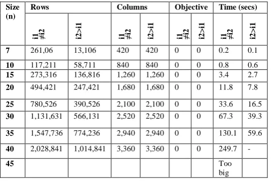
Table 5: Result summary of model two for i1≠i2 and i2>i1
Size (n)
Rows Columns Objective Time (secs)
i1 ≠i2 i2>
i1
i1 ≠i2 i2>
i1
i1 ≠i2 i2>
i1
i1 ≠i2 i2>
i1
7 261,06 13,106 420 420 0 0 0.2 0.1
10 117,211 58,711 840 840 0 0 0.8 0.6
15 273,316 136,816 1,260 1,260 0 0 3.4 2.7
20 494,421 247,421 1,680 1,680 0 0 11.8 7.8
25 780,526 390,526 2,100 2,100 0 0 33.6 16.5
30 1,131,631 566,131 2,520 2,520 0 0 67.3 39.3
35 1,547,736 774,236 2,940 2,940 0 0 130.1 59.6
40 2,028,841 1,014,841 3,360 3,360 0 0 249.7 -
45 Too
big
The same trend as in the previous model is observed, where despite of reduction in searching space, there is no improvement in the performance. If anything, the size n=40 could not obtain a solution within reasonable time. This was solved in four minutes in the un-reformulated model 2. Again, it signifies the fact that a good model does not necessarily result from reduction of problem size.
Previous studies have shown that, time indexed formulations coupled with binary variables can provide good models [12]. Note that, it may not be possible to avoid binary variables all-together, since they are needed in specifying various decisions situations. Model 3 is designed to combine these variables and the results are presented in Table VI.
Table 6: Results summary for model 3
S
ize
(n
) Rows Columns
O
bj
T
im
e
(S
e
cs
)
5 636 (435 integer, 335 binary) 0 0
10 1,796 (895 integer, 695 binary) 0 0.1
20 5,691 (1,890 integer, 1,490 binary) 0 0.4
30 11,686 (2,985 integer, 2,385 binary) 0 1.1
40 19,781 (4,180 integer, 3,380 binary) 0 3.9
50 29,976 (5,475 integer, 4,475 binary) 0 8.9
60 42,271 (6,870 integer, 5,670 binary) 0 23.6
70 56,666 (8,365 integer, 6,965 binary) 0 615.7
80 73,161 (9,960 integer, 8,360 binary) 0 122.7
85 82,196 (10,795 integer, 9,095 binary) 0 871
90 91,756 (11,655 integer, 9,855 binary) 0 894.2
95 101,841 (12,540 integer, 10,640binary) 0 1,160.2
This model managed to solve the whole of MUCE timetabling problem by securing an optimal solution to the problem of size n=95, which is the total number of courses at MUCE. This formulation therefore means that it provides a better polyhedron by starting with a model which is closer to the required polytope than the previous models. This solution was found after 1,160 seconds which is more than 19 minutes. The time is tolerable for timetabling problems and is not strange for optimal solution algorithms.
V. CONCLUSIONS AND FUTURE RESEARCH
In this research, we developed an algorithm for UCTP and use Mkwawa University College of Education as a case study, where exact approach was employed (mixed integer programming). All three models were solved to optimality, however models 1 and 2 were only solved for small instances. This is expected since the problem is NP-Hard and therefore the solution space is expected to grow exponentially with the size n.
Fortunately, reformulation of the previous models made it possible to solve a real problem instance to optimality. Although this is not a guarantee that all future instances would be solved to optimality through the formulation, it provides a good benchmark for future research in the problem.
A. Future Research Directions:
In this study we have applied exact techniques to solve the UCTP at MUCE. As MUCE grows, there is a need to apply state of the art global heuristic techniques. Furthermore, this study considered only a few time
Si
z
e
(n)
Rows Columns Objective Time
(Secs)
5 26,106 420 0 0.2
10 117,211 840 0 0.8
15 273,316 1,260 0 3.9
20 494,421 1,680 0 11.8
25 780,526 2,100 0 33.6
30 1,131,631 2520 0 67.3
35 1,547,736 2,940 0 130.1
40 2,028,841 3,360 0 249.7
41 2,132,862 3,444 0 253.6
[image:5.595.25.294.608.788.2]restrictions on soft constraints. Other soft constraints exist such as teacher and student preferences and the need to spread courses over the week. It is worth considering addition of as many soft constraints as possible so as to improve the quality of solution. Exact approach can still be extended with further reformulations and development of deepest-cut constraints (facets) which defines the problem’s polytope ([17], [18]).
VI. REFERENCES
[1] A. Wren, Scheduling, Timetabling and Rostering, A Special Relationship? In the Practice and Theory of Automated Timetabling, ed. Springer- Verlag, pp. 46-75,1996.
[2] D. Costa, A Tabu Search Algorithm for computing an operational timetable, European Journal of Operational Research, vol.76, pp 98-110, 1994.
[3] J. Aubin, and J.A. Ferland, A large scale timetabling problem, Computers and Operations Research, vol.16, pp. 67-77, 1989. [4] R. Hinkin, and M. G. Thompson, SchedulExpert, Scheduling
Courses in the Cornell University, School of Hotel Administration, Ithaca, New York, vol. 32, pp. 45–57, 2002. [5] M. Wright, School timetabling using heuristic search. The
Journal of the Operational Research Society, vol.47, pp 347-357, 1996.
[6] T. Birbas, S. Daskalaki and E. Housos, Timetabling for Greek high schools, Journal of the Operational Research Society, vol.48, pp. 1191-1200,1997.
[7] A. Gunawan, K.M. Ng, K.L Poh, A Mathematical Programming model for a Timetabling Problem, Proceedings of the International Conference on Scientific Computing, Navade, USA, 2006.
[8] A. Tripathy, School Timetabling, a Case in Large Binary Integer Linear Programming, Management Science, vol.30, pp. 1473-1489 1984.
[9] M.A. Badri, A two-stage multi-objective scheduling model for faculty-course time assignments. European Journal of Operational Research, vol.94, pp16-28, 1996.
[10] M. Dimopoulou and P. Miliotis, Implementation of a University Course and Examination Timetabling System, European Journal of Operational Research, vol.130, pp.202-213, 2001.
[11] K. Papoutsis, C. Valouxis and E. Housos, A column generation approach for the timetabling problem of Greek high schools, Journal of the Operational Research Society, vol. 54, pp. 230-238, 2003.
[12] Mushi, A.R, Mathematical Programming Formulations for the Examinations Timetable Problem, The case of the University of Dar es salaam, African Journal Science and Technology (AJST), Science and Engineering Series, vol.5, pp. 34-40, 2004.
[13] S.M. Al-Yakoob and H.D. Sherali, A mixed-integer programming approach to a Class timetabling problem: A case study with gender policies and traffic considerations. European Journal of Operational Research, 180(3): pp1028-1044, 2007.
[14] M. Guignard and K. Spielberg, Logical reduction methods in zero one programming; minimal preferred variables, Operations Research, vol.29, pp.49-74, 1981.
[15] H.P. Williams, Model building in mathematical programming, 2nd Ed. Wiley, New York, 1985.
[16] G. Lach and M.E. Lubbecke, Curriculum Based course timetabling: New solution to Udine benchmark instances, Annals of Operations Research, Springer, Vol. 194 (1), pp 255-272, 2012.
[17] Grotschel M. Junger M. & Reinelt G. A Cutting Plane Algorithm for the Linear Ordering Problem, European Journal of Operations Research, 6(1984), 1195-1220. [18] Crowder, H, Johnson, E.L and Padberg, M, Solving