Passive RFID Rotation Dimension Reduction via Aggregation

(1)

University of Windsor University of Windsor

Scholarship at UWindsor

Electronic Theses and Dissertations Theses, Dissertations, and Major Papers

2017

Passive RFID Rotation Dimension Reduction via Aggregation

Eric Matthews University of Windsor

Follow this and additional works at: https://scholar.uwindsor.ca/etd

Recommended Citation Recommended Citation

Matthews, Eric, "Passive RFID Rotation Dimension Reduction via Aggregation" (2017). Electronic Theses and Dissertations. 5998.

https://scholar.uwindsor.ca/etd/5998

This online database contains the full-text of PhD dissertations and Masters’ theses of University of Windsor students from 1954 forward. These documents are made available for personal study and research purposes only, in accordance with the Canadian Copyright Act and the Creative Commons license—CC BY-NC-ND (Attribution, Non-Commercial, No Derivative Works). Under this license, works must always be attributed to the copyright holder (original author), cannot be used for any commercial purposes, and may not be altered. Any other use would require the permission of the copyright holder. Students may inquire about withdrawing their dissertation and/or thesis from this database. For additional inquiries, please contact the repository administrator via email

(2)

Aggregation

By:

Eric Matthews

A Thesis

Submitted to the Faculty of Graduate Studies through the School of Computer Science in Partial Fulfillment of the Requirements for

the Degree of Master of Science at the University of Windsor

Windsor, Ontario, Canada

2017

(3)

Passive RFID Rotation Dimension Reduction via

Aggregation

by

Eric Matthews

APPROVED BY:

W. Kedzierski Department of Physics

R. Kent

School of Computer Science

R. Maev, Co-Supervisor Department of Physics

R. Frost, Co-Supervisor School of Computer Science

(4)

I hereby certify that I am the sole author of this thesis and that no part of this thesis has

been published or submitted for publication.

I certify that, to the best of my knowledge, my thesis does not infringe upon anyone’s

copyright nor violate any proprietary rights and that any ideas, techniques, quotations, or

any other material from the work of other people included in my thesis, published or

oth-erwise, are fully acknowledged in accordance with the standard referencing practices.

Fur-thermore, to the extent that I have included copyrighted material that surpasses the bounds

of fair dealing within the meaning of the Canada Copyright Act, I certify that I have

ob-tained a written permission from the copyright owner(s) to include such material(s) in my

thesis and have included copies of such copyright clearances to my appendix.

I declare that this is a true copy of my thesis, including any final revisions, as approved

by my thesis committee and the Graduate Studies office, and that this thesis has not been

submitted for a higher degree to any other University or Institution.

(5)

Abstract

Radio Frequency IDentification (RFID) has applications in object identification, position,

and orientation tracking. RFID technology can be applied in hospitals for patient and

equip-ment tracking, stores and warehouses for product tracking, robots for self-localisation,

tracking hazardous materials, or locating any other desired object. Efficient and accurate

algorithms that perform localisation are required to extract meaningful data beyond simple

identification. A Received Signal Strength Indicator (RSSI) is the strength of a received

radio frequency signal used to localise passive and active RFID tags. Many factors affect

RSSI such as reflections, tag rotation in 3D space, and obstacles blocking line-of-sight.

LANDMARC is a statistical method for estimating tag location based on a target tag’s

sim-ilarity to surrounding reference tags. LANDMARC does not take into account the rotation

of the target tag. By either aggregating multiple reference tag positions at various

rota-tions, or by determining a rotation value for a newly read tag, we can perform an expected

value calculation based on a comparison to the k-most similar training samples via an

al-gorithm called K-Nearest Neighbours (KNN) more accurately. By choosing the average as

the aggregation function, we improve the relative accuracy of single-rotation LANDMARC

localisation by 10%, and any-rotation localisation by 20%.

(6)

I would like to thank, in no particular order:

Dr. Richard A. Frost, with whom I have been working since the second year of my

undergraduate degree at the University of Windsor. He has guided me throughout my

Master’s, and has provided me with many opportunities to learn. He inspires my continued

interest in natural language processing, and functional programming.

Dr. Roman G. Maev, with whom I have been working since the beginning of my

Mas-ter’s degree. I would like to thank him for the opportunity to be involved with the RFID

project, and for his assistance with my thesis.

Dimiry Gavrilov, who I have closely worked with throughout my Master’s degree. He

has taught me many physics related concepts associated with our research, and has assisted

me throughout my Master’s education.

My Internal and External Readers, Dr. Robert Kent, and Dr. Wladyslav Kedzierski for

being available to participate as part of my Thesis Committee.

Shane Peelar for giving me advice during my thesis, and Bryan St. Amour and Paul

Preney for letting me use their LA_TEXstyles.

All of the secretaries in the School of Computer Science for their support during my

de-gree. Their assistance was vital to my organization, and ability to meet deadlines

through-out my degree.

(7)

Acronyms

2D Two Dimensional.

3D Three Dimensional.

ANN Artificial Neural Network.

AoA Angle of Arrival.

ASK Amplitude Shift Keying.

CPU Central Processing Unit.

EPC Electronic Product Code.

GPS Global Positioning System.

ID Identification.

KNN K-Nearest Neighbours.

LANDMARC LocAtioN iDentification based on dynaMic Active Rfid Calibration.

LMMSE Linear Minimum Mean Square Error.

ML Machine Learning.

MMSE Minimum Mean Square Error.

MSE Mean Square Error.

OOK On-Off Shift Keying.

PL Path Loss.

RBF Radial Basis Function.

RBFNN Radial Basis Function Neural Network.

(10)

RDA Rotation Dimension Abstraction.

RDR Rotation Dimension Reduction.

RF Radio Frequency.

RFID Radio Frequency IDentification.

RSSI Received Signal Strength Indicator.

(11)

List of Figures

2.1 Linear polarization depicted by [32]. . . 8

2.2 Orientation with reduced gain efficiency for linear polarization [21]. . . 9

2.3 Circular polarization on the same tag orientations as Figure 2.2 [21]. . . 9

2.4 A graph of distance vs path loss with and without reflections by [14]. . . 11

3.1 Visualization of LANDMARC by [Ni 2004] . . . 21

3.2 Depicting an example of the types of tag rotation [7]. . . 23

4.1 Graph of how rotation on each axis affects RSSI value in an anechoic cham-ber as researched by [7]. . . 29

5.1 A 4 meter by 4 meter LANDMARC grid trained at 8 different rotations. . . 35

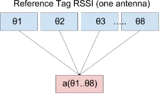
5.2 An example of dimension reduction on a reference tag’s RSSI at one an-tenna, with 8 different rotations. . . 38

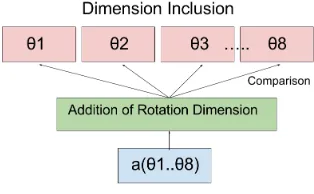
5.3 An example of dimension abstraction on a newly read test tag with a single rotation, and comparison function on reference tags at multiple rotations. . . 39

7.1 Features of the distance error distribution for LANDMARC using rotation dimension reduction, as well as various grid rotations relative to the target tag’s true rotation. . . 53

7.2 This is a comparison of the distance error distribution of estimated positions from the center of the LANDMARC grid. The true average distance from the center for our 421 samples was 1.7 meters. . . 54

7.3 The passive RFID tag that we have used in our experiments [33]. . . 55

7.4 The passive RFID antenna that we have used in our experiments [4] [30]. . . 55

7.5 The passive RFID antenna router that we have used in our experiments [31]. 55

(12)

Appendix A - Additional Results . . . 53

Appendix B - Equipment . . . 55

(13)

Chapter 1 Thesis Layout

The Problem

Radio Frequency IDentification (RFID) localisation has many challenges described

in Section 3.4. It is the goal of localisation algorithms, most of which are described in

Section 3.3, to overcome these challenges to improve the accuracy of estimated tag

loca-tions. RFID tag Received Signal Strength Indicator (RSSI) values fluctuate based on the

path of the signal from and back to the antenna. Rotating an RFID tag changes the pathloss

described in Section 2.4. We expand on this rotation fluctuation problem and how it affects

localisation in Section 4.2.

Importance

It is important to solve localisation problems to improve the accuracy of

localisa-tion algorithms. By improving the accuracy of said algorithms, applicalocalisa-tions such as those

discussed in Section 3.2 can more accurately fulfill their purpose, thereby improving the

performance of their application.

(14)

Previous Solutions

We discuss previous solutions in Section 4.4 where additional sensors, as well as

moving antennas, have solved the rotation challenge. These algorithms and applications

utilize additional sensors or additional system complexity to solve the problem, whereas we

aim to utilize only pre-existing information of an RFID localisation system with stationary

antennas.

New Solution

Our solution to improving machine learning algorithms on inconsistent sinusoidal

data involves reducing the dimension of the sinusoidal training data via an aggregation

function. This reduction allows a more accurate comparison between a newly read sample

at a specific instance of the sinusoid function. An example would be sampling the tide at

a single unknown time t while the tide follows a periodic function of t. This process is

described in Section 5.2.

Thesis Statement

For any dataset that contains a periodic dimension for which newly gathered

in-stances exist at only one unknown value within the period, we can improve the accuracy of

distance comparisons between such newly read instances and training data by reducing the

dimension of the training data via an aggregation function.

Originality

State of the art localisation algorithms seldom discuss the orientation of the passive

RFID tags that they wish to localise. Our solution uniquely considers solely the pre-existing

information in an RFID localisation system to solve the challenge that tag rotations

(15)

Chapter 1. Thesis Layout 3

Non-Triviality

It is logical to hypothesize that single-orientation localisation with both training and

target tags at solely the same orientation serves as a lower bound on localisation distance

error, since the rotation challenge has been removed from the system. We have found that

this is not the case. We first aggregate the RSSI of incorrect rotations into our training data.

We then use the aggregated data to perform localisation with an increased accuracy relative

to systems with no rotation solution. This process is shown in Section 5.2.

Proof

We demonstrate our thesis empirically by performing a localisation algorithm called

LANDMARC on a variety of rotational data. The results of our experiment are shown in

Section 6.3. We explain our performance increase by testing the accuracy of the K-Nearest

Neighbours algorithm used by LANDMARC. Our results for the K-Nearest Neighbours

comparison are shown in 5.4.

Explanation

We explain in 5.4 that our improvement in accuracy is because each RSSI at a single

ro-tation has inherent noise due to the walls and objects in an enclosed environment. Since

any one rotation may be unreliable, we aggregate the information of multiple different

ro-tations to reduce the noise that exists at a singular rotation. This results in more accurate

comparison, and therefore improved accuracy.

Other Discplinary Uses

This thesis applies to applications that use training data of a sinusoidal nature. It

allows for more accurate comparison of newly read samples that can only exist at a single

value within that sine wave, where noise may exist. Examples of such data are tidal shifts,

(16)

Conclusion

By using Rotation Dimension Reduction on LANDMARC training data, we have

aggregated the training data in the rotation dimension to allow for more accurate

compari-son of newly read samples. This has improved our LANDMARC localisation accuracy by

20% in the general case, and by 10% in a perfect rotation prediction system. Future work

includes analyzing such factors as the material of the object to which a tag is attached,

the effect of different aggregation functions, and the possibility of including other rotation

(17)

Chapter 2 Radio Frequency Identification

Radio Frequency IDentification (RFID) is the product of radar - discovered in 1935

- used during World War II to detect war planes at a far distance. Although no

identifica-tion capabilities existed to distinguish friendly from foe planes, according to [22] German

pilots would roll their planes, which would change the reflected radio signal. This allowed

the crews on the ground to perform vague identification. This is thought to be the first

application of RFID. Various research was conducted throughout the 1950s and 1960s with

published works on how radio waves could be used to identify objects. Commercial

ap-plications, such as stores, still use transponder technology that indicates whether or not an

item has been paid for. Patents started to be issued for applications in transponders in the

1970s, when the United States government started to develop RFID systems.

An RFID system can obtain the strength of a signal detected by a transceiver. Physics

equations can be used to estimate a distance between a transceiver and a signal, but with

modern computers we can also utilize algorithms that can compute an estimated position

for the source of a signal. Estimating the position of a signal source is important because of

the source of signal is physically attached to an object and follows the object’s movements,

then this position estimate for the signal’s source is also an estimate for the object on which

the signal source is attached. This allows the tracking of an object, useful for a variety of

applications.

(18)

2.1 Object Identification via Unique Code

RFID systems allow the identification of any object onto which an RFID tag is

placed. RFID tags are small metal tags that consist of a peice of memory than can be

written to and read from using radio frequency waves. These waves can operate at a variety

of frequencies, most of which are designated for general purpose short-range

communica-tion. By modulating a unique code into the signal, a receiving antenna can demodulate the

signal to determine which tag was read. The tags, along with one or more antennas form a

general purpose object identification and tracking system for use in various applications.

Barcodes are an example of another object identification technology. Even though

barcodes are prominently used in industry, RFID offers industry more features than

bar-codes at a slightly higher cost. Barcode technology utilizes lasers, and therefore requires a

reader to have line-of-sight vision of its target as described by [13], and according to [25]

has a short range at which a reader can identify the barcode - up to a few feet. Conversely,

even though line-of-sight is useful for RFID, radio waves can pass through certain objects,

and reflect around them, meaning that line-of-sight is no longer important. As well, radio

waves have a greatly increased range over the resolution of most laser optic readers used

in barcodes. However, RFID tags are more expensive than barcodes, but are reusable.

Bar-codes can be printed for as cheap as the ink costs to print them, and therefore disposed of

cheaply. RFID tags require specific cuts of metal, making it more expensive, and

there-fore important to retain every tag. Therethere-fore, in applications such as grocery stores, where

packaging is often disposed of, RFID tags could prove to be too expensive to be practical.

2.2 Active and Passive Tags

Passive RFID, patented in the United States in 1975 under Patent US4023167, and

later extended in 1986 under Patent US4688026, is a technology described to identify

metallic tags using a radio frequency antenna. According to the patents, if the antenna

is sufficiently close to the tag, meaning the Radio Frequency (RF) Signals can hit the tag

(19)

Chapter 2. Radio Frequency Identification 7

burst. It then modulates this signal, thereby changing the amplitudes of the electric wave,

using an on-board circuit and emits this signal from the tag. The antenna is then able to

read this modulated signal and extract the information contained inside of the electric

sig-nal’s amplitudes via demodulation to determine the unique EPC of the tag. An antenna can

also determine how much energy the received signal contains — the electrical gain it

re-ceives — from the identified tag’s signal, which results in a useful received signal strength

indicator value.

Active RFID, patented in 1993 under US5448110 as ”Enclosed Transceivers”,

uti-lizes a concept similar to passive RFID. The difference is that active RFID has a

self-contained battery that powers the circuitry. This means that rather than reflecting a signal,

and thereby doubling the required travel distance of a signal, active RFID only requires one

transfer of energy. Since active RFID does not need an original signal to power the tag,

an-tennas can function on a listen-only mode. Usually, an active tag will send bursts of signal

followed by a period of no signal to save battery lifetime. While passive tags theoretically

last as long as they stay intact, active RFID tags only send signal as long as their battery’s

lifetime.

Passive RFID tags are cheaper to make than active ones due to their simple

compo-nents. The disadvantage of passive RFID tags are that their antennas must be equipped to

both send and receive RFID signals, and are therefore more extensive than the antennas

re-quired by Active RFID. Since passive tags are cheaper to make, multiple tags can be placed

throughout an environment as references for use in localisation, but the expensive antennas

must be placed carefully to reduce the overall cost of the system. Active RFID tags are

more expensive, but have cheaper listen-only antennas. Due to their advantages and

disad-vantages, some algorithms may be viable for one type of tag that become expensive with

the other; passive tags are less expensive to use in algorithms that require a large amount

(20)

2.3 RFID Antennas and Polarization

RFID systems work on the principal of creating electric fields with which two

de-vices can communicate. It is important to understand the physics of an RFID antenna to

properly orient them within the identification environment. This is to maximize the signal

strength received by the tag to improve the quality of the signal, useful for demodulating

the information within the signal, as well as for localising the tag.

RFID systems consist of a pair of antennas that can communicate between each other

using radio frequency signals. Antennas can more easily read signals that have the same

polarity as themselves. Polarization is used to signify the behaviour of the electric field

vector, as shown in 2.1. If the polarization of a signal does not match an antenna, the

ability of the receiving antenna to gain electrical charge from the signal could be reduced,

resulting in lower RSSI values, similarly a possible loss of information. Antennas can be

linearly polarized, or can be made to polarize circularly. Each type of polarization has

benefits for different applications.

Figure 2.1: Linear polarization depicted by [32].

Linear polarization causes electric waves to oscillate in a particular plane. To receive

these signals efficiently, a receiving antenna must be polarized in the same direction.

Fig-ure 2.2 depicts an ineffective rotation for linearly polarized antennas, whereas if Circular

(21)

Figure 2.2: Orientation with reduced gain efficiency for linear polarization [21].

Figure 2.3: Circular polarization on the same tag orientations as Figure 2.2 [21].

2.3. Circular polarization can be imagined as a linearly polarized antenna rotating on the

axis of propagation. If imagined, the tip of the electric field vector will form a helix or

corkscrew that propagates away from the antenna, and is the best way to visualize circular

polarization according to [32]. The mutual polarization efficiency represents the ratio of

energy received by one antenna given the polarization of another [28]:

p= 1+e 2

1e22+2e1e2cos(θ1−θ2)

(1+e2₁)(1+e2₂) (2.1)

wheree₁ejθ1 _and_e

2ejθ2 represent the complex polarization ratios of the reader and tag

antenna. The absolute value of e of the above equation is related to the axial ratio A as

(22)

A[dB] =20log

e+1 e−1

(2.2)

An example is given by [14] where if a circularily polarized reader antenna has an

axial ratio of 0 dB, and the tag antenna is linearly polarized, the equations give us that

the best possible polarization efficiency is 0.5, thereby translating to 70% of the maximum

possible tag range.

2.4 Antenna Gain and Path Loss

Antenna gain can be calculated in free space using Equation 2.3 given by [5]. It can

be seen that the power received by the antenna is directly related to the power and gain

efficiency of the antenna (P_tandG_t), wavelength frequencyλ, distance from the antennar,

as well as the gain efficiency of the passive tagG_tag.

In our case, we have a wavelength frequency that changes between 50 distinct

fre-quencies in the 902 to 928 MHz frequency band. We account for these varying frefre-quencies

by averaging the RSSI taken at all frequencies into a single RSSI value. We also use a

constant power value, and constant antenna gain efficiency. With these factors taken into

account, the only variable in this equation becomes the distance. Since this equation is

given in free space, we also must deal with sources of reflection, line-of-sight obstruction,

and interferences. We aim to solve this using our proposed method.

RSSI is the electrical gain of an antenna receiving a signal. We can calculate RSSI in

dB as the ratio of the amount of energy outputted relative to the amount of energy received.

This is expressed by [5] as:

G_dB=10log

Pout

P_in

=20log

Vout

V_in

(23)

where P describes power outputted and inputted as joules, and V describes voltage

outputted and inputted as watts. This gives us an idea of what the value of RSSI means

relative to the amount of power transfered. Even though this is the way to calculate RSSI

given the output and input power values, we cannot directly calculate the distance due to

possible path loss.

Radio signal propagation between two communicating antennas is an important

fac-tor in determining signal strengths, and therefore RSSI. Within most practical

environ-ments, there will be several sources of reflection from transmitter to receiver antennas. An

equation for solving path-loss information given each source of reflection is given by [18]:

L_path=

λ

4πd

2 1+ N

∑

n=1 γn d dn

e−jk(dn−d) 2 (2.4)

whereλ is the frequency of the signal in hertz,d is the distance travelled by the direct

ray from source to destination without reflection in meters,γnis the reflection coefficient of

thenthrelfected ray due to the type of material that reflected it,d_nis the total distance of the

nth reflected ray, k is Coulomb’s constant, and N represents the total nuber of reflections

in the propagation environment. Path loss can be proportional to d−n depending on the

environment, where the the path loss exponent n can vary from 1 to 6.

(24)

The log-distance path loss model introduced in [27] aims to model how a signal’s

power changes due to distance away from an antenna. This empirical model is constructed

in various environments, due to possible reflections and dampening materials. By using

the empirical parameters determined in [27], relative distance between a transmitter and

receiver can be estimated despite the existence of reflected signal, and obstruction of

line-of-sight via:

¯

PL(d)[dB] =PL(d₀)[dB] +10×n×log₁₀

d

d0

(2.5)

PL(d)[dB] =PL¯ (d)[dB] +X_σ[dB] (2.6)

where ¯PL(d)[dB] is the mean path loss of the signal in dB,n is the mean path loss

exponent from 1 to 6 for one’s particular environment, PL(d)[dB] is the path loss of the

signal in dB,PL(d0)[dB]is taken to be the the path loss of a reference free-space

propaga-tion from source to target at 1 meters away, therefored₀ is taken as the direct propagation

reference distance (1m) in meters,dis the direct distance between transmitter and receiver

in meters, andX_σ[dB]is a random variable with standard deviationσ in dB. The

parame-tersnandσ were determined using minimum mean square error (MMSE) linear regression

on sample readings in a variety of environments. A table of the parameter values can be

found in [27]. Figure 2.4 shows a distance versus path loss graph with reflections and no

reflections. We can see that reflections fluctuate path loss.

2.5 Passive RFID Backscatter

Passive RFID tags are metal tags that receive a signal, and reflect that signal with

modulation, as first discussed by the early work [29]. This reflection process is called

backscattering. The antenna that sends the signal also receives this modulated signal, and

(25)

Shift Keying (ASK) can be used to represent digital data within a sinusoidal wave, as

com-pared in [26]. Active tags do not use backscattering, they instead send a modulated signal

using their own batteries. In addition to the tag’s ID, other information can be modulated

within the signal, including data from memory banks contained within the tag itself. Tags

have small read-write memory banks located on the tag that can be powered by RF waves

and returned to the communicating antenna as described in [19]. These memory banks can

be used for storing additional small pieces of information onto the tag itself.

The concept of backscatter allows a reader to receive reflected, modulated radio

fre-quency waves from a passive RFID tag. The energy with which this signal returns is known

as the Received Signal Strength Indicator (RSSI). This value is given in dBm - the loss of

power below a one Milliwatt reference returned by a signal. For example, a signal

return-ing with 0.1 mW of power results in a loss of 10dBm. Signal strengths usually fall into

the range of [-90,-30] dBm where -30 dBm is a clear signal, and -90 dBm is a faintly

rec-ognized, failing signal. The importance of determining RSSI is that, among many factors,

the distance with which a signal must propagate to reach an antenna is related to a loss in

(26)

RFID Localisation

3.1 Object Tracking and Localisation

Although radio technology was used for identification purposes, and shortly after that

was utilized in mass communication, recent advances in antennas have allowed the

gathering of vital information such as phase shift and RSSI for use in localisation algorithms

-algorithms for finding an estimated position of an RFID tag in up to 3 dimensional space.

A common equation used in passive RFID localisation is the Path Loss Prediction Model.

The path loss model discussed by [27] relates RSSI to distance by detecting how weak the

signal strength becomes at various distances. This empirical formula has been used in many

passive RFID localisation approaches to simulate algorithms in virtual environments. It is

also used to estimate the distance for use in geometric estimations of position, such as the

trilateration technique used in GPS. Before efficient algorithms existed, physics equations

helped to estimate distances to and from receivers based on physical properties of radio

waves. Distance estimations using trilateration, similar to GPS, are insufficient because of

the RSSI error margins of backscattered signals within certain environments.

Localisation can be performed using a variety of sensors: infrared distance or

ul-trasonic distance sensors can be reflected off objects in the environment to detect change

in relative distance of an object, thereby tracking its location; cameras can be used with

image processing to track objects, identifying them by their shape, as well as detecting

(27)

Chapter 3. RFID Localisation 15

their relative positions based on the angle, position of the camera, as well as pixel size of

the object; signals can be reflected off of a transceiver which both identifies the object to

which the transceiver is attached, as well as an estimated position based on the RSSI of the

transceiver. Each type of localisation has benefits and disadvantages.

Sensors that detect relative distance of objects do not provide automatic object

differ-entiation, and therefore require algorithms or prior knowledge of the objects being tracked.

Also, an array of such sensors must be used to detect movement in any spatial axis. Camera

sensors allow easier distinction of objects than distance sensors, but still require algorithms

to differentiate objects and calculate relative position. Localisation systems that utilize

sig-nal processing of transceivers gain automatic object detection, as long as tranceivers are

pre-defined as to which object they belong to. However, an object may be physically

sepa-rated from its designated transceiver, and may not accurately represent the true position of

the desired object. This is an unacceptable disadvantage in applications where a tranceiver

is likely to be tampered with, such as in security, and a camera may be more suitable.

3.2 Applications

Wu [13] discusses many applications in which RFID is used. Logistics is a popular

application of RFID for companies in the manufacturing and managing of goods. RFID

allows recognizing the location of a particular item in the supply chain, and when it had

arrived or departed. Retail can utilize RFID to determine which items are being bought,

or even stolen, by customers [25]. Healthcare can use the identification and localisation

capabilities of RFID to track admitted patients, as well as important medical equipment

[20]. Security systems - even venue entrances for events - can utilize RFID to provide or

deny access to certain RFID tags, owned by specific individuals. Robotics utilizes RFID

technologies to improve the self-localisation of robots by identifying and localising itself

with respect to its environment. Advances in RFID technology could improve each of these

(28)

In patient care homes and hospitals it is very important to keep track of patients

for both the safety of the staff as well as the patient. Using RFID technology along with

localisation algorthms, it is possible to track every staff member and patient by assigning

unique RFID tags to them and attaching them to the user. If done in a secure way, staff

members are able to see the location of all staff, which is useful for security reasons. Staff

can also monitor the locations of each patient. Since monitoring patients takes human

resources, if the task is made easier and more localised, then less human resources are

needed. Therefore, less staff members may be required by introducing RFID localisation

to a hospital environment.

RFID localisation can also be used by industrial warehouses that seek to increase

the efficiency with which they find objects in their warehouse. Moving products faster can

result in increased productivity, and therefore an increase in profits. This is performed by

applying reusable RFID tags to each product in a warehouse, and subsequently performing

localisation to find a product via the unique identification code given to an RFID tag.

3.3 Localisation Algorithm Categories

Algorithms for localisation can be categorized by the system’s properties, as well as

its estimation methods. We discuss each of these categories in detail, as well as compare

each of their benefits.

3.3.1 Localisation by Moving Antennas

These methods of locating passive RFID tags utilize moving antennas to gain more

information from the system. Since Antennas are the most expensive part of localisation

systems, the less antennas one can use in a system, the less costly the system will be.

Moving methods of localisation can cover ranges wider than solely an antenna’s signal

strength by moving the antenna around the desired area. This will however result in less

(29)

Rotational approaches such as [16] place an RF antenna on a rotating apparatus that

allows the scanning of 360 degrees with the antennas as the center. This author’s particular

method scans angular sectors around the center in a range of power levels. With the

utiliza-tion of bayesian networks, antennas can use angular informautiliza-tion, as well as the minimum

power level required to read the tag for localising the tag. The benefit of this approach

is that a wide area can be covered with each antenna, and the maximum error of distance

should be low. The disadvantage of this method is the time required to scan each angular

sector at each power level, as well as the added cost to the system of rotating platforms.

These platforms have moving parts, and could break down, hindering the system. This

method also falls under Geometric Estimation.

Another type of antenna movement is the lateral movement along an axis. One such

paper that uses this approach is [1]. The authors’ method can cover a wide range using

very few antennas. This method can get accurate readings of the position of an RFID

tag at the cost of time spent moving the antennas across the room. The algorithm works

by calculating the midpoint between when a tag starts being seen, and stops being seen

during a period of movement. A visible minimal distance will usually exist if environmental

factors are ideal. Ideal would mean no interfering objects residing in the straight path from

the antenna to tag. If this is done along two axes, then a 2-dimensional position can be

determined. Although these moving antennas can cover a wide 2 dimensional space using

only 2 antennas, a problem may occur when the desired scanning area is larger than the

distance an antennas signals can propagate.

3.3.2 Localisation by Machine Learning (ML)

Some methods of localisation rely more on statistical calculations like in machine

learning. Different types of machine learning can be used, such as K-Nearest Neighbours,

Kalman filtering, Bayesian networks, and neural networks. These algorithms require a

training set of data to function, which can take time and effort to collect for whichever

environment one is scanning. However, some of these methods allow the tracking of tags

(30)

K-Nearest Neighbours Algorithm - LANDMARC

LANDMARC (LocAtioN iDentification based on dynaMic Active Rfid Calibration),

an algorithm discussed in [23] and later extended to 3 dimensions in [12], is a type of

machine learning that uses a grid-based training approach. In this method, a square grid

of any unit size is composed using a reference tag at every unit step. The reference tags

of this grid form the training set, where RSSI measurements can be collected before-hand,

or while one is scanning for a new tag. RSSI data from a newly placed tag is compared

to each tag of this training set. The K-most similar tags are chosen as the K-closest, and

a weighted average is taken to determine the estimated X and Y coordinates of the new

tag. A great advantage of using static reference tags to form the grid is that the system is

tolerant of a dynamic environment as the reference close to one’s new tag, and the new tag

itself will be affected similarly by environmental shifts. Disadvantages to the system are

finding the best parameter K for K-Nearest Neighbours, as well as greater inaccuracies near

the border of the system due to the nature of choosing K-Nearest Neighbours. The authors

of this method do not discuss the effect of tag rotations, as rotating a tag has an effect on

RSSI measurements.

RSSI Kalman Filtering

This algorithm introduced in [15] utilizes a similar reference tag approach as

LAND-MARC, but estimates distances differently. Their algorithm estimates the distance to

refer-ence tags using the well-known log-distance path loss model for signal propagation. Since

reference tags’ locations are known, a distance error can be measured. Kalman filtering

can minimize the error of distance estimations for each tag. This filter is applied to reduce

the amount of noise in RSSI data collected from a tag. The authors summarize the method

as finding the most likely position after intersecting two circles while applying kalman

fil-tering to reduce noisy RSSI values. They make the assumption that the frequency is set

at 915MHz, but this noise may be the result of readers using frequency hopping to switch

between channels. This method requires training reference tags, which is an added

(31)

Estimation using Artificial Neural Networks

Wagner [6] describes their application of Artificial Neural Networks (ANN) with

RSSI as the input layer and a 2D coordinate as the output layer. They demonstrate their

system using a variety of activation functions and learning functions while comparing mean

squared error (MSE) of each. A downfall of this approach is the amount of time required

to train the system to a specific environment. If the environment changes, a neural network

trained on the past environment may perform poorly. The authors conclude that MSEs of

0.2 meters and below are possible. They state that this system has only been surpassed by

a Radial Basis Function Neural Network (RBF).

Estimation using Radial Basis Function Neural Networks (RBF)

RBFNNs are neural networks that utilize a radial function to determine neuron

acti-vation values. Since this method uses techniques described in ANN, it has similar benefits,

and suffers from similar drawbacks. RBFNN has been shown to be more accurate than

ANN for tag localisation. Several approaches have been taken to improve the accuracy of

RBFNNs such as the L-GEM method described in [8]. Another approach is described by

[2] where fuzzy clustering is used to determine the center of the radial basis function used

in the neural network. Guo [2] compares this new approach to L-GEM and LANDMARC,

and claims improvement in accuracy. Overall, this approach appears to be a more accurate

artificial neural network.

3.3.3 Localisation by Geometric Estimation

Geometric estimation methods attempt to estimate a tag’s geometric positioning

us-ing the data read by an RFID reader. Many algorithms must utilize geometric estimation

in some form to solve the localisation problem. Geometric estimation can however be used

by itself. Calculating the intersection of shapes or vectors, or utilizing physics calculations

among multiple antennas can be considered geometrical methods. Such a physics equation

for use in geometrical estimation is the log-distance path loss model for estimating distance

(32)

geo-metrically.

Almost all antennas and readers have parameters changeable by the user. Algorithms

that adjust parameters to gain more information, such as [16] that continuously alters the

power levels at which the antennas run. This allows a distance calculation based on how the

received signal changes between outputted power levels. This data is usually used for either

a rotation estimation, or radius estimation from the antenna. Using multiple antennas, these

values can be used to estimate a tag’s position relative to the antennas using trilateration.

Shangguan [1] proposes a method of determining the Angle of Arrival (AoA) of a

signal by using two antennas. In their approach, the first antenna sends out a signal and

causes the passive tag to backscatter this signal. Then, another antenna picks up this signal

and detects a phase shift. Since the location of the antenna is known, this change in phase

can be used to calculate the angle between each antenna and the tag, which will intersect

to the position of the tag.

3.4 Localisation Challenges

We compare the types of localisation that were discussed above to determine which

approaches are best under which circumstances. For each sub-problem within RFID

pas-sive tag localisation, we will give the algorithm and system design that best solves that

sub-problem.

3.4.1 Challenge 1: Environmental Changes

The purpose of a lot of RFID research is to determine how best to solve the problem

of environmental changes. Changes in an environment are difficult to solve because there

is not one equation or static parameter that can account for a change in its constants. For

example, an RSSI reading from an antenna to a tag unimpeded would have a larger (less

negative) decibel value than if an object were placed in the path between tag and antenna.

(33)

this change is. Similarly, phase readings also change due to differing reflective surfaces.

Some approaches to localisation have specific designs to solve this, while others do it

nat-urally.

An approach that disambiguates environmental factors through the nature of its

de-sign is the localisation of RFID tags by moving antennas. The reason that this approach

is not affected by environmental factors is because the RSSI value has little to do with

calculating positioning, but rather the approach uses time and self-positioning to estimate

geometry. Since objects decrease only RSSI values, the tag’s position at the timings

re-mains certain.

Figure 3.1: Visualization of LANDMARC by [Ni 2004]

Another approach that succeeds despite environmental changes is the LANDMARC

system. This system requires reference tags be placed throughout the environment into

a grid structure as shown in Figure 3.1. Since both the tag being tracked, as well as the

reference tags that guide the position estimation are both affected by the same

environ-mental factors, [23] claims that this approach provides similar results despite a dynamic

environment. This is the only approach in Machine Learning applied to this problem that

can inherently solve this problem as other machine learning methods utilize training inside

(34)

Geometrical estimation algorithms rely heavily on the values of data being read. For

approaches that use physics equations such as the log-distance path loss formula based

on RSSI, changes in values due to reflections as well as a changing environment can give

incorrect calculations for distance. This approach requires other modules that can mitigate

the effect of the environment and reflections, and therefore are not suitable on their own.

The only comparable approach for this problem are these two approaches. We see

that one localisation system requires moving antennas, while the other requires cheap metal

reference tags. Even though creating moving antennas is costly to the system, the

LAND-MARC approach is costly in terms of time required to train the system. Since time must

be spent moving antennas while scanning anyway in the first approach, it can be argued

that the LANDMARC system solves this subproblem more cost effectively. It is therefore

noted as the best approach for solving this subproblem.

3.4.2 Challenge 2: Reflections

RFID passive tag systems are based on the concept of backscatter, as discussed

ear-lier. This concept both allows us to use this technology, but can also hinder it. Backscatter

works on other materials similar to RFID passive tags; signals can be reflected from walls,

and other surfaces. These reflections can add a lot of noise to RSSI readings, as well as

cause phase shift. We will determine the localisation approach that works best despite these

reflections.

Some problems can occur with moving antennas and reflections. Take the example

of an antenna rotating, the relative angle of an RFID tag is usually determined by RSSI

readings as well as the midpoint between the first spotting and last spotting of the tag. In an

empty space this may work very well, but a problem occurs when reflections from surfaces

beside or behind the antenna still allow the antenna to detect the tag. In this case, approach

that uses antennas moving along an axis, such as on a wall of a building, may perform

better. Even though this approach may have less reflections due to probably being attached

(35)

during movement.

Algorithms that depend on changing parameters of the antennas do not work well

for the problem of reflections due to the same issues as using solely physics equations or

geometric estimations. All three rely on RSSI or phase values that may be too noisy due to

reflections in the environment.

An approach that theoretically performs well despite reflections is machine learning.

Each ML algorithm requires training to perform estimations. If the environment does not

change, then reflections will also stay constant. Since the training data and newly seen

instances will have the same sources of reflection, ML approaches will be able to estimate

positions of tags similar to the case where there are no reflections. This is why machine

learning approaches inherently solve the reflection problem.

Due to the ease with which machine learning algorithms can solve the problem of

reflections in an environment, they are better than other methods in this respect. Since

LANDMARC can also work with dynamic environments, it is the ML algorithm that is

most useful for the reflection subproblem. Even though this is true, LANDMARC still

boasts less average accuracy than ANN, which is 1 meter on average radially, and 0.2

meters (MSE) respectively.

3.4.3 Challenge 3: Tag Rotations

(36)

Another subproblem of RFID passive tag localisation is locating a tag that has been

rotated on any of its axes, as shown in Figure 3.2. Whichever directions the normal and

negative normal are facing are the directions that will receive the strongest signal. If a tag

is turned perpendicular to the singal source antenna, the antenna may not detect the tag at

all, depending on reflections. As a tag rotates, depending on the objects in its proximity,

the sources of reflections will change; the effect of reflections are discussed above. Even

though tag rotations can drastically change RSSI values, and therefore localisation results,

not many papers discuss this fact. Therefore, this could be an area of further improvement

to the field of RFID passive tag localisation.

Since the approaches that require moving antennas do not rely heavily on actual RSSI

values but rather change in value, rotations will not affect these methods drastically. There

is, however, a moment in these systems where the relative angle of a tag to an antenna

could be 90 degrees as the antenna moves. This means that at some rotation, there may

be missing data that the system should ignore, or can be used as an indication of the tag’s

rotation. The authors of both moving antenna approaches do not discuss tag rotations in

detail.

Machine learning approaches, depending on the type, could learn through the effects

of rotations if given enough training data. Though not discussed in any of the papers

presented in the machine learning section, rotations can have a large influence in RSSI and

can sway predictions toward the direction of a tag’s normal face. Since LANDMARC was

performed using a single tag rotation, comparing a differing tag rotation to the training

data could have poor accuracy. Neural networks are different, and require various training

instances to learn an approximation function. In this case, using each rotation as an instance

of the same position may allow the network to learn the effect of rotations. Each machine

learning method may require a unique way of solving the rotation problem, but the best

proposed approach would be to use each rotation as another training instance, and to allow

(37)

Methods that are theoretically not as successful as machine learning, or moving

an-tennas, are geometric estimations based on changing hardware parameters, or physics

cal-culations. Since rotations of passive tags have the simulated effect of a world translation

because of change in RSSI value, geometric estimations will theoretically predict the tag

to exist at this simulated translation rather than its actual position. An average

approxi-mation could be established representing the range of effect of tag rotations on RSSI, but

this will add unavoidable error the the results of these methods. Most geometric estimation

is therefore poorly suited to this problem. The approach presented in [1], where angle of

arrival is estimated based on phase change, is the best geometric estimation candidate for

this subproblem. Rotations of the tag seem to affect the y-intercept of phase shift against

frequency graph, but not the slope. The problem arises when sources of reflections change

because of tag rotations. Based on the previous section, we can see that this will have a

great negative effect on the estimations on this approach.

The reason that we have chosen LANDMARC over other methods is that it has a

solution to each challenge stated above, except for the orientation challenge solved in this

paper. LANDMARC requires fixed tag positions as reference points. This paper’s

algo-rithms are able to use those reference points to determine rotation differently than other

approaches: neural networks can use scattered points, and moving antennas provide

differ-ent data than required. This solution aims to extend the work of other authors that utilize

LANDMARC with a fixed tag rotation so as to allow them to utilize various rotations in

(38)

Influence of Rotations on LANDMARC

4.1 LANDMARC and Extensions

LocAtioN iDentification based on dynaMic Active Rfid Calibration (LANDMARC),

is an algorithm presented in [] that aims to utilize reference tags to comparatively estimate

the position of a target tag. First, a reference grid is composed of passive RFID tags at

a 1m2 resolution. The grid we use is 25 tags in total — 5 tags by 5 tags. Four passive

antennas are placed in each corner of the room. Each time that each antenna sends a signal,

all of the passive tags reply containing their modulated information. Each of these signals

has its own RSSI value calculated via the electrical signal that was reflected by the passive

RFID tag. By using reference tags as well as the target tag, we can compute a Euclidean

distance between all reference tags and the target tag. By choosing the k-least distances

where k is 4, we are able to choose tags that are most likely to be in a similar position

as the target tag. We then compute the inverse of the Euclidean distance of these nearest

neighbours as a similarity measure. By creating weightings from the similarity measures,

we can gain a proportionate estimate for the similarity of the closest neighbours. The final

step of LANDMARC is to then compute an estimated target position as the sum of all

reference weights multiplied by their respective reference positions.

There are various extensions to the LANDMARC algorithm aim to improve

accu-racy. One such extension is the Linear Minimum Mean Square Error (LMMSE) estimation

(39)

Chapter 4. Influence of Rotations on LANDMARC 27

technique employed by [3]. In this technique, the authors represent the problem as the linear

equation ˆY =yˆ(X) =aX+bwhere X is a matrix of RSSI received by each receiver in the

system,ais a scaling matrix andbis a constant. The authors chooseaas a function of the

covariance matrix of the x-dimension and the cross-covariance matrix of the y-dimension.

The authors claim improved accuracy over the traditional LANDMARC algorithm, but

state that solving matrices is a limitation of their algorithm because sometimes an accurate

parameter estimation for the above equations cannot be found due to non-convergence of

iterative matrix solving algorithms. The authors have tested this solution in a matlab

en-vironment using the log-distance path-loss model for RSSI to distance conversions, which

does not account for rotations and other noise factors that appear in real applications.

Another extension to LANDMARC utilizes an adaptive KNN algorithm. In the

orig-inal LANDMARC algorithm’s k-nearest neighbours component [23], the authors chose to

use k=4, which represents the best k-value for most scenarios. The authors stated that this

could be due to the square shape of the array of training tags, and that other shapes may

require other values of k. Han and Cho [9] describe an approach for adapting the value

of k towards a more suitable value for one’s particular environment. Before performing

the KNN component of LANDMARC, the authors choose the tag with the least euclidean

distance to the target tag, and call it the key reference tag. By performing LANDMARC

on the key reference tag using a variety of k-values, one can choose the k-value that results

in the least distance estimation error. This k-value can then be used in the LANDMARC

algorithm in place of the original k=4. Depending on the environment, at different

posi-tions different k-values may be observed, which aptly describes the adaptive nature of this

approach.

Khan [12] proposes a 3D extension, allowing localisation in all 3 dimensions of space

within a room or building. This is performed by introducing a z-value to each equation

dis-cussed in LANDMARC. Instead of active tags, the authors decided to use passive tags due

to their reduced costs. By utilizing 3D euclidean distances, and a 3D grid of passive RFID

(40)

location of a target RFID tag.

It is important to note that our algorithm can theoretically be easily added to these

LANDMARC extensions to complement their function, and further improve accuracy.

However, in this paper we have not focused on the ability to simultaneously utilize our

algorithm as well as the above extensions, but will be a topic of future work.

4.2 LANDMARC Rotation Challenge

LANDMARC is said to solve the challenges of both reflection and dynamic

environ-ments, but fails to solve how the rotation of a tag affects RSSI. Although LANDMARC

uses active tags, we have found various extensions that use passive tags, but also fail to

discuss tag rotation. When using passive tags, rotation of the tag can become a significant

factor in localisation, as we will show. Rotations in some axes are worse than others due to

polarization, reflections, and energy radiation patterns. Using training data with a rotation

different from a testing point generates higher error. We will first discuss the effect of tag

rotations to RSSI in more detail, and then present a new approach for resolving the issue of

tag rotations in a passive LANDMARC localisation system.

Attempts have been made [7] to quantify what features affect the RSSI of a passive

UHF RFID tag. Using an anechoic chamber, as well as an office environment, the authors

recorded RSSI values at 3 distances (1, 2, and 3 meters). At each distance, they describe

the effect of rotations on each axis of the tag. The antenna used in the study was a circularly

polarized, 915MHz antenna. As shown in Figure 4.1, the paper finds that rotations on the

X-axis are negligible in the anechoic chamber, but have a slight effect in the office

envi-ronment. Conversely, the influence of a polarization reception efficiency due to rotations

on the Y-axis from -90° to 90° significantly alters RSSI values in both environments as

dis-cussed in [7]. The difference in RSSI due to Y-axis rotations is stated to be approximately a

second order polynomial. The authors also notes that as distance between the antenna and

(41)

decreases. Since rotations on the Y-axis greatly affect RSSI readings, and such rotations

are the most likely to occur within a 2D localisation system, it is our goal to reduce the

impact of such rotations within a 2D system.

Figure 4.1: Graph of how rotation on each axis affects RSSI value in an anechoic chamber as researched by [7].

Since algorithms that rely on training data must compare new samples to existing

ones, we have created a solution to determine how new samples should be compared to

ex-isting samples specifically for adding rotations to a localisation system. This is an important

topic of discussion, because RFID tags must be placed onto objects to serve a purpose. This

means that the back face of the RFID tag will be covered, and line-of-sight to the antenna

blocked in that rotation. We also explore the kind of training data that should be collected

to create an effective RFID localisation system that includes rotations. By augmenting

ex-isting localisation techniques with rotation capabilities, we aim to increase the accuracy of

(42)

4.3 LANDMARC Rotation Baselines

Before we discuss the new algorithms for solving rotations in LANDMARC, we

must create a baseline for comparison. Since we are adding rotational capabilities to

LANDMARC, our baseline is the LANDMARC algorithm without rotations. It is

use-ful to define error margins for LANDMARC so that we can compare how well our

algo-rithms perform compared to the original. To show how significantly rotations affect the

LANDMARC algorithm, as well as to create this baseline, several different rotations of

LANDMARC were performed on the same test data. We classify these rotations as Correct

Rotation, False Rotation, Nearly Correct Rotation, and Opposite Rotation.

Let G be the set of grids G_1.._N such that G_i has a rotationθi of 45◦∗(i−1)where

N= 360₄₅◦◦. A rotation of 0° describes a tag whose front face has a normal that points north,

and a positive rotation describes a rotation on the Y-axis in a clock-wise direction.

Each grid rotationG_θ has a set of reference tags that describe the RSSI at each

posi-tion. Let each tag in a grid be represented by a setT_x,y,θ where x and y are grid coordinates

at the appropriate resolution. IfAis the set of antennas, then letRSSI(T_x_,_y_,_θ,A_i)represent

the RSSI value ofT_x,y,θ received by antennai.

Given any test tagP_kwhere P is the set of all test tags, we must choose∆θ such that

the gridG_θ

Pk+∆θ is used to perform LANDMARC onPk. We then use:

(x,y) =LANDMARC(G₍_θ

Pki+∆θ),Pk) (4.1)

As the LANDMARC algorithm at a specific rotation applied to a test tag, where(x,y)

are the coordinates of the estimated location ofP_k. By choosing∆θ to be 0°, 90°, 180°, etc,

we are able to compare the significance of tag rotation on the estimated coordinates ofP_k.

A set of 421 test tags were placed systematically across the grid, with a nearly uniform

(43)

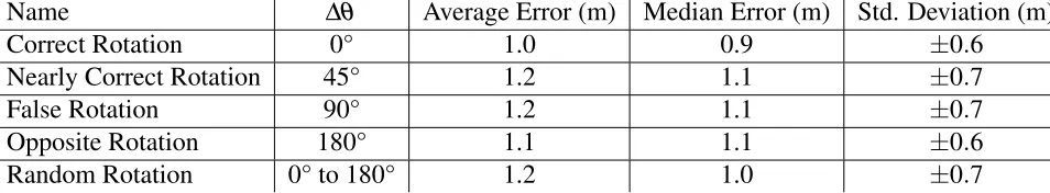
Name ∆θ Average Error (m) Median Error (m) Std. Deviation (m)

Correct Rotation 0° 1.0 0.9 ±0.6

Nearly Correct Rotation 45° 1.2 1.1 ±0.7

False Rotation 90° 1.2 1.1 ±0.7

Opposite Rotation 180° 1.1 1.1 ±0.6

Random Rotation 0° to 180° 1.2 1.0 ±0.7

Table 4.1: A baseline of distance errors for LANDMARC using various grid rotations relative to the target tag’s true rotation.

tag for use in our experiments. Table 4.1 shows distance error metrics for various ∆θ

values.

We can see in Table 4.1 that as the angle difference increases towards 90° we gain

larger average errors in our location estimation, as well as higher standard deviation. At

180°, the tag’s back is again facing the antenna, and provides less error than 90°. Since

a passive RFID tag reflects outwardly from both of its faces, this result is expected. We

can see that it has higher error than 0°, which is most likely because our RFID tag has

a cardboard backing that helps secure it to the apparatus used to conduct the experiment.

This cardboard absorbs some of the radio signal, thereby weakening the received signal in

that direction and reducing our accuracy.

4.4 Related Works

Some localisation algorithms utilize various sensors in addition to RFID tags to

gather more information about the possible orientation of the tag. These sensors could

be accelerometers, temperature, camera, magnetic field, motion, etc. Although not RFID,

[10] aims to utilize most devices found on smart phones to improve localisation accuracies

of the device. Likewise, [11] utilizes an accelerometer to localize an active RFID tag

with-out any reference tags by broadcasting the accelerometer data to a system that can calculate

the next position of the tag based on acceleration values. These values could help

deter-mine additional information such as tag orientation. Since our system will utilize low-cost,

off-the-shelf passive RFID tags that have no dedicated battery, and no on-board CPU, such

(44)

Lim, Choi, and Lee [17] describe how a grid of passive tags, similar to LANDMARC,

can be used to estimate the position, and even orientation of a mobile robot. This is done

by using a moving antenna stationed on the bottom of the mobile robot, and continuously

estimating the movement of the robot using position, and orientation data. We recognize the

benefits of moving an antenna to find additional information about the system, but desire a

(45)

Chapter 5 Solving Rotation Challenge via Rotation

Dimension Reduction

5.1 Solution Inspiration

Our research started with the various factors associated with RFID RSSI for

locali-sation, as well as the established algorithms discussed in recent papers on the topic. Each

algorithm that we found while performing a survey of the state of the art of RFID

localisa-tion attempted to solve some or most of the challenges that we have discussed in Seclocalisa-tion

3.4. A common problem in all of the algorithms is that they are not specifically designed

to solve tag rotations, nor did the papers discuss how tag rotations affect the results of their

systems. We then made it our focus to determine how to utilize tag rotations to improve

most existing RFID localisation systems.

LANDMARC is one of the algorithms that solves almost all challenges that we had

categorized, except for the tag’s rotation. By applying our algorithm for reducing the effects

of rotation on localisation to LANDMARC, we allow LANDMARC to solve all challenges

that we have discussed. By sacrificing set-up time, multiple grids were created at various

rotations that could allow us to augment the LANDMARC algorithm to include the rotation

dimension empirically. By having a hands-on application, we were able to test many ideas

to see how they performed with LANDMARC. The ideas we derived were:

(46)

1. To predict the rotation, then utilize the same rotation training data when performing

comparisons. We constructed various algorithms for trying to predict the rotation of

a tag, with only some being successful.

2. To aggregate each position’s rotations, thereby creating a single grid of training data.

This approach by far had the most success.

By seeing how LANDMARC was affected by the strategies, we will be able to

ab-stract the solution to other localisation algorithms that utilize a comparison between new

samples and training samples. We determined that Rotation Dimension Reduction via

Av-erage was a great solution for not only adding rotations to a localisation system, but to

also reduce the effects of reflection and line-of-sight obstruction by utilizing more

infor-mation about the environment via rotations of the training samples. We discovered why

comparing an average of rotations outperforms a 100% perfect rotation prediction system,

and consider how it might be applied to other localisation techniques.

5.2 LANDMARC Rotation Extension Algorithm

Our algorithm extends the LANDMARC algorithm [23] by including the ability to

rotate a tag by any Y-axis degree, and gain more accurate results than the original

sys-tem due to the additional training information required by our algorithm. We utilize extra

rotational training data to perform a more accurate version of the k-nearest neighbours

algorithm usually used by LANDMARC. We do this by decreasing the error margin of a

comparison between a newly read tag, and each training tag. This is performed by reducing

the total variance of the comparison by aggregating the rotations of tag training data.

The first step of our algorithm requires that one trains multiple grids in addition to

the single grid required by LANDMARC. Each grid should be trained at incremental steps

θ, such that the total amount of grids created will be Number o f Grids= 360◦

θ . For our empirical results, we have chosen a resolution ofθ =45◦, and postulate that lower

Passive RFID Rotation Dimension Reduction via Aggregation

Scholarship at UWindsor

Scholarship at UWindsor

Passive RFID Rotation Dimension Reduction via Aggregation

Passive RFID Rotation Dimension Reduction via Aggregation

Aggregation

Passive RFID Rotation Dimension Reduction via

Aggregation

Eric Matthews

Abstract

Contents

Acronyms

List of Figures

Chapter 1

Thesis Layout

The Problem

Importance

Previous Solutions

New Solution

Thesis Statement

Originality

Non-Triviality

Proof

Explanation

Other Discplinary Uses

Conclusion

Chapter 2

Radio Frequency Identification

2.1

Object Identification via Unique Code

2.2

Active and Passive Tags

2.3

RFID Antennas and Polarization

2.4

Antenna Gain and Path Loss

∑

2.5

Passive RFID Backscatter

RFID Localisation

3.1

Object Tracking and Localisation

3.2

Applications

3.3

Localisation Algorithm Categories

3.3.1

Localisation by Moving Antennas

3.3.2

Localisation by Machine Learning (ML)

3.3.3

Localisation by Geometric Estimation

3.4

Localisation Challenges

3.4.1

Challenge 1: Environmental Changes

3.4.2

Challenge 2: Reflections

3.4.3

Challenge 3: Tag Rotations

Influence of Rotations on LANDMARC

4.1

LANDMARC and Extensions

4.2

LANDMARC Rotation Challenge

4.3

LANDMARC Rotation Baselines

4.4

Related Works

Chapter 5

Solving Rotation Challenge via Rotation

Dimension Reduction

5.1

Solution Inspiration

5.2

LANDMARC Rotation Extension Algorithm