Scalable adaptive collaborative filtering

Scalable

adaptive

collaborative

filtering

João Nuno Vinagre Marques da Silva

Tese de Doutoramento apresentada à

Faculdade de Ciências da Universidade do Porto

Informática

2016

PhD

Ph

Scalable

adaptive

collaborative

filtering

João Nuno Vinagre Marques da Silva

MAPi - Doutoramento em Informática

Universidade do Porto - Faculdade de Ciências Departamento de Ciência de Computadores LIAAD - INESC TEC

2016

Orientador

Alípio Mário Guedes Jorge Professor Associado

Faculdade de Ciências da Universidade do Porto LIAAD - INESC TEC

Coorientador

João Portela da Gama Professor Associado

Faculdade de Economia da Universidade do Porto

Acknowledgements

First and foremost, I would like to thank my supervisor, Prof. Al´ıpio Jorge and my co-supervisor, Prof. Jo˜ao Gama. Their commitment to my success in the development of this thesis was notorious, both by the enriching discussions we had and by their constant encouragement to pursue my goals. Also, of course, for their friendship.

During more than four years, I had the chance to share my work experiences with col-leagues from the Computer Science Department in the Faculty of Sciences of the University of Porto and LIAAD-INESC TEC. I particularly thank Amir Nabizadeh with whom I shared the workplace and had the most fun discussions about recommender systems. I also thank everyone at LIAAD for their friendship and the great work environment. A huge thanks to Joana Dumas, for always being there for me (and everyone else) with the traveling, scheduling, form filling, and all the bureaucracy.

I was fortunate to have met Pawel Matuszyk, with whom I have collaborated, together with our supervisors. We became friends. Like me, he is a big enthusiast of recommender systems and we share many thoughts on science, technology, R&D and other related subjects. Our discussions on recommender systems were tremendously helpful for my work and, I hope, for his work too.

My work could not have been conducted without the financial support by FCT - Fundac¸˜ao para a Ciˆencia e Tecnologia, the portuguese foundation for science and technology, with the research grant SFRH / BD / 77573 / 2011. I am also grateful for the funding from European Regional Development Fund (ERDF) through FCT in projects “SIBILA” (NORTE - 07 - 0124 - FEDER - 000059) and “PEST” (FCOMP - 01 - 0124 - FEDER - 037281) and for the European Commission’s support of project MAESTRA (Grant no. ICT - 2013 - 612944). Part of the work on this thesis is also integrated in Project “TEC4Growth” (NORTE 01 -0145 - FEDER - 000020), financed by the North Portugal Regional Operational Programme (NORTE 2020), under the PORTUGAL 2020 Partnership Agreement, and through the European Regional Development Fund (ERDF).

Finally, I would like to thank my family. I thank my parents for supporting me unconditionally and for being proud of me. My greatest thank is for the two most important and beloved women in my life, my girlfriend Eliana and my daughter Miriam. For putting up with me and for giving meaning to everything I do. This work would not have taken place, and this thesis would not exist without them. Obrigado!

Abstract

Online communities are growing. Human beings, both as individuals and as organizations, benefit from the availability of easily accessible information. This contributes to the dissem-ination of information, knowledge and culture. However, it also makes information filtering harder, due to the overwhelming amount of content from a huge variety of sources. Search engines play a fundamental role in helping users to find relevant content. However, they have the limitation that users need to know what they are looking for, and how to describe it in a query string.

Recommender systems complement search engines by recommending relevant content to users, even if they are not aware of the existence of that very content. This is especially helpful when choosing from a large collection of items, such as in music streaming ser-vices, TV on demand providers, book stores or travel agencies. Collaborative Filtering is a powerful technique to compute personalized recommendations. It uses preference history from a large community of users to infer personalized preferences for individual users. In most real-world systems, recommender algorithms work in an environment where data is continuously being generated. In this thesis, we address the problem of learning rec-ommendation models from such continuous flows of user-generated data – data streams. We focus specifically on streams of positive-only data, that consists exclusively of user-item interactions indicating positive preferences. We propose algorithms that are able to deal with the streaming data environment, as well as learn accurate recommendation models from positive-only user feedback data.

We compare our algorithms with both classic and state-of-the-art alternatives. To do this, we use a highly informative evaluation methodology – prequential evaluation – specifically designed for algorithms that learn from data streams. Our results show that our proposals are able to outperform the alternatives in terms of both predictive ability and running time.

Resumo

As comunidades online est˜ao a crescer. O ser humano, individualmente ou em organiza-c¸˜oes, beneficia da disponibilidade de informac¸˜ao facilmente acess´ıvel. Isto contribui para a disseminac¸˜ao de informac¸˜ao, conhecimento e cultura. No entanto, dificulta a filtragem da informac¸˜ao, dada a esmagadora quantidade de conte´udos e a enorme variedade de fontes. Os motores de pesquisa desempenham um papel fundamental, ajudando utilizadores a encontrar conte´udos relevantes. No entanto, exigem que eles saibam exatamente o que procuram, e como descrevˆe-lo textualmente.

Os sistemas de recomendac¸˜ao complementam os motores de pesquisa encontrando con-te´udos relevantes para os utilizadores, mesmo que estes n˜ao tenham conhecimento pr´evio da sua existˆencia. Isto ´e especialmente ´util na escolha entre uma grande colec¸˜ao de itens, como acontece em servic¸os destreamingde m´usica,TV on demand, livrarias ou agˆencias de viagem. A Filtragem Colaborativa ´e uma t´ecnica poderosa que produz recomendac¸˜oes personalizadas. Usa o hist´orico de preferˆencias de uma grande comunidade de utilizadores para inferir preferˆencias para utilizadores individuais.

Na maioria dos sistemas reais, os algoritmos de recomendac¸˜ao funcionam num ambiente em que os dados s˜ao continuamente gerados. Nesta tese, abordamos o problema da aprendizagem de modelos de recomendac¸˜ao a partir desses fluxos cont´ınuos de dados. Focamos especificamente em dados s´o-positivos, que consistem em interac¸˜oes utilzador--item que indicam exclusivamente preferˆencias positivas. Propomos algoritmos capazes de lidar com o ambiente the fluxo cont´ınuo de dados, bem como aprender modelos de recomendac¸˜ao com alta precis˜ao a partir de dados s´o-positivos.

Comparamos os nossos algoritmos com alternativas do estado-da-arte e cl´assicas. Para fazˆe-lo, usamos uma metodologia de avaliac¸˜ao altamente informativa – avaliac¸˜ao prequen-cial – especificamente desenhada para algoritmos que aprendem a partir de fluxos de dados. Os resultados obtidos mostram que as nossas propostas s˜ao capazes de superar as alternativas em termos de capacidade preditiva e tempo de operac¸˜ao.

Contents

2.2 Content-based filtering . . . 30

2.3 Collaborative filtering . . . 32

2.3.1 Types of feedback . . . 32

2.3.2 Neighborhood-based algorithms . . . 34 9

2.3.2.3 Neighborhood-based CF for positive-only data . . . 37

2.3.3 Matrix factorization methods . . . 37

2.3.3.1 Stochastic gradient descent . . . 39

2.3.4 Matrix factorization for positive-only data . . . 41

2.3.5 Learning to rank - BPRMF . . . 42

2.3.6 Other methods . . . 45

2.4 Hybrid recommenders . . . 45

2.5 Context-aware collaborative filtering . . . 46

2.6 Time-aware and time dependent CF . . . 46

2.6.1 Approaching the time dimension . . . 47

2.6.2 Time-aware algorithms: time as context . . . 48

2.6.2.1 Time-aware factorization models . . . 48

2.6.2.2 Time-aware neighborhood models . . . 50

2.6.2.3 Other time-aware contributions . . . 50

2.6.3 Time-dependent algorithms: time as sequence . . . 51

2.6.3.1 Time-dependent neighborhood models . . . 51

2.6.3.2 Time-dependent factorization models . . . 53

2.6.3.3 Short-/Long-term preference modeling . . . 55

2.6.3.4 Data-stream algorithms . . . 55

2.6.3.5 Data pre-processing . . . 56

2.6.3.6 Euclidean embedding . . . 56

2.6.4 Algorithms both time-aware and time-dependent . . . 56

2.6.5 Discussion . . . 57

2.7 Summary . . . 58 10

3 Collaborative Filtering with streaming data 59

3.1 Data streams . . . 59

3.2 Incremental neighborhood methods . . . 61

3.2.1 Incremental user-based CF . . . 61

3.2.2 Incremental user-based CF for positive-only feedback . . . 62

3.2.3 Incremental item-based collaborative filtering . . . 64

3.2.4 Limitations of neighborhood-based incremental CF . . . 64

3.3 Incremental matrix factorization . . . 64

3.3.1 Incremental BRISMF . . . 65

3.3.2 Incremental learn-to-rank . . . 66

3.3.2.1 Incremental BPRMF . . . 67

3.4 Forgetting . . . 67

3.4.1 Forgetting for neighborhood-based incremental CF . . . 69

3.4.2 Forgetting with factorization-based incremental CF . . . 69

3.5 Summary . . . 71

4 Stream-based recommendations with negative feedback 73 4.1 Proposed algorithm - ISGD . . . 74

4.1.1 Stream-based bagging . . . 75

4.2 Negative preference imputation . . . 79

4.2.1 Weighting methods . . . 79

4.2.2 Sampling methods . . . 81

4.2.3 Graphical models . . . 82

4.3 Recency-based negative feedback . . . 82

4.3.1 Recency-based algorithm . . . 83

4.3.2 Rate-based algorithm . . . 86

4.4 Summary . . . 89 11

5.2 Prequential evaluation . . . 94

5.2.1 Limitations . . . 95

5.3 Online evaluation . . . 96

5.4 Experimental process details . . . 96

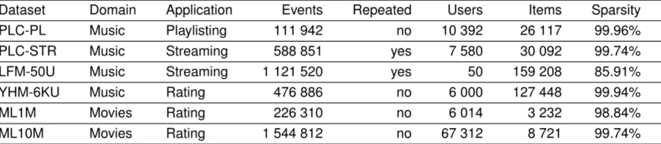
5.4.1 Datasets . . . 96 5.4.2 Experimental process . . . 98 5.4.3 Metrics . . . 98 5.4.4 Statistical significance . . . 99 5.4.5 Parameter optimization . . . 100 5.4.6 Presentation of results . . . 100

5.4.7 Software and hardware . . . 101

5.5 Comparing incremental and batch learning . . . 101

5.5.1 Results . . . 102

5.5.2 Discussion . . . 102

5.6 ISGD with bagging . . . 105

5.6.1 Discussion . . . 105

5.7 ISGD with recency-based negative feedback . . . 108

5.7.1 Impact in processing time . . . 108

5.7.2 Rate-based negative feedback . . . 113

5.7.3 Discussion . . . 115

5.8 Comparison with other algorithms . . . 116

5.8.1 Optimal parameters . . . 116

5.8.2 Results . . . 117

5.8.3 Discussion . . . 120 12

5.9 Summary . . . 124

6 Conclusions 127 6.1 The impact of time . . . 127

6.2 The data stream approach . . . 128

6.3 Learning from positive-only ratings . . . 129

6.4 Evaluating stream-based recommenders . . . 129

6.5 Limitations . . . 130

6.6 Future work . . . 130

A List of Abbreviations 133 B Additional plots 135 B.1 ISGD with bagging . . . 135

B.2 ISGD with recency-based negative feedback . . . 139

B.3 Comparison with other algorithms . . . 145

List of Tables

5.1 Dataset description . . . 97

5.2 Comparison between BSGD and ISGD . . . 103

5.3 ISGD with bagging . . . 106

5.4 Aggregated results of RAISGD . . . 109

5.5 Differences of update times between RAISGD and ISGD . . . 112

5.6 Optimal parameter settings for ISGD, RAISGD, BPRMF and WBPRMF . . . . 117

5.7 Overall results with RAISGD, ISGD, BPRMF, WBPRMF and UKNN . . . 119

List of Figures

2.1 Example of feedback matrices. On the left, a typical numerical ratings matrix.

On the right a positive-only ratings matrix. . . 33

2.2 Matrix factorization: R=ABT. . . 38

2.3 CANDECOMP/PARAFAC tensor factorization model. . . 49

4.1 Evolution of Recal@10 of ISGD through the incremental learning and predic-tion process, illustrating the degradapredic-tion of ISGD over time. . . 83

4.2 Recency-based negative feedback imputation . . . 85

4.3 Evolution of Recal@10 of ISGD and RAISGD through the incremental learn-ing and prediction process, illustratlearn-ing the degradation of ISGD over time. . . 86

5.1 Prequential evaluation . . . 94

5.2 Prequential evaluation of Recall@10 with BSGD and ISGD . . . 104

5.3 Prequential evaluation of Recall@10 with ISGD using bagging . . . 107

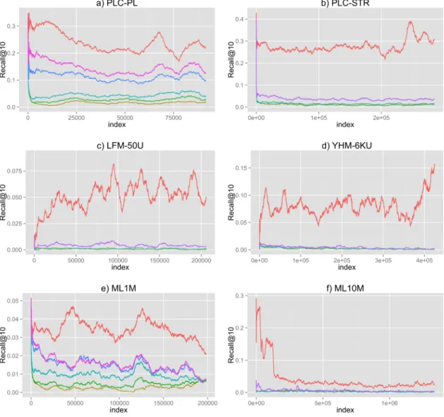
5.4 Prequential evaluation of Recall@10 with 6 datasets for RAISGD . . . 110

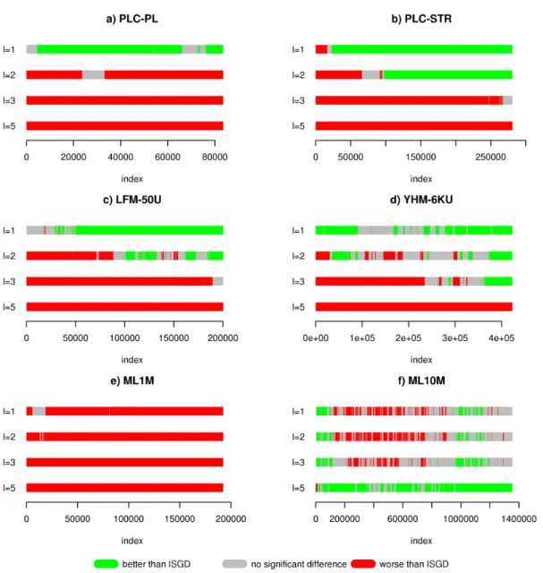
5.5 Signed McNemar pairwise test between Recall@10 obtained by RAISGD and ISGD . . . 111

5.6 Online update times in milliseconds of RAISGD with 6 datasets . . . 113

5.7 Prequential evaluation of Recall@10 with 6 datasets for RAISGD . . . 114

5.8 Signed McNemar pairwise test between Recall@10 obtained by RAISGD and RAISGD-RB . . . 115

5.9 Prequential evaluation of Recall@10 with 6 datasets . . . 120 17

5.11 Online update times in milliseconds with 6 datasets . . . 122

B.1 Prequential evaluation of Recall@1 with ISGD using bagging . . . 136

B.2 Prequential evaluation of Recall@5 with ISGD using bagging . . . 137

B.3 Prequential evaluation of Recall@20 with ISGD using bagging . . . 138

B.4 Prequential evaluation of Recall@1 with 6 datasets for RAISGD . . . 139

B.5 Prequential evaluation of Recall@5 with 6 datasets for RAISGD . . . 140

B.6 Prequential evaluation of Recall@20 with 6 datasets for RAISGD . . . 141

B.7 Signed McNemar pairwise test between Recall@1 obtained by RAISGD and ISGD . . . 142

B.8 Signed McNemar pairwise test between Recall@5 obtained by RAISGD and ISGD . . . 143

B.9 Signed McNemar pairwise test between Recall@20 obtained by RAISGD and ISGD . . . 144

B.10 Prequential evaluation of Recall@1 with 6 datasets . . . 145

B.11 Prequential evaluation of Recall@5 with 6 datasets . . . 146

B.12 Prequential evaluation of Recall@20 with 6 datasets . . . 147

B.13 McNemar pairwise tests between RAISGD and other algorithms, relative to the Recall@1 metric . . . 148

B.14 McNemar pairwise tests between RAISGD and other algorithms, relative to the Recall@5 metric . . . 149

B.15 McNemar pairwise tests between RAISGD and other algorithms, relative to the Recall@20 metric . . . 150

List of Algorithms

2.1 BSGD - Batch SGD . . . 40

2.2 BSGD - Batch SGD for positive-only data . . . 41

2.3 BPRMF - Bayesian Personalized Ranking Matrix Factorization . . . 44

3.1 UKNN - User-based incremental algorithm (training) . . . 63

3.2 UKNN - User-based incremental algorithm (recommendation) . . . 63

3.3 Incremental user feature updates . . . 65

3.4 BPRMF - incremental version . . . 68

4.1 ISGD-SI - Incremental SGD for positive-only ratings with single iteration . . . . 75

4.2 ISGD - Incremental SGD for positive-only ratings, with multiple iterations . . . 76

4.3 BaggedISGD - Bagging version of ISGD (training) . . . 78

4.4 RAISGD: Recency-Adjusted ISGD . . . 84

4.5 RAISGD-RB: Recency-Adjusted ISGD (Rate-Based) . . . 88

Chapter 1

Introduction

The amount of content available on the internet, as well as in enterprise and governmental information systems is overwhelming. It is not possible for human beings to browse through all the content available on large online commerce catalogs, text-based and multimedia databases and social networks, without some kind of automated filtering. This has long ago motivated the development of information filtering algorithms. The most obvious example are implemented in search engines such as Yahoo!, Google or Bing. These algorithms typically allow users to conveniently filter content using simple text queries. For example, if a user wants to find a strawberry pie recipe, she would naturally query her favorite search engine with the text “strawberry pie recipe”. The algorithm then matches the query to a

huge collection of indexed content and displays the results as a list, usually ordered by relevance.

The importance of information filtering is nowadays evident. For instance, in December 2014, 3 of the top 5 most active internet domain names belong to general purpose search engines [Alexa Website Rankings, 2015; Similarweb Website Rankings, 2015], according to Alexa1 _{and SimilarWeb}2_{, two popular worldwide traffic rankings. However search engines}

are designed for on-demand retrieval, which means that users have to know what they are looking for. This is not always possible or even desirable. When a user wishes to find content that is unknown to her, she obviously would not know how to formulate a text query to describe it. Typical examples of this are the discovery of music, movies, books, TV shows, touristic destinations, news and e-learning content, although there is no fundamental restriction on the type of content to be discovered. For instance, when a user wishes to find new movies to watch or music to listen to, the problem is how to find novel content that matches the user’s preferences. This is one example of a typical recommendation task, and systems that aim to solve this and other similar problems are

1_{http://www.alexa.com} 2_{http://www.similarweb.com}

known asrecommender systems.

Over the past two decades, an increasing number of researchers has focused on Recom-mender Systems. Collaborative Filtering (CF) is one extensively studied recommendation method. It consists of using historical information about all users in a system to perform personalized recommendations to specific users. CF has been successfully used in a large number of applications, such as e-commerce websites [Linden et al., 2003] and other on-line communities in a series of domains [Resnick et al., 1994; Hill et al., 1995; Shardanand and Maes, 1995]. Competitions like the Netflix prize [Bennett et al., 2007], the KDD-Cup 2011 [Dror et al., 2012], the Million Song Challenge [McFee et al., 2012], the successive ACM RecSys Conferences, Workshops and Challenges, as well as the increased demand from both the academic community and the industry, have motivated many notable contributions in the field.

1.1 Motivation

Real-world online systems continuously generate data. However, most algorithms and techniques available in the literature on recommender systems fail to acknowledge this. Instead, they are designed to learn recommendation models from large static datasets containing user feedback collected from the system in which they operate. The dataset is then analyzed and a model is inferred. This model then remains essentially unchanged until another large chunk of data is available to retrain a new model. This approach raises two problems. The first problem arises from the system’s unawareness of the continuous activity of users in the system for arbitrary amounts of time. The exact same model is used to perform recommendations for minutes, hours, days, weeks, months or years. As user preferences change over time and users and items enter and leave the system, the model becomes increasingly inaccurate. The second problem is computational. As the amount of collected data increases, the necessary computational resources to store it and process it also increase. Processing ever-growing data in batch eventually leads to scalability issues, even if the algorithm complexity grows linearly with the size of data. Systems either need to be scaled up – which can be expensive – or data needs to be reduced – which can mean throwing away potentially valuable information.

Many researchers have focused on both of these problems, but mostly independently of each other. Time related issues in recommender systems have been investigated in many contributions in the field [Campos et al., 2014; Vinagre et al., 2015b]. Regarding the com-putational problem, algorithms are becoming increasingly efficient in learning from large amounts of data. Additionally, distributed models are becoming more mature, flexible and widespread, enabling the use of recommendation algorithms and techniques that otherwise

1.1. MOTIVATION 23 would not be applicable [Low et al., 2012; Owen et al., 2011]. However, even this paradigm still has the fundamental limitation that the volume of data eventually becomes too high to be stored and processed.

One possible alternative is to consider data stream approaches [Domingos and Hulten, 2000] and apply them to the recommendation problem [Vinagre et al., 2014b; Matuszyk and Spiliopoulou, 2014]. Algorithms that learn from online data streams acknowledge two important aspects. First, the concepts that algorithms try to capture are typically non-stationary – they vary with time. In this sense, these concepts constitute a moving target. Second, data streams are potentially unbounded, while computational resources are limited and/or expensive. Ideally, algorithms should be able to operate independently from the number of examples. By approaching user feedback data that recommenders learn from as a data stream, these two aspects are inherently acknowledged. Algorithms that deal with data streams have been successfully used in many fields of application, such as medical systems, energy systems and computer networks [de Andrade Silva et al., 2013; Aggarwal, 2014]. However, recommender systems do not typically approach data as a stream. In this thesis, we approach recommendation as a data stream problem, simply by ac-knowledging that the process that generates user feedback data – used in the training of recommendation models – is continuous and never stopping. We use algorithms that are able to learn from such streams of data by maintaining incremental models, and evaluate them using well studied protocols designed for streaming environments.

In this thesis we focus exclusively on positive-only user feedback streams. These are streams that only contain positive interactions between users and items, and provide no information on non-positive – neutral and negative – opinions. The main motivation to focus our research on positive-only data is availability. Practically any system that involves users and items already has a source of positive-only feedback. The examples are countless: web logs, music streaming history, shopping habits, social network sharing and “liking”, news reading, watched movies or series, point-of-interest check-ins, to name just a few of them. These typically consist of continuous flows of user-item pairs, that indicate a positive preference of a user for an item. Unlike recommender systems that deal with ratings – like a numeric scale, like 1 to 5 stars – systems that deal with positive-only data face the problem of not having information about negative preferences – the items that users do not like. This hardens the task of finding good items to recommend, because it is not easy to distinguish between items users do not like – not good for recommendation –, and items that users simply do not know – the ideal recommendation candidates [Vinagre et al., 2015a; Pan et al., 2008]. Additionally, algorithms that learn from positive-only data are also usable with ratings data, which makes them universally applicable to user-item interaction datasets. Given our general problem setting, which is to learn recommendation models from

positive-only user feedback streams, we also need to use an evaluation methodology that is ap-plicable to this setting. Traditional methods designed for batch-learning algorithms are not suitable for algorithms that learn from data streams [Gama et al., 2013; Vinagre et al., 2014a], so we need to use a framework that allows the continuous evaluation of such algorithms. Evaluation methods and protocols for data stream algorithms are available in the literature, however we are not aware of any research that uses those methods in recommender systems. The evaluation of recommendation algorithms is typically done in offline, controlled environments. When compared to recommender systems running online with real users, in such a laboratory environment, researchers have more independence and freedom, in the sense that they do not depend so much on third parties. By avoiding the constraints of real-world applications, it is possible to focus research on very specific prob-lems, without having to worry about external factors. However, as a natural consequence, problems caused by the very constraints that are circumvented in offline research are very rarely addressed. To evaluate our work, we use an evaluation methodology specifically designed for algorithms that learn from data streams that is designed to be used in online environments.

1.2 Research questions

The motivation above leads to the following four research questions (RQ).

RQ1 Do phenomena related with time have a significant impact on recommendation? If so, is the existing knowledge in the field of recommendation sufficient to approach time related problems? These phenomena encompass user preference changes over time – which can be fast and abrupt or slow and gradual –, the contin-uous incoming and outgoing of new users and items that naturally happen in online systems, seasonal effects. To answer this question, we study the state-of-the-art of usage-based recommendation techniques that deal with time, explicitly or implicitly. We address this question in Chapter 2.

RQ2 Are batch learning approaches adequate and sufficient to deal with all the chal-lenges of real world recommender systems? Could the techniques and algo-rithms for data streams be used to improve the accuracy and/or scalability of recommender systems? To answer this, we argue that the ever increasing amount of data necessarily leads to both accuracy loss and heavy constraints on performing batch learning, given that computational resources are always limited. Based on the available knowledge on algorithms that learn from data streams, we investigate novel methods that are able to incrementally maintain recommendation models, as well as techniques to exploit the time dimension in the context of recommendation.

1.3. CONTRIBUTIONS 25 We propose an incremental matrix factorization algorithm based on state-of-the-art methods, designed to deal with incoming data streams of user feedback. We assess the benefits of using such techniques under the typical constraints of data stream environments. This question is addressed in Chapters 3 and 4.

RQ3 Considering the known problems of dealing with positive-only data for rec-ommendation, can we devise a scheme that mitigates those problems that is compatible with the streaming approach? Can we exploit the time dimension to do this? Given that we use positive-only data, we need to deal with the effect of not having negative feedback to help the algorithms in distinguishing between good and bad recommendations. We propose a temporal scheme based that uses the recency of occurrence of items to select negative examples that are artificially introduced in the stream of feedback data. We address this in Chapter 4.

RQ4 Are traditional evaluation protocols suitable for recommender systems running on dynamic real-world environments? If not, how de we evaluate recommen-dation algorithms in such environments? In order to evaluate algorithms, we need an evaluation methodology that enables fair and accurate comparison between algorithms that maintain dynamic models. We use an evaluation framework based on well studied evaluation methods for data stream mining. We use this framework to assess the accuracy and speed of our proposed algorithms. We cover this in Chapter 5.

1.3 Contributions

In this thesis we provide four contributions.

• We survey the state-of-the-art on recommendation systems, with particular focus on

the ones that deal with temporal effects. Based on this study, we find that exploiting time is generally beneficial in recommender systems, and identify the most important related challenges.

• We propose a matrix factorization algorithm that learns a recommendation model in

fast incremental steps. This enables the model to continuously learn from single data points as they arrive in a stream of user feedback.

• We show that diversity techniques are beneficial in recommendation models that learn

from data streams. We propose the use of online bagging – bootsrap aggregating – to improve the accuracy of our incremental matrix factorization algorithm.

• We introduce two recency based mechanisms to (a) solve the problem of learning exclusively from positive examples and (b) exploit the recency of occurrence of items, taking advantage of the time dimension.

• We devise an evaluation methodology specifically for recommender systems that

learn from data streams. Typical evaluation protocols used with batch algorithms are simply not applicable in an environment where data keeps flowing in. We use a well known evaluation framework for data streams – prequential evaluation – to evaluate recommendation algorithms in a streaming environment. We also present new forms of visualization of results, as well as the visualization of statistical signifi-cance of the difference between algorithms. These visualizations show the evolution of performance of algorithms over time, as they process incoming data.

1.4 Organization

After this chapter, this thesis is divided in five more chapters.

In Chapter 2, we discuss the concepts that constitute the building blocks in our research, focusing on RQ1. We identify the tasks of recommender systems, and provide a general view on the classes of algorithms that can be used to accomplish those tasks, with special focus on the ones that are directly useful for the understanding of the remainder of the thesis. We also provide an overview on algorithms that exploit time information to improve recommendation.

Chapter 3 focuses on RQ2, specifically on recommendation algorithms that are capable of learning from data streams of usage data. We start by describing the specific proper-ties data streams, and the requirements of algorithms that learn from such flows of data. We analyze several algorithms and techniques that are suitable for recommendation with streaming data.

To answer the second part of RQ2, we propose, in Chapter 4, an incremental matrix factor-ization algorithm (Algorithm 4.2 - ISGD), along with BaggedISGD, an ensemble version of ISGD that uses bagging, and also RAISGD and RAISGD-RB, two versions of ISGD that use recency-based technique to tackle the challenges of learning from positive-only (specifically addressing RQ3).

In Chapter 5 we evaluate our proposed algorithms, essentially addressing RQ4. We start by describing the prequential evaluation process, as used in data streams. Then we use that methodology to evaluate our proposals, in four stages. First, we measure the benefits of using ISGD by comparing it with its batch-learning version. Second, we evaluate the use of bagging with ISGD. Third, we evaluate the recency-based negative feedback imputation

1.5. LIST OF PUBLICATIONS 27 schemes presented in Chapter 4, by comparing how several amounts of negative feedback perform with respect to the original ISGD algorithm (without negative feedback imputation). Fourth, we compare ISGD, with and without negative feedback imputation, with a classic and well known neighborhood-based algorithm and two versions of a state-of-the-art algo-rithm.

Finally, we draw conclusions in Chapter 6, by presenting the core of our findings, the limitations of our proposals, and future lines of work that can complete or complement this thesis.

We also add three Appendixes. We list abbreviations used in the text of the thesis in Appendix A. To avoid the excessive proliferation of graphics in Chapter 5, we move to Appendix B several auxiliary plots. These plots are referenced in the text where they may become relevant.

1.5 List of publications

The following papers have been published (by order of appearance):

• [Vinagre et al., 2014b] Jo˜ao Vinagre, Al´ıpio M´ario Jorge, and Jo˜ao Gama. Fast

incremental matrix factorization for recommendation with positive-only feedback. In Proceedings of the 22nd International Conference on User Modeling, Adaptation, and Personalization (UMAP 2014), Aalborg, Denmark, July 7-11, 2014. Volume 8538 of Lecture Notes in Computer Science, pages 459–470. Springer, 2014.

• [F´elix et al., 2014] Catarina F´elix, Carlos Soares, Al´ıpio M´ario Jorge, and Jo˜ao

Vina-gre. Monitoring recommender systems: A business intelligence approach. In Pro-ceedings of the 14th International Conference on Computational Science and Its Applications (ICCSA 2014), Guimar˜aes, Portugal, June 30 - July 3,2014. Volume 8584 of Lecture Notes in Computer Science, pages 277–288. Springer, 2014.

• [Vinagre et al., 2014a] Jo˜ao Vinagre, Al´ıpio M´ario Jorge, and Jo˜ao Gama.Evaluation

of recommender systems in streaming environments. In Proceedings of the Workshop on Recommender Systems Evaluation: Dimensions and Design (REDD 2014) in conjunction with the 8th ACM Conference on Recommender Systems (RecSys 2014), Foster City, CA, USA, October 10, 2014.

• [Vinagre et al., 2015a] Jo˜ao Vinagre, Al´ıpio M´ario Jorge, and Jo˜ao Gama. Collab-orative filtering with recency-based negative feedback. In Proceedings of the 30th ACM SIGAPP Symposium on Applied Computing (SAC 2015), April 13-17, 2015, Salamanca, Spain. Pages 963–965. ACM, 2015.

• [Matuszyk et al., 2015] Pawel Matuszyk, Jo˜ao Vinagre, Myra Spiliopoulou, Al´ıpio M´ario Jorge, and Jo˜ao Gama.Forgetting methods for incremental matrix factorization in recommender systems. In Proceedings of the 30th ACM SIGAPP Symposium on Applied Computing (SAC 2015), April 13-17, 2015, Salamanca, Spain. Pages 947–953. ACM, 2015.

• [Vinagre et al., 2015b] Jo˜ao Vinagre, Al´ıpio M´ario Jorge, and Jo˜ao Gama. An overview

on the exploitation of time in collaborative filtering. Wiley Interdisciplinary Reviews: Data Mining and Knowledge Discovery, 5(5):195–215, 2015.

In [Vinagre et al., 2014b], we present two contributions directly related to this thesis. First, we propose the incremental matrix factorization algorithm for positive-only data described in Chapter 4 (Algorithm 4.1). We also introduce the evaluation methodology described with detail in Chapter 5. In [Vinagre et al., 2014a], we focus specifically on the benefits of this evaluation methodology, namely by using significance tests over time.

In [Vinagre et al., 2015a], we propose a recency-based scheme that improves the per-formance of algorithms that deal with positive-only data. This contribution is also directly related to this thesis, and is described in Section 4.3.

A survey on the exploitation of the time dimension is available in [Vinagre et al., 2015b]. This is a contribution that focuses on algorithms that are able to take advantage of the time dimension to improve recommendation. This contribution is also available in Section 2.6. Finally we had two collaboration works. In [Matuszyk et al., 2015], we study forgetting strategies for recommendation with incremental matrix factorization algorithms. This work is closely related to our past work in [Vinagre and Jorge, 2012], and is a parallel line of work of this thesis. We describe our major findings in Section 3.4. In [F´elix et al., 2014], we study the performance monitoring of recommender systems from a business intelligence perspective. Our findings show that business intelligence tools are effective in monitoring the performance of recommendation models over time.

Chapter 2

Recommender Systems

This thesis focuses on specific issues of recommender systems. However, to describe these issues, some introductory background and context are necessary. This chapter pro-vides a general introduction to recommender systems, focusing on the concepts, definitions and techniques that constitute the framework for the remainder of the thesis. In Section 2.6, we also provide an overview on the emergent techniques that deal with time-related aspects, such as seasonality or preference changes over time.

2.1 Tasks of a recommender system

Recommender systems are typically designed for online communities encompassing a large number of users – typically human beings – that browse through a large number of items in the system. Items can be movies, music, books, touristic attractions, restaurants or any other kind of product or content of interest. Users and items are the two central entities in all recommendation problems.

Even though the idea behind all recommender systems is essentially the same – recom-mend items to users –, there is quite a variety of end-user tasks in which recomrecom-mender systems can assist. Herlocker et al. identify the following tasks in [Herlocker et al., 2004]:

• Annotation in context: this consists on the annotation of items with a value that

indicates how much will the item be liked by the user. The recommender system only needs to predict this value. The most obvious example is predicting the rating – e.g. in a one to 5 star scale – a user would give to any particular item, and displaying that to the user. This is also known asrating estimationorrating prediction.

• Find good items: many users use recommender systems to find a set of items that

consists of the best items for them, i.e. the items the user is most likely to prefer. Recommender systems can achieve this either by sorting the top-N items according to a score – e.g. their predicted rating –, or by directly approaching the recommendation task as a ranking problem. This task is often referred to astop-N recommendation.

• Find all good items: here the task is similar toFind good itemstask, with the

require-ment of not missing any good recommendation.

• Recommend sequence: when items are consumed sequentially, the order by which

they are recommended is crucial. Automatic music playlist generation is one good example of this task. The main objective is to find a good sequenceof items, rather than a set – most likely ordered by relevance – that the user can access in an arbitrary order.

• Just browsing: some users may just find interesting or entertaining to browse through

a provider’s catalog, even if there is no imminent interest of consumption and/or purchase. Users here are more interested in the navigation functionality and style provided by recommender systems.

• Find credible recommender: some end-users browse through several recommender

systems just testing how well they match their actual tastes, until they find one that is satisfactory. This is a common task of new users. Of course, while testing, users can only evaluate recommendations of items that they already know, so there is a natural bias towards perhaps less valuable recommendations.

All of the above tasks have implications in the problem formulation and evaluation methodol-ogy and metrics. For example, the metrics used to evaluaterating estimationare naturally different from the ones used for evaluating the recommendation of item sequences. The measurement of the overall quality of a recommender system is highly dependent on the task for which the recommender is designed.

As Herlocker et al. state in [Herlocker et al., 2004], the vast majority of research focuses on either one of the two first tasks. In this thesis we focus on top-N recommendation – Find good items.

2.2 Content-based filtering

Content-based filtering provides recommendations by analyzing user profiles or history [Pazzani and Billsus, 2007], and matching the obtained information to the items’ content. For example, in a system that recommends news, if the available information about a user

2.2. CONTENT-BASED FILTERING 31 indicates a preference for technology and arts, then news with relevant content about these fields of interest will be recommended. This approach requires that some information about the user is available. This information can be obtained in two ways [Pazzani and Billsus, 1997; Mooney and Roy, 2000]:

• explicitly: user profiles are built based on information, such as demographic

informa-tion or preferences explicitly specified, provided by the users themselves;

• implicitly: user activity history, such as purchased items on an e-commerce website,

is analyzed and recommendations are made accordingly.

Content-based filtering works when information about users is available and when it is possible to extract information from the items content that we can relate to user profiles or history. The first problem arises from the need to obtain information about users, since it is not possible to make reliable recommendations if user information is not available or incomplete [Adomavicius and Tuzhilin, 2005].

Another problem consists of the limitations of content analysis [Shardanand and Maes, 1995; Balabanovic, 1997]. It is a fact that computers have limited abilities when it comes to interpret and recognize content, especially non-textual content. While text content is relatively easy to analyze and extract information from, analyzing multimedia content – for example, audio, video or images – can potentially become an extremely complex task. For instance, recommending action movies to a user known to like them would require that the system was able to accurately detect genre in video files. The most obvious and used way to work around this problem is to add meta-data to items, such as text attributes [Pazzani and Billsus, 2007]. This way it is possible to relate items to user preferences. In many systems, however, the large number of items can make it prohibitive to add attributes to items [Shardanand and Maes, 1995].

A system based on user profiles may also suffer from super-specialization [Balabanovic, 1997]. When a user profile determines some preference, only items that match that pref-erence are recommended. In many cases, this can be the desired behavior, but in other cases it can be a limitation. For example, a user with a preference for italian restaurants would never receive a recommendation for other type of restaurants, no matter its popularity or quality. On the other hand, recommending all italian restaurants is probably not a useful recommendation.

Although not abundant in recent literature – when compared with collaborative filtering –, recent advances in multimedia content analysis, such as image and speech recognition, have provided new tools and techniques for the research in content-base recommendation. Techniques based on Neural Networks combined with optimization based learning, fre-quently referred to as Deep Learning [Bengio, 2009; Arel et al., 2010; Schmidhuber, 2015],

together with the advances in parallel computation have allowed the large scale analysis of multimedia content. This research is, however, out of the scope of this thesis.

2.3 Collaborative filtering

As mentioned in the beginning of this chapter, many on-line virtual communities consist of a large number of users that browse through items in the system. Items can be movies, music, books, touristic attractions, restaurants or any other kind of product of interest. In such systems, users are frequently allowed to give their personal opinion about items, by rating that item either explicitly – e.g. using a “like” button or a 5 star rating scale – or implicitly – e.g. number of times a user listens to a music track, or whether a user has bought some item or not. Suppose a system has n users and m items. By collecting

feedback from users, it is possible to build a user-item feedback matrixRn⇥mcontaining all ratings given by users to items. TypicallyRis a very sparse matrix – users usually only rate

a very small proportion of the items in the system. By exploiting the preferences of similar users, Collaborative Filtering (CF) algorithms try to make predictions about individual user preferences. CF algorithms achieve this by learning or training a predictive model with the available usage data: the matrix R. This model can then be used to predict the user

preferences that are missing in R. The best way to train this recommendation model is

dependent on the type of feedback being analyzed.

2.3.1 Types of feedback

One important distinction, which determines the choice or development of an algorithm, is the one between the two possible types of user feedback data:

• Numeric ratings feedback: typically composed of triples in the form(u, i, r), consisting

of the rating valuer being given by useruto itemi;

• Positive-only or unary feedback: a set of pairs in the form(u, i), representing a positive

interaction between useruand itemi.

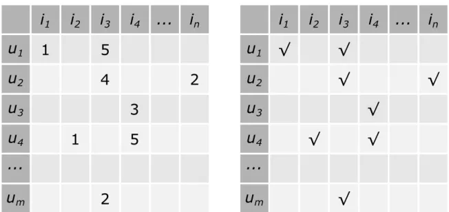
The content of the user-item matrix is naturally different for the two above types of feedback. Figure 2.1 illustrates user-item matrices for both ratings and positive-only data. When numeric ratings are available, the main task typically consists of predicting missing values in the user-item matrix. This is a natural formulation when numeric ratings are available, and the problem is naturally seen as a rating predictiontask. However, some systems employ positive-only ratings. These systems are quite common – e.g. like/favoritebuttons, music

2.3. COLLABORATIVE FILTERING 33

Figure 2.1: Example of feedback matrices. On the left, a typical numerical ratings matrix. On the right a positive-only ratings matrix.

streaming, shopping carts, news reading. In these cases, the matrixR is a boolean value

matrix, wheretruevalues indicate a positive user preference, andf alse– typically the vast

majority – may indicate one of two things: the user either does not like or does not know the item. In systems with positive-only user feedback, the task is to predict truevalues in R,

which is more closely related to classification problems. This type of feedback is also known in the literature as binary ratings or implicit feedback. We adopt the term positive-only, since the term binary may suggest the existence of both positive and negative feedback and the termimplicitmay not be accurate – for instance, clicking alikebutton can hardly be considered an implicit preference. Recommendation using positive-only feedback is also known in the literature asone-class collaborative filtering [Pan et al., 2008].

Considering our focus on thetop-N recommendation task, the type of feedback being used has important implications. For example, when using numeric ratings, a recommendation list can be easily produced by sorting items by descending predicted rating. This, however, is not so trivial when using positive-only data. Generally, we either need to predict some kind of preference level for items – in order to sort them for each user – or to directly approach the task as a learning to rank problem [Liu, 2009].

Most state-of-the-art CF algorithms are based on either neighborhood methods or matrix factorization methods. Fundamentally, these differ on the strategy used to process data in the ratings matrix.

2.3.2 Neighborhood-based algorithms

Neighborhood-based CF algorithms essentially compute user or item neighborhoods using similarity measures such as the cosine or Pearson correlation [Sarwar et al., 2001]. If the rows of R represent users and the columns correspond to items, similarity between

two users u and v is obtained using the rows corresponding to those users, Ru and Rv. Similarity between two items iandj can be obtained between the columns corresponding

to those itemsRi andRj. Recommendations are computed by searching and aggregating through user or item neighborhoods. The main advantages of neighborhood methods are their simplicity and ease of implementation, as well as the trivial explainability of recom-mendations – user and item similarities are intuitive concepts. The main downside of neighborhood-based methods is the lack of scalability, since that both time and space complexity grow simultaneously with both the number of users and the number of items in the system.

2.3.2.1 User-based CF

User-based CF exploits similarities between users to form user neighborhoods. Given two users u and v, the similarity between them is given by a measure, typically the Pearson

Correlation and the Cosine.

Cosine measure For two usersuandv, the cosine measure takes the rows of the ratings

matrixRu andRv as vectors in a space with dimension equal to the number of items rated byuandv: sim(u, v) = cos(Ru, Rv) = Ru·Rv ||Ru||⇥||Rv|| = P i2IuvRuiRvi qP i2IuR 2 ui qP i2IvR 2 vi (2.1)

where Ru ·Rv represents the dot product between Ru and Rv,Iu and Iv are the sets of items rated byuandvrespectively andIuv=Iu\Iv is the set of items rated by both users

uandv.

A common problem with the cosine is that different users may use the rating scale differently. For example, in a system with a rating scale of integers from 1 to 5, one user can interpret the value 3 as a positive rating, while another user can see it as negative rating. This means that different preference levels can be expressed using the same value. Conversely, equal preference levels may result in different ratings.

2.3. COLLABORATIVE FILTERING 35 Pearson Correlation For usersuandv, the Pearson Correlation is given by:

sim(u, v) = P i2Iuv(Rui R¯u)(Rvi R¯v) qP i2Iuv(Rui R¯u) 2qP i2Iuv(Rvi R¯v) 2 (2.2)

where _R¯_{u and R}¯_{v are the average ratings given by users u and v, respectively. These}

averages have a normalizing effect on ratings given by different users, minimizing the scale interpretation problem.

Rating prediction To compute a rating prediction _Rˆ_{ui given by the user u to item i, an}

aggregating function is used that combines the ratings given toiby the subsetKu ✓U of thekusers most similar tou– the optimal value ofkcan be obtained using cross-validation.

Two examples of this function are [Adomavicius and Tuzhilin, 2005; Breese et al., 1998]:

ˆ Rui= P v2Kusim(u, v)Rvi P v2Kusim(u, v) (2.3) ˆ Rui= ¯Ru+ P v2K_Pusim(u, v)(Rvi R¯v) v2Kusim(u, v) (2.4) Equation (2.3) performs a weighted average, in which weights are given by the similarities betweenuandv. Equation (2.4) incorporates the average ratings given byuandvin order

to minimize differences in how users use the rating scale.

2.3.2.2 Item-based CF

Similarity between items can also be explored to provide recommendations [Sarwar et al., 2001; Linden et al., 2003]. The main motivation for the use of item-based algorithms is that many systems have a larger number of users than items. In such systems the dimension of the similarity matrix is significantly reduced using item-based CF. As in user-based algorithms, Cosine and Pearson Correlation can be used as item-user-based similarity measures:

Cosine measure LetUi andUj be the set of users that rated itemsiand j respectively, andUij =Ui\Ujthe set of users that co-ratedbothitemsiandj. The similarity betweeni andj is given by the cosine of the angle formed by vectorsRi andRj, whose coordinates are the ratings given by all users to each of the items:

sim(i, j) = cos(Ri, Rj) = Ri·Rj ||Ri||⇥||Rj|| = P u2UijRuiRuj qP u2UiR 2 ui qP u2UjR 2 uj (2.5)

As in the user-based case, the cosine for item-based similarity suffers from the scale interpretation problem – different users have different interpretations of the rating scale. For item-based cosine similarity the adjusted cosine [Sarwar et al., 2001] can be used instead:

sim(u, v) = P u2Uij(Rui ¯ Ru) (Ruj R¯u) qP u2Ui(Rui R¯u) 2qP u2Uj(Ruj R¯u) 2 (2.6)

In the above equation, the average rating_R¯_{ugiven by useruis used to minimize the effect}

of different interpretations of the rating scale.

Pearson Correlation The Pearson Correlation can also be used in item-based algorithms as a measure of similarity between two itemsiandj. It is given by:

sim(i, j) = P u2Uij(Rui R¯i)(Ruj R¯j) qP u2Uij(Rui ¯ Ri)2qP_u2Uij(Ruj R¯j)2 (2.7)

where_R¯_iandR¯_{j are the average ratings given toiandj, respectively.}

Rating prediction According to [Sarwar et al., 2001], the prediction of the rating givenuto

itemiis obtained like this: letKibe the set of items most similar toi. Then, an aggregating function such as one of the two below is used:

ˆ Rui= P j2Kisim(i, j)Ruj P j2Kisim(i, j) (2.8) ˆ Rui= ¯Ri+ P j2Kisim(i, j)(Ruj ¯ Rj) P j2Kisim(i, j) (2.9) Equation (2.8) is the weighted average of the ratings given by u to the items similar toi.

The similarity values sim(i, j) are the weighting factors. In (2.9) the average rating given

to i and j are used to eliminate eventual biases on how those items are rated. Like in

the user-based case, the optimal number of nearest-neighbors Ki is typically obtained via cross-validation.

2.3. COLLABORATIVE FILTERING 37 2.3.2.3 Neighborhood-based CF for positive-only data

The methods in Section 2.3.2 are designed to work with numerical ratings. However, our focus in this thesis is on positive-only data. Neighborhood-based CF for positive-only data can actually be approached as a special case of neighborhood-based CF for ratings, by simply consideringRui = 1for all observed(u, i) user-item pairs andRui = 0for all other cells in the feedback matrix R. Both notation and implementation can be simplified with

this. With positive-only data, the rating scale interpretation problem does not apply. The most practical similarity measure is then the cosine, given by (2.1). In the user-based case, it can be simplified to:

sim(u, v) = cos(Ru, Rv) = P i2IuvRuiRvi qP i2IuR 2 ui qP i2IvR 2 vi = p|(Iu\Iv)| |Iu|⇥ p |Iv| (2.10) whereIu andIv the set of items that are observed withuandj, respectively.

In the item-based case, the simplification is analogous:

sim(i, j) = cos(Ri, Rj) = P u2UijRuiRuj qP u2UiR 2 ui qP u2UjR 2 uj = p|(Ui\Uj)| |Ui|⇥p|Uj| (2.11)

In (2.11),Ui andUj are the set of users that are observed withiandj, respectively. The cosine formulation in (2.10) and (2.11) for positive-only ratings allows the calculation of user-user or item-item similarities using simple user occurrence and co-occurrence counts. A useruis said to co-occur with userv for every itemithey both occur with. Similarly, an

itemiis said to co-occur with itemjevery time they both occur with a user u. A prediction

for user u and itemican be made using one of (2.3) or (2.4), in the user-based case, or

(2.8), in the item-based case. One important notion is that the value of_Rˆ_{uiis not a rating,}

but rather a score between 0 and 1, by which a list of candidate items for recommendation can be sorted in descending order for every user.

2.3.3 Matrix factorization methods

The most studied alternative to neighborhood-based CF is Matrix Factorization (MF). So far, MF methods have proved to be generally superior to neighborhood methods in large scale problems, in terms of both predictive ability and run-time complexity [Shi et al., 2014]. Matrix Factorization for CF was initially inspired by Latent Semantic Indexing [Deerwester et al., 1990], a popular technique to index large collections of text documents, used in the

field of information retrieval. LSI performs the Singular Value Decomposition (SVD) of large document-term matrices. In a CF problem, the same technique can be used in the user-item matrix, uncovering a latent feature space that is common to both users and user-items. One important feature of SVD is that it provides the ability to make optimal lower rank approximations to the original matrix. One problem with SVD is that classic factorization algorithms, such as Lanczos methods, are not defined for sparse matrices. This issue has been addressed by performing some form of value imputation in the user-item matrix [Billsus and Pazzani, 1998; Sarwar et al., 2000b]. This, however, is a potential source of systematic error, especially taking into account that the user-item matrix in CF problems is typically very sparse.

As an alternative to classic SVD, optimization methods [Bell and Koren, 2007; Funk, 2006; Paterek, 2007; Tak´acs et al., 2009] have been proposed to decompose (very) sparse user-item matrices1_.

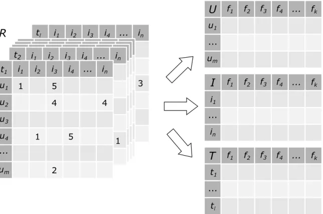
Figure 2.2: Matrix factorization:R =ABT_.

Figure 2.2 illustrates the factorization problem. Supposing we have a user-item matrixRm⇥n withmusers andnitems, the algorithm decomposesRin two full factor matricesAm⇥kand

Bn⇥k that, similarly to SVD, cover a commonk-dimensional latent feature space, such that

R is approximated by Rˆ =ABT_{. MatrixA spans the user space, whileB spans the item} space. The k latent features describe users and items in a common space. Given this

formulation, the predicted rating by useruto itemiis given by a simple dot product: ˆ

Rui=Au·Bi (2.12)

The number of latent features k is a user given parameter that controls the model size.

Individual latent features can represent simple and easy to understand concepts, as well 1_{In some of the literature, these methods are often referred to as SVD, despite being formally different} methods.

2.3. COLLABORATIVE FILTERING 39 as complex high level concepts and their combinations. For instance, in a movie rating dataset, one latent feature may encode a specific genre – e.g. action, comedy, horror – while another may encode complex features such as Oscar winning movies from the late seventies. The semantics of latent features is not known a priori, however a good algorithm should be able to extract the most important ones for the given data. A good exploratory analysis is done in [Tak´acs et al., 2009], where the authors are able to identify the implicit encoding of genre on latent features.

2.3.3.1 Stochastic gradient descent

The model consists ofAandB, so the training task consists of estimatingAandBsuch as

their product approximates R as accurately as possible. This is done by minimizing error

on the known ratings. Training is performed by minimizing theL2-regularized squared error

for known values inR and the corresponding predicted ratings:

min

A.,B.

X

(u,i)2D

(Rui Au·Bi)2+ u||Au||2+ i||Bi||2 (2.13) In the above equation,Dis the set of user-item pairs for which ratings are known and is

a parameter that controls the amount of regularization. The regularization terms ||Au||2 and i||Bi||2 are used to avoid overfitting. These terms penalize parameters with high magnitudes, that typically lead to overly complex models with low generalization power. For the sake of simplicity, we use = u = i, which results in a single regularization term (||Au||2 +||Bi||2). The rank of the factor matrices A and B – the number of latent features k – is a user-defined hyperparameter that can be used to control the trade-off

between model size and information loss. The most computationally efficient methods to solve this optimization problem are Alternating Least Squares (ALS) [Bell and Koren, 2007] and Stochastic Gradient Descent (SGD) [Funk, 2006]. It has been shown [Funk, 2006; Paterek, 2007] that SGD based optimization generally performs better than ALS when using very large and sparse datasets – which is typically the case in recommender systems –, both in terms of model accuracy and run time performance. In this thesis, we study the simple case of processing data over a single CPU, however some interesting alternatives to simple SGD are available in the literature that are able to take advantage of parallel processing platforms [Gemulla et al., 2011; Yu et al., 2014] and/or Graphical Processing Units [Rodrigues et al., 2015].

Given a training dataset consisting of tuples in the form(u, i, r)– the ratingrof useruto item i–, SGD performs several passes through the dataset, known as iterations or epochs, until

of iterations. At each iteration, SGD sweeps over all known ratings Rui and updates the corresponding rowsAu andBi, correcting them in the opposite direction of the gradient of the error, by a factor of ⌘  1– known as step size or learn rate. The algorithm starts by

initializing matrices A andB with small random numbers – typically following a gaussian2

N(µ, ) with µ = 0 and and small . For each known rating, the corresponding error is

calculated aserrui=Rui Rˆui, and the following update operations are performed:

Au Au+⌘(erruiBi Au)

Bi Bi+⌘(erruiAu Bi)

(2.14)

Algorithm 2.1:BSGD - Batch SGD

Data: a datasetD= (u, i, r)1, . . . ,(u, i, r)n

input :kthe no. of latent features

input :iterthe no. of iterations

input : the regularization factor input :⌘the learn rate

output:Athe user factor matrix

output:B the item factor matrix

1 init 2 foru₂Users(D)do 3 Au Vector(size:k) 4 Au⇠N(0,0.1) 5 fori₂Items(D)do 6 Bi Vector(size:k) 7 Bi⇠N(0,0.1)

8 forcount 1toiterdo

9 D Shuffle(D)

10 for(u, i, r)₂Ddo

11 errui r Au·Bi

12 Au Au+⌘(erruiBi Au)

13 Bi Bi+⌘(erruiAu Bi)

Algorithm 2.1 implements this method. It has first been informally proposed in [Funk, 2006] and many extensions have been proposed ever since [Paterek, 2007; Koren, 2008; Tak´acs et al., 2009; Salakhutdinov and Mnih, 2007]. One obvious advantage of SGD is that complexity grows linearly with the number of known ratings in the training set, actually taking advantage of the high sparsity ofR.

2_{We use}

2.3. COLLABORATIVE FILTERING 41 Other proposed factorization methods include probabilistic Latent Semantic Analysis (pLSA), used in [Hofmann, 2004] and [Takacs et al., 2007], and CF via Principal Component Analy-sis (PCA) [Goldberg et al., 2001].

2.3.4 Matrix factorization for positive-only data

Algorithm 2.1 (BSGD) is designed to work with ratings data. The input of the algorithm is a set of triples in the form(u, i, r), each corresponding to a rating r given by a useru to an

itemi. It is possible to use BSGD with positive-only data by simply assuming thatr= 1for

all cases. This results in Algorithm 2.2.

Algorithm 2.2:BSGD - Batch SGD for positive-only data

Data: a datasetD= (u, i)1, . . . ,(u, i)n

input :kthe no. of latent features

input :iterthe no. of iterations

input : the regularization factor input :⌘the learn rate

output:Athe user factor matrix

output:Bthe item factor matrix

1 init 2 foru2Users(D)do 3 Au Vector(size:k) 4 Au ⇠N(0,0.1) 5 fori2Items(D)do 6 Bi Vector(size:k) 7 Bi⇠N(0,0.1)

8 forcount 1toiterdo

9 D Shuffle(D)

10 for(u, i)2Ddo

11 errui 1 Au·Bi

12 Au Au+⌘(erruiBi Au)

13 Bi Bi+⌘(erruiAu Bi)

The only differences between Algorithms 2.1 and 2.2 are the type of input data and the error calculation. Algorithm 2.2 receives pairs in the form(u, i)and assumesr = 1, causing errui to be calculated as the difference to 1 always. In the end, the predicted “ratings”

ˆ

Rui =Au.Bi will be a value indicating a user’s preference level for an item. This value can be used in a sorting functionf to order a list of items:

fui=|1 Rˆui| (2.15)

Equation (2.15) measures the proximity of a predicted rating to 1. If we look at BSGD, it is evident that what it models is exactly this. Au andBi are always adjusted to minimize the error with respect to 1, so it is natural to assume that the most relevant items for a useru

are the ones that minimize the difference above. Note that since we are not imposing on the model any restrictions to the prediction values, which means that_Rˆ_{uiis not restricted to}

the interval[0,1]. This is why we use the absolute value of the difference in (2.15).

One important limitation of using BSGD with positive-only data is that it could result in trivial models. If we use a model where _Rˆ_{ui = 1 for all (u, i) pairs, the error would always be} errui= 1 Rˆui= 0, and no learning would be performed. This does not happen in practice for two reasons. First, regularization squashes down the values of feature vectors with high magnitude, which in practice forces predictions to always be_Rˆ_{ui<1. Second, we initialize}

the feature vectors with random values close to 0, which forces the model to always begin a learning process. Although regularization and model initialization may help prevent trivial solutions, they do not entirely solve the problem. When learning from large datasets – which is a common scenario in recommender systems – most predictions will tend to accumulate closely together, eventually leading to a model with low discriminative power. One solution is to try to counterbalance the model with negative examples that can be inferred from the positive ones. We discuss this technique in Chapter 4. Another solution is to approach the recommendation problem directly as a learning-to-rank problem.

2.3.5 Learning to rank - BPRMF

If we look at the top-N recommendation problem, we are in fact trying to obtain a list of ranked items. Learning-to-rank algorithms [Liu, 2011] directly model the relative position between items in a list. In [Rendle et al., 2009], Rendle et al. use a Bayesian framework to capture personalized item rankings. Given the set of usersU and the set of itemsI in

a dataset consisting of positive user-item interactions (u, i), the task consists of finding an

optimal item ranking >u for each user – i.e. a personalized ranked set of items. This set follows the three poperties of a total order. For any useru, the personalized rankIu of any itemsi,jandkinI is such that:

• ifi >uj andj >u itheni=j(antisymmetry)

• ifi >uj andj >u ktheni >u k(transitivity)

2.3. COLLABORATIVE FILTERING 43 Instead of scoring items for users, Rendle et al. devise a ranking model, that establishes a personalised rank of items for each user >u, by assuming that all items i observed for that user – the observed pairs (u, i) in the dataset – precede, in >u, all items j that do not occur withuin the dataset. The Bayesian formulation – Bayesian Personalize Ranking

(BPR) – consists of maximizing the posterior probability p(⇥_| >u), where ⇥ represents the parameters of an arbitrary model. This formulation is especially helpful because it is independent of the predictive model. Effectively, BPR is applicable to both neighborhood and factorization models. We will focus on BPR with Matrix Factorization – BPRMF. In this case,⇥ = (A, B), withA andB being the two factor matrices representing user and item

latent features respectively. Learning is performed using triples in the form (u, i, j), that

correspond to the actual observed pair(u, i)with an additional itemjsampled from the set

of items not observed withu. PredictionsRˆuij indicate the relative rank ofiandj, which is expressed by the difference between the dot products:

ˆ

Ruij =Au·Bi Au·Bj (2.16)

This allows the use of conventional matrix factorization, together with SGD to train a ranking model. The update operation for the parameter set⇥in the SGD algorithm is:

⇥ ⇥+⌘( ( ˆRuij)

@

@⇥Rˆuij+ ⇥⇥) (2.17)

where⌘ is the learn rate, is the logistic function (x) = ₁₊e_exx and ⇥ is a set of

regu-larization factors for the parameters. In the matrix factorization algorithm, three parameter vectors are updated at each iteration:

Au Au+⌘( (Au·Bi Au·Bj)(Bi Bj) + uAu)

Bi Bi+⌘( (Au·Bi Au·Bj)Au+ iBi)

Bj Bj +⌘( (Au·Bi Au·Bj)Au+ jBj)

(2.18)

Note that three different regularization factors u, iand j need to be set. Algorithm 2.3 is the complete implementation of BPRMF.

In Algorithm 2.3, k, iter, ⌘ and the three _{u,i,j} are respectively the number of latent

features, the number of iterations, the learn rate and the regularization factors for users, observed items and unobserved items. The SampleFrom typically performs uniform

sam-pling from the set of items that the user has not interacted with. A variant of this algorithm, that is known as Weighted BPRMF – or WBPRMF – performs non-uniform sampling from the same set, by sampling items with probability proportional to their popularity.

Algorithm 2.3:BPRMF - Bayesian Personalized Ranking Matrix Factorization

Data: a datasetD= (u, i)1, . . . ,(u, i)n

input :kthe no. of latent features

input :iterthe no. of iterations

input : u, i and j the regularization factors

input :⌘the learn rate

output:Athe user factor matrix

output:B the item factor matrix

1 init 2 foru₂Users(D)do 3 Au Vector(size:k) 4 Au⇠N(0,0.1) 5 fori₂Items(D)do 6 Bi Vector(size:k) 7 Bi⇠N(0,0.1)

8 forcount 1toiterdo

9 D Shuffle(D) 10 for(u, i)₂Ddo 11 j SampleFrom(_{j_|(u, j)₂/D_}) 12 Au Au+⌘( (Au·Bi Au·Bj)(Bi Bj) + uAu) 13 Bi Bi+⌘( (Au·Bi Au·Bj)Au+ iBi) 14 Bj Bj+⌘( (Au·Bi Au·Bj)Au+ jBj)

2.4. HYBRID RECOMMENDERS 45

2.3.6 Other methods

Although the majority of research on algorithms for recommender systems is focused on either neighborhood or matrix factorization methods, other alternatives have been proposed to solve CF problems. Probabilistic strategies, such as Clustering and Bayesian networks, have been presented in early work [Breese et al., 1998]. Clustering is motivated by the assumption that it is possible to group users in clusters according to their preferences. In [George and Merugu, 2005; Symeonidis et al., 2006; de Castro et al., 2007],co-clustering

– or bi-clustering – simultaneously clusters users and items, with gains in computational performance and without significant accuracy loss. The reasoning behind co-clustering it that it is frequent that users in a cluster prefer specific subsets of items.

Other probabilistic approaches are based on Graph Theory [Aggarwal et al., 1999; Huang et al., 2002, 2004; Fouss et al., 2007; Gori and Pucci, 2007; Tiroshi et al., 2014]. For systems with binary ratings, Association Rules [Sarwar et al., 2000a; Mobasher et al., 2001; Lin et al., 2002] and Markov Chains [Shani et al., 2005; Rendle et al., 2010] have also been proposed.

In [Khoshneshin and Street, 2010], the MF problem is reformulated as an Euclidean em-bedding problem that joins users and items in a common Euclidean space. The model is learned with SGD in a analogous process to MF and Euclidean distances between users and items are directly used to predict ratings.

2.4 Hybrid recommenders

There is no fundamental constraint on combining content-based filtering with collaborative filtering. A third type of recommender systems, known as hybrid recommendation, does exactly that, taking advantage of both collaborative filtering and content-based filtering. Fundamentally, hybrid recommender systems vary in the strategy used to combine rec-ommendation methods from the two worlds, for which there is a considerable variety of approache