Development of a biologically-based controlLed growth and differentIation model for developmental toxicology

Development of a Biologically-Based Controlled Growth and

Differentiation Model for Developmental Toxicology

Shree Y. Whitaker1, Hien T. Tran1 and Christopher J. Portier2 Abstract

The biologically-based dose-response model for developmental toxicology developed by Leroux et al. (1996) is extended. The original model had two basic states; precursor cells and differentiated cells with both states subject to a linear birth-death process. In this paper, a mathematical model, which is biologically and statistically based, is developed with a highly controlled birth and death process for precursor cells. This model limits the number of replications allowed in the development of a tissue or organ and more closely reflects the presence of a true stem cell population. The mathematical formulation of the Leroux et al.

(1996) model was derived from a partial differential equation for the generating function that limits further expansion into more realistic models of mammalian development. The same formulae for the probability of a defect (a system of ordinary differential equations) can be derived through the Kolmogorov forward equations due to the nature of this Markov process. This modified approach is easily amenable to the expansion of more complicated models of the developmental process such as the one presented here. Comparisons between the Leroux et al. (1996) model and the controlled growth and differentiation (CGD) model as developed in this paper are also discussed.

KEY WORDS: teratology; multistate process; cellular kinetics 1. Introduction

There has been considerable research into the mechanistic basis through which environmental exposures can initiate and promote disease processes. Much of this research has focused on the molecular and biochemical basis describing the interaction of chemical and physical agents with healthy tissue. Most environmental health risk assessments are focused on the rates of morbidity and mortality in human populations following an environmental exposure. The linkage between basic biology and disease incidence in environmental health is best described using a tool which is focused on the incidence of disease and which can fully utilize the emerging science [1,2]. Disease incidence is generally described by counting events (e.g. disease prevalence in a population) or by early, functional failure of an entire organ system (e.g. disease incidence per year). Data endpoints such as these require a different mathematical treatment than the mathematical treatment applied to absorption, distribution and metabolism data endpoints [3]. While the mechanistic basis for

1

Center for Research in Scientific Computation, Department of Mathematics, Box 8205, North Carolina State University, Raleigh, North Carolina 27695-8205.

2

understanding environmentally induced disease has progressed rapidly, biologically-based mechanistic models of morbidity and mortality lag far behind. This gap in development is partially due to the difficulties in the mathematical treatment of these endpoints and partially due to gaps in our understanding of how they occur.

The scientific database for a mechanistic understanding of toxic effects following chemical exposure is probably greatest for the area of carcinogenesis. Several researchers have published work in the area of multistage models for carcinogenesis. The Armitage-Doll model [4] is considered the grandfather of the multistage cancer models. This model has been widely used for the analysis of epidemiological data and for cancer risk assessment. From the statistical point of view, this model provides a broad class of hazard functions for the analysis of data. Armitage and Doll [5] extended this model to use a deterministic linear birth-death process on the intermediate state in a two-stage model. Several other researchers

[6-23]

have also contributed significant progress to this field. The models developed use biologically based information and basic stochastic processes (generally interconnected birth-death processes with immigration and emigration) to reproduce the behavior of cells as they progress through the stages of cancer. Cancer is viewed as a multi-step process in which cells move from a controlled and systematic state of growth into a state of uncontrollable and chaotic growth [24, 25]. The basic assumption – that cancer is a disease of single cells rather than entire organ systems - on which these models were predicated, makes the mathematical modeling of carcinogenesis feasible.

To model a disease process with as much precision as possible, it is imperative to first understand and create a solid foundation for the basic developmental process of a tissue or organ. The linkage is critical in that many of the early markers for carcinogenesis relate back to genes and proteins expressed predominantly during development and cellular replication [26, 27]. Several authors have attempted to create models for the analysis of data from developmental toxicity. Much of this effort has focused on the creation of statistical likelihoods for handling the nested variance observed from developmental toxicology studies or for the longitudinal nature of the data [28-35]. Others have developed statistical models for the probability of a defect focusing on the role of some other form of toxicity (such as maternal toxicity) in the forms of the equations. Leroux et al. [36] developed the first biologically-based, stochastic model of developmental toxicity based on an interconnected birth-death process and using the first and second moments for the number of cells in a second stage of the model as an indicator of the probability of toxicity. The general view of development as modeled by Leroux et al. [36] is a straightforward approach. However, their use of an uncontrolled, linear birth-death process for cellular growth is both biologically unreasonable (for small numbers of cells) and mathematically uncontrollable allowing for no clear numerical constraints on the size of the resulting organ.

et al. [36] model. We will show that the same linear first-order system of ordinary differential equations describing the expectations, squared expectations and the expected cross product of cells in a two-stage model of developmental toxicology can be derived using, alternatively, the Kolmogorov forward equations. This model is then extended in Section 2.2 to allow greater emphasis on the control of growth and differentiation (CGD). We emphasize that the model proposed by Leroux et al. [36] is not a sub-model of the CGD model since a linear birth process is not assumed. Finally, in Section 3, a comparison between the Leroux et al. [36] model and the CGD model is made on the prediction of the effects of methylmercury on brain development in rats and Section 4 contains our concluding remarks.

2. Materials and Methods

Development consists of a series of states during which cells first replicate, then differentiate with some loss of cells and then separate into groups of cells for which a similar function is needed. This cycle is repeated numerous times; some organs and organ systems complete development early while others continue to develop even after birth of the mammal. During the developmental process of a tissue or organ, a cell eventually moves from an uncommitted state to a committed state. This simple characterization of development implies that the rates that drive the formation of a mammal can be classified into one of three categories: birth, death and transformation. This crude, cellular level approach to development can not fully accommodate the subtle biochemical and molecular events, such as expression of key growth factors and hormones, which are really governing overall development, but serves as a phenomenological description of the cellular growth of an organ. These rates (birth, death and transformation) are likely to be functions of these subtler biochemical and hormonal signals.

2.1 The Leroux et al.[36] Model

Equation Section 1

In this section, we will review the mathematical model developed by Leroux et al. [36] for the developmental process for a particular tissue or organ. More specifically, we will show that the same mathematical model, which is a system of ordinary differential equations describing the expectations, squared expectations and expected cross product of cells, can also be derived using the Kolmogorov forward equations. This modified approach is easily amenable to the expansion of more complicated models of the developmental process including the development of a biologically-based controlled growth and differentiation model for developmental toxicology (see Section 2.2).

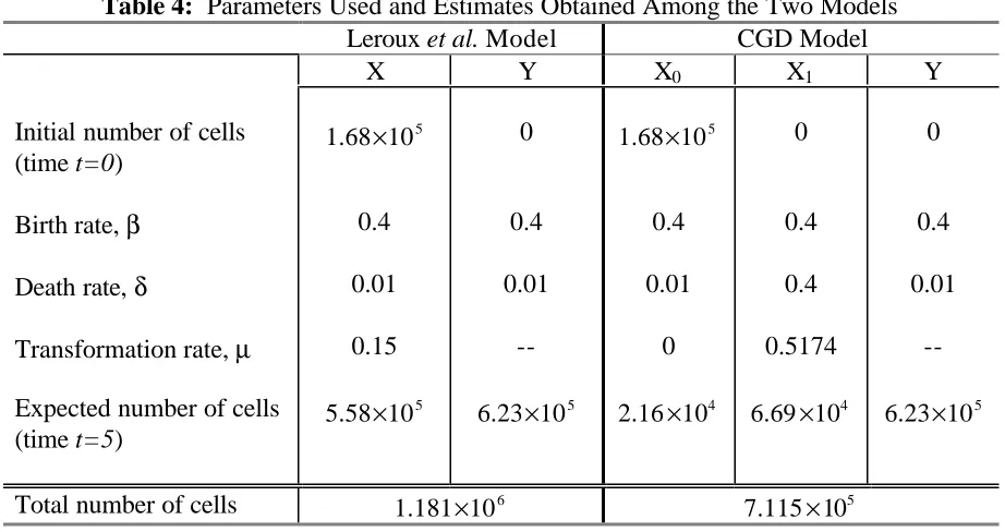
A schematic diagram of the Leroux et al. model is shown in Figure 1. In this model, the basic developmental process is divided into two main subpopulations. Type- X cells represent cells before commitment to differentiation whereas type-Y cells represent cells that have undergone a transformation and are committed to a phenotype. In addition, the following specific assumptions were made for the mathematical development of the model:

(ii) the probability of more than one event in a single cell in any small time interval ∆t

is proportional to o(∆t);

(iii) transformation is an irreversible process;

(iv) a cell in a particular population can only replicate to produce cells of the same population; and

(v) a malformation results when the number of committed (Y t( )) cells is less than a critical number (Y_c) at a specified time, t_c (i.e., ( )Y t_c <Y_c).

The type- Xcell has the option to replicate, die or transform while the type-Y cell may either replicate or die. It is noted that the result of a cell replicating is two daughter cells that are a part of the original population (i.e., the daughter cells are members of the same population as the parent cell). The result of a cell dying is either removal of the cell from the population of properly functioning cells or actual death of a cell. A transformation is the product of a type-X cell moving from the population of uncommitted cells to the population of cells committed to differentiation.

The developmental rates are denoted by β₁( )t (birth rate in X population), δ₁( )t (death rate in X population), β₂( )t (birth rate in Y population), δ₂( )t (death rate in Y population) and µ( )t (transformation rate from X population to Y population). The meaning of the rate

1( )t

β , for example, is that for the time interval [ , ) t t+ ∆t where ∆tis small, the probability of replication for a type- X cell is β₁( )t ∆ + ∆t o( t) where

0

( ) lim 0.

t

o t

t

∆ → ∆∆ = (1.1)

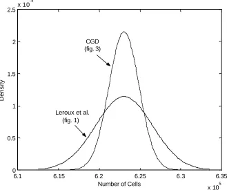
Table 1: Single Cell Event Probabilities in time [ ,t t + ∆t) for the Leroux et al.[36]Model

Event t t+ ∆t Single cell transition probability

X birth x-1,y x,y

0 0

1( )t tPx,y,0( -1, , )x y t

β ∆

X death x+1,y x,y

0 0

1( )t tPx,y,0(x 1, , )y t

δ ∆ +

Y birth x,y-1 x,y

0 0

2( )t tPx,y ,0( ,x y-1, )t

β ∆

Y death x,y+1 x,y

0 0

2( )t tPx,y,0( ,x y 1, )t

δ ∆ +

transformation x+1,y-1 x,y

0,0,0

( )t tPx y (x 1,y-1, )t

µ ∆ +

no change x,y x,y

0 0

1 1

2 2 , ,0

{1- ( ) - ( ) - ( )

( ) ( ) } x y ( , , )

t t t t t t t t t t P x y t

β δ µ

β δ

∆ ∆ ∆

− ∆ − ∆

Since only certain events, which are summarized in Table 1, can occur in a small time interval ∆t, the transition probability

0, 0,0 x y

P is given by

0 0 0 0 0 0

0 0

0 0 0 0

, ,0 1 , ,0 1 , ,0

, ,0

2 , ,0 2 , ,0

1 1

( , , ) ( 1) ( ) ( 1, , ) ( 1) ( ) ( 1, , ) ( 1) ( ) ( 1, 1, )

( 1) ( ) ( , 1, ) ( 1) ( ) ( , 1, )

[1 ( ) ( ) ( )

x y x y x y

x y

x y x y

P x y t t x t tP x y t x t tP x y t

x t tP x y t

y t tP x y t y t tP x y t

x t t x t t x t t y

β δ µ β δ β δ µ + ∆ = − ∆ − + + ∆ + + + ∆ + − + − ∆ − + + ∆ +

+ − ∆ − ∆ − ∆ − β2( )t ∆ −t yδ2( )t ∆t P] x₀,y₀,0( , , ).x y t

(1.3)

We recall that for discrete random variables X and Y, the moment generating function for a time interval of length ∆t given the initial values x0 and y0 is given by

0 0

0 0 , ,0

[ ( ) ( ) | (0) , (0) ] ( , , ).

y

k p k p

x y x

E X t+ ∆t Y t+ ∆t X = x Y = y =

∑

∑

0 0

1 0

0 0

(0) , (0) ] (0) , (0) ]

[ ( ) ( ) |X x Y y [ ( ) |X x Y y

E X t+ ∆t Y t+ ∆t = = = E X t+ ∆t = = (1.5)

0, 0,0( , , )

y

x y x

xP x y t t

=

∑

∑

0 0 0 0

0 0

0 0 0 0

1 , ,0 1 , ,0

, ,0

2 , ,0 2 , ,0

1 1 2

[ ( 1) ( ) ( 1, , ) ( 1, , ) ( 1, 1, )

( , 1, ) ( , 1, ) [1 ( ) ( ) ( ) ( )

( 1) ( ) ( 1) ( )

( 1) ( ) ( 1) ( )

y

x y x y

x

x y

x y x y

x x t tP x y t x y t

x y t

x y t x y t

x x t t x t t x t t y t t

x x t tP

x x t tP

x y t tP x y t tP

β β δ µ β δ µ β δ − ∆ − + + + + − + − + + + − ∆ − ∆ − ∆ − ∆ = + ∆ + ∆ − ∆ + ∆

∑

∑

2( ) ] x y, ,0( , , ).

yδ t t P x y t

− ∆

(1.7)

The first term in equation (1.7) can be simplified by rescaling the summation indices as follows:

0 0 0 0

1 , ,0 1 , ,0

( 1) ( ) ( 1, , ) ( 1) ( ) ( , , )

y y

x y x y

x x

x x β t tP x y t x xβ t tP x y t

′

′ ′ ′

− ∆ − = + ∆

∑

∑

∑

∑

0 0 0 0

1 1

2

, ,0 , ,0

( ) ( , , ) ( ) ( , , )

y y

x y x y

x x

x β t tP x y t xβ t tP x y t

′ ′

′ ′ ′ ′

=

∑

∑

∑

∑

2

1 1

[ ( ) ] ( ) [ ( )] ( ) ,

E X t β t t E X t β t t

= ∆ + ∆ (1.10)

where we used 2

[ ( )]

E X t to denote 2

0 0

[ ( ) | (0) , (0) ]

E X t X = x Y = y . Proceeding in a similar manner for the remaining terms in equation (1.7) leads to

{

}

[ ( )] ( ) ( ) ( ) 1 [ ( )].

Subtracting E X t[ ( )] from both sides of equation (1.11) and then dividing both sides by ∆t

yields

{

}

[ ( )] [ ( )]

( ) ( ) ( ) [ ()],

E X t t E X t

t t t E X t

t β δ µ

+ ∆ − _{= − −}

∆ (1.12)

which, in the limit as ∆tgoes to zero, gives

{

}

[ ( )] ( ) ( ) ( ) [ ( )].

d

E X t t t t E X t

dt = β −δ −µ (1.13)

Analogously, the expected value for the random variable Y can be derived along with the second moments ( 2

0 0

[ ( ) | (0) , (0) ]

E X t X = x Y = y and 2

0 0

[ ( ) | (0) , (0) ]

E Y t X = x Y =y ) and the correlation (E X t Y t[ ( ) ( ) | (0)X =x Y₀, (0)= y₀]). The system of ordinary differential equations describing the means, variances and covariances for the number of cells in states

X and Y at any time t is given by

{

}

[ ( )] ( ) ( ) ( ) [ ( )]

d

E X t t t t E X t

dt = β −δ −µ (1.14)

{

}

[ ( )] ( ) ( ) [ ( ) ] ( ) [ ( )]

d

E Y t t t E Y t t E X t

dt = β −δ +µ (1.15)

{

}

{

}

2 2

1 1

1 1

[ ( ) ] 2 ( ) ( ) ( ) [ ( )] ( ) ( ) ( ) [ ( ) ]

d

E X t t t t E X t

dt

t t t E X t

β δ µ

β δ µ

= − −

+ + +

(1.16)

{

}

{

}

2 2

2 2 2 2

[ ( ) ] 2 ( ) ( ) [ ( )] ( ) ( ) [ ( )] ( ) [ ( )] 2 ( ) [ ( ) ( )]

d

E Y t t t E Y t t t E Y t

dt

t E X t t E X t Y t

β δ β δ

µ µ

= − + +

+ +

(1.17)

{

}

2

[ ( ) ( )] ( ) ( ) ( ) ( ) ( ) [ ( ) ( ) ] ( ) [ ( )] ( ) [ ()].

d

E X t Y t t t t t t E X t Y t

dt

t E X t t E X t

β δ β δ µ

µ µ

= − + − −

− +

(1.18)

The above mathematical model is identical to the one derived by Leroux et al. [36] from considering a partial differential equation for the generating function for X t( ) and Y t( ). In the case of constant rates, the system of differential equations (1.14)-(1.18) is a linear system of ordinary differential equations with constant coefficient of the form

( ) ( )

y tr′ = Ay tr (1.19)

where 2 2

( ) ( [ ( )], [ ( )], [ ( )], [ ( )], [ ( ) ( )])T

1 1

2 2

1 1 1 1

2 2 2 2

1 1 2 2

0 0 0 0

0 0 0

.

0 2( ) 0 0

0 2( ) 2

0 0

A

β δ µ

µ β δ

β δ µ β δ µ

µ β δ β δ µ

µ µ β δ µ β δ

− −

 

 ₋ 

 

 

= + + − −

 _{+ −} 

 

 _{− − − + −} 

 

(1.20)

The exact solution can be written in terms of the eigenvalues and eigenvectors of the matrix

A (see e.g., Braun [37]).

2.2 The Controlled Growth and Differentiation (CGD) Model

Equation Section 2

As already discussed elsewhere in this paper, the mathematical model formulated by Leroux et al. [36], which is based on a linear birth-death process, is both biologically and mathematically unreasonable because it allows no constraint on the size of the resulting organ or tissue. We now describe modifications to the Leroux et al. model that put greater emphasis on the control of growth and differentiation (CGD). More specifically, we consider a multistate developmental process with separate growth phases in the type- X

cells and a linear birth-death process on the type-Y cells. A schematic diagram of the CGD model is illustrated in Figure 2. In this system, there are k+1 specific type-X populations denoted as type- X_i, where i=0,1,2,K,k. Each of the type- X cell populations represents cells prior to commitment to differentiation. Moreover, as a cell moves from one stage, for example from X_i, to the next stage, X_i+1, it matures in the developmental process. By setting µ_i =0, for one or more values of i, we allow for greater control in the type- X cells prior to differentiation. Eventually, the uncommitted cell will undergo a change and join the population of cells already committed to performing a specific function of a tissue or organ. This process by which an uncommitted cell becomes a cell committed to differentiation is termed transformation. Type-Y cells denote the population of cells committed to differentiation.

The developmental rates are again denoted by β_i( )t (birth rate in a X_ipopulation), ( )

i t

δ (death rate in a X_ipopulation), βy( )t (birth rate in the Y population), δy( )t (death rate in the Y population) and µi( )t (transformation rate from the Xi population to the Y population) where i=0,1,K,k. Just as before, it is assumed that the probability of more than one event occurring during small time interval ∆t is o(∆t), which by the condition (1.1), is negligible. Table 2 includes all of the possible events for a single cell in the CGD developmental system.

Table 2: Single Cell Event Probabilities in time [t, t+∆t ) for the CGDModel

Event t t+∆t Single cell transition probability

birth from X_i to X_i+1

( =0,i K, -1)k

0, , i+1, i+1-2, ,

x Kx x Ky x₀,K,x y_k, β_i(t) ∆tP x( ,₀ K, +1,x_i x_i+1-2,K, , )y t

_k

birth in state X x₀,K,,x_k-1,y x₀,K,x y_k, β_k(t) ∆tP x( ,₀ K,, -1, , )x_k y t

death inX_i

( =0,i K, )k

0, , i+1, , k,

x Kx Kx y x₀,K,x y_k, δ_i(t) ∆tP x( ,₀ K, +1,x_i K, , , )x y t_k

transformation from

i

X to Y ( =0,i K, )k 0

, , +1,_i , , -1_k

x Kx Kx y x₀,K,x y_k, µ_i(t) ∆tP x( ,₀ K, +1,x_i K,x y_k, -1, )t

birth in state Y x₀,K, , -1x yk x0,K,x yk, βy(t) ∆tP x( 0,K,x y tk, -1, )

d e a t h i n s t a t e Y

0, , , +1k

x Kx y x0,K,x yk,

0

( ( , , , +1, )

y t tP x x yk t

δ ) ∆ K

no change

0, , k,

x Kx y x0,K,x yk,

(

)

0

0

1- + + +

( , , , , )

k

i i i y y i

k t

P x x y t

β δ µ β δ

=

+ ∆

⋅

   

 _{ } 

 



∑

K

00 0 0

00 0 0

00 0 0

00 0 0

, , , ,0 0

1

, , , ,0 0 1

0

, , , ,0 0

, , , ,0 0

0

0

( , , , , )

( 1) ( , , 1, 2, , , , )

( 1) ( , , 1, , )

( 1) ( , , 1, , , , )

( 1)

k

k

k

k

x x y k

k

i i x x y i i k

i

k k x x y k

k

i i x x y i k

i k

i i

i

P x x y t t

x tP x x x x y t

x tP x x y t

x tP x x x y t

x tP β β δ µ − + = = = + ∆ = + ∆ + − + + ∆ + + + ∆ + + + ∆

∑

∑

∑

00 0 0

00 0 0

0 0 0 0

00 0 0

, , , ,0 0

, , , ,0 0

, , , ,0 0

, , , ,0 0

0

( , , 1, , , 1, )

( 1) ( , , , 1, )

( 1) ( , , , 1, )

1 ( ) ( ) ( , , , , ).

k

k

k

k

x x y i k

y x x y k

y x x y k

k

i i i i y y x x y k

i

x x x y t

y tP x x y t

y tP x x y t

x t y t P x x y t

β δ β δ µ β δ = + − + − ∆ − + + ∆ +   + −_ + + ∆ − + ∆ _ 

∑

Since the objective is to estimate the average number of cells that accumulate in stage Y at a particular time of the developmental process, the expected value (first moment) for each random variable will be calculated. This will be done in the same manner as for the re-derivation the Leroux et al.[36] model in Section 2.1.

For discrete random variables X_j and Y, the moments for a time interval of length

t

∆ given the initial values x₀₀, ,x₁₀ K,x_k-1,0,x_k0 and y₀ is defined to be

(

)

00 0 0

0 1

0 0

1

, , , ,0 0 .

( ) | (0) , (0)

( , , , , , )

k k

k p

j j j

k p

j x x y k

x x x y

y

E X t t Y t t X x Y y

x P x x x y t

 

 + ∆ + ∆ = = 

=

∑∑ ∑∑

(2.2)

Following the same process presented in Section 2.1, the first moment for the random variable X_j, j=0,1,K,k−1, of the CGD model is given by

{

}

[ _j( )] _j( ) _j( ) _j( ) [ _j( )] 2 _j ( ) [ _j ()].

d

E X t t t t E X t t E X t

dt = − β +δ +µ + β − − (2.3)

We refer the reader to Section A.1 in the Appendix for a detailed derivation of equation (2.3).

{

}

[ j( )] j( ) j( ) j( ) [ j( ) ] 2 j ( ) [ j ( )]

d

E X t t t t E X t t E X t

dt = − β +δ +µ + β − − (2.4)

{

}

[ k( )] k( ) k( ) k( ) [ k( )] 2 k ( ) [ k ( )]

d

E X t t t t E X t t E X t

dt = β −δ −µ + β − − (2.5)

{

}

0

[ ( )] ( ) ( ) [ ( )] ( ) [ ( )] k

y y i i

i

d

E Y t t t E Y t t E X t

dt β δ = µ

= − +

∑

{

}

{

}

2 2

1 1 1 1

[ ( )] 2 ( ) ( ) ( ) [ ( )] ( ) ( ) ( ) [ ( ) ]

4 ( ) [ ( )] 4 ( ) [ ( ) ( )]

j j j j j

j j j j

j j j j j

d

E X t t t t E X t

dt

t t t E X t

t E X t t E X t X t

β δ µ β δ µ β − − β − − = − + + + + + + + (2.7)

{

}

{

}

1 1 1 1

[ ( )] 2 ( ) ( ) ( ) [ ( )] ( ) ( ) ( ) [ ( )]

4 ( ) [ ( ) ] 4 ( ) [ ( ) ( )]

k k k k k

k k k k

k k k k k

d

E X t t t t E X t

dt

t t t E X t

t E X t t E X t X t

β δ µ β δ µ β _{− −} β _{− −} = − − + + + + + (2.8)

{

}

{

}

[ ( )] 2 ( ) ( ) [ ( )] ( ) ( ) [ ( )]

[ ( )] 2 [ ( ) ( )]

y y

y y

k k

i i i i

i i

d

E Y t t t E Y t

dt

t t E Y t

E X t E X t Y t

β δ β δ µ µ = = = − + + +

∑

∑

{

}

1 1 1 1

[ ( ) ( )] ( ) ( ) ( ) ( ) ( ) ( ) [ ( ) ( )] 2 ( ) [ ( ) ( ) ] 2 ( ) [ ( ) ( )]

where , 0,1,2, , and , arenot consecutive integers

l j l l l j j j l j

l l j j l j

d

E X t X t t t t t t t E X t X t

dt

t E X t X t t E X t X t

l j k l j l j

β δ µ β δ µ

β_{− −} β _{− −}

= − + + + + +

+ +

= K ≠

(2.10)

{

}

2

1 1 1 1 1

2 2

1 1 1 1

[ ( ) ( ) ] 2 ( ) [ ( )] 2 ( ) [ ( )] 2 ( ) [ ( ) ( )]

( ) ( ) ( ) ( ) ( ) ( ) [ ( ) ( )]

j j j j j j

j j j

j j j j j j j j

d

E X t X t t E X t t E X t

dt

t E X t X t

t t t t t t E X t X t

β β β β δ µ β δ µ − − − − − − − − − − − = − + + − + + + + + (2.11)

{

}

1 1 1 1 1

2 2

1 1 1 1

[ ( ) ( )] 2 ( ) [ ( ) ] 2 ( ) [ ( ) ] 2 ( ) [ ( ) ( )]

( ) ( ) ( ) ( ) ( ) ( ) [ ( ) ( )]

k k k k k k

k k k

k k k k k k k k

d

E X t X t t E X t t E X t

dt

t E X t X t

t t t t t t E X t X t

{

}

1 1

0

[ ( ) ( )] ( ) ( ) ( ) ( ) ( ) [ ( ) ( )] 2 ( ) [ ( ) ( )] ( ) [ ( )]

( ) [ ( ) ( )]. for 0,1,2, ,

j y y j j j j

j j j j

k

i j i

i

d

E X t Y t t t t t t E X t Y t

dt

t E X t Y t t E X t

t E X t X t j k

β δ β δ µ

β µ

µ

− −

=

= − − − −

+ −

+

∑

(2.13)

3. Comparison of the Leroux et al.[36] model with the CGD model

In this section, the Leroux et al. [36] model and the CGD model are examined and compared in an effort to highlight the most useful and biologically realistic model for the developmental process as it relates to animals. Both models are applied to predict the effects of methylmercury on brain development in rats. For a description on the experimental aspects and how the in vitro data were used to estimate cell kinetic rates in both models see the Leroux et al. paper[36]. In addition, all computations were done using computer codes written in the MathWorks’ Matlab/Simulink environment.

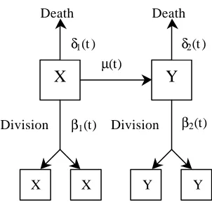
The two models are not only biologically and mathematically different but the model proposed by Leroux et al. is not a submodel of the CGD model since a linear birth process is not assumed. However, setting a specific birth, death or transformation rate to zero in the CGD model creates a model that can give similar predictions as those given by the Leroux et al. model. Specifically, consider the very simple developmental CGD model depicted in Figure 3. The system of ordinary differential equations describing the means, variances and covariances for the number of cells in states X_jand Y are given in Section A.2 of the Appendix. Using the parameters given in Table 3, the CGD and the Leroux et al. [36] model predict similar expectations albeit different variances at the time t=5(see Figure 4). Figures 5 and 6 further support the ability of the CGD model to closely parallel the Leroux

et al. model.

Table 3: Parameters Used to Predict Similar Results Among the Two Models Leroux et al. Model CGD Model

X Y X0 X1 Y

Initial number of cells (time t=0)

5

1.68 10× 0 1.68 10× 5 0 0

Birth rate, β 0.4 0.4 0.4 0.4 0.4

Death rate, δ 0.01 0.01 0.01 0.01 0.01

Expected number of cells (time t=5)

5

5.578 10× 5

6.23 10× 4

1.022 10× 5

5.476 10× 5

6.23 10×

Total number of cells 6

1.181 10× 1.181 10× 6

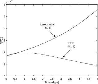
One major difference between the two models is the ability of the CGD model to deplete the population of X cells under constant rates while still maintaining the same distribution of Y cells. This can be illustrated again using the simple CGD model in Figure 3. As before, both the Leroux et al. model and the simple CGD model (Figure 3) were started with the same initial conditions. The X (Leroux et al.) and X0(CGD model) type

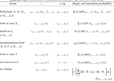
cells consisted of 1.68 10× 8cells at time t=0 while the remaining states started with a cell population of zero. The variances and covariances of each random variable were also set equal to zero at time t=0. Each model ran for a total of five time units. The set of parameter values used in the models is shown in Table 4. The only changes are setting µ₀ to zero and increasing δ₁ and µ₁.

Table 4: Parameters Used and Estimates Obtained Among the Two Models Leroux et al. Model CGD Model

X Y X0 X1 Y

Initial number of cells (time t=0)

5

1.68 10× 0 1.68 10× 5 0 0

Birth rate, β 0.4 0.4 0.4 0.4 0.4

Death rate, δ 0.01 0.01 0.01 0.4 0.01

Transformation rate, µ 0.15 -- 0 0.5174

--Expected number of cells (time t=5)

5

5.58 10× 5

6.23 10× 4

2.16 10× 4

6.69 10× 5

6.23 10×

Total number of cells 6

1.181 10× 7.115 10× 5

Figure 7 shows that the two models have the same basic density shape as before (see Figure 4) with the variance from the CGD model smaller than the variance from the Leroux

number of uncommitted cells and the birth rates in each type X population are the same. However, due to the structure of the CGD model, the state X₁cells are able to have higher death and transformation rates. Biologically, this means that all of the committed (type Y) cells have type X₁ precursor cells and that the population of uncommitted cells will eventually die out. This eventually results in a stable population of committed cells at greater times, unlike the Leroux et al. model which will continue to grow.

The expected final size of the tissue/organ is simply computed as the total number of cells present in the system at timet =5. The total number of cells, which is defined to be the sum of all expectations of type X and type Y cells, present in the Leroux et al. model exceeds the number of cells present in the CGD model. This implies that, for sufficiently large time, the size of the tissue/organ might become unrealistically large. It is also important to note that in order to reduce the number of cells in the Leroux et al. model, there are a few options available:

(i) reduce the initial number of type X cells

(ii) reduce the birth rate of the type X and/or type Y cells (iii) increase the death rate of the type X and/or type Y cells (iv) use more complicated time-varying rates

In each case, the ability to accurately reflect the biological dynamics of the development process is compromised. If options (i) or (iii) are pursued, the experimental data and the mathematical model may not agree initially. If options (ii) or (iv) are incorporated, the cellular kinetics of the system may not be modeled accurately. In any event, the end result is that the mathematical model does not realistically duplicate the biological dynamics of the system. Option (iv) requires significantly more knowledge of the time-varying nature of the developmental rates in the system.

On the other hand, the CGD model can be amended to incorporate all of the biological dynamics of the developmental process with time-constant parameters while also yielding a feasible number of cells that will ultimately dictate the expected final size of the tissue/organ. Even if the birth, death and/or transformation rates are reduced/increased in one state of the CGD model, a different state may be amended to reflect a different aspect of the system dynamics. In essence, the concept of homeostasis can be incorporated into the CGD model while still yielding biologically accurate prediction at each time step.

4. Conclusion

Due to the generalization of the CGD model, the system may be tailored to fit a host of simpler or more complicated developmental processes. Growth kinetics may be assumed to apply to both, none or a combination of the committed and uncommitted cell populations, which allows controlled growth and differentiation. The objective of such a model is to be able to predict the number of cells present in a committed state after a specified time of development. If the number of cells in the committed state is less than a specified number at a critical time, then malformation has occurred. Similarly, it is also unfavorable if there are too many cells in the committed state at a specified time of development. The CGD model has the added benefit of being able to model a biological system with the end result being a tissue/organ of realistic size. The CGD model is also able to model a wide variety of developmental systems whereas the Leroux et al. model is limited in this aspect.

Appendix

A.1 Development of the CGD model

In this section, we provide detailed calculations of the expected value of Xj, for 0,1, , 1

j= K k− . The following process can be repeated to obtain the expectations of type-Y

cells, squared expectations and the expected cross products.

Equation Section 1

(

)

1 1 0 1

0 1

0

( 1) ( , , 1, 2, , , , )

( 1) ( , , 1, 2, , , , ) ( 1) ( , , 1, 2, , , , ) ( 1) ( , , 1, , )

(

{

k

k

j j i i i i k

x x x y i

i j i j

j j j j j k

j j j j j k

j k k k

j

E X t t x x tP x x x x y t

x x tP x x x x y t

x x tP x x x x y t

x x tP x x y t

x x β β β β − + = ≠ − ≠ − − − +  + ∆ = + ∆ + −   + + ∆ + − + + ∆ + − + + ∆ + +

∑∑ ∑∑ ∑

K K K K K 0 0 1

1 1 0 1

0

0 0

1

1 1 0 1

1) ( , , 1, , , , )

( 1) ( , , 1, , , , ) ( 1) ( , , 1, , , , )

( 1) ( , , 1, , , 1, )

( 1) ( , , 1, ,

k

i i i k

i i j i j

j j j j k

j j j j k

k

j i i i k

i i j i j

j j j j k

tP x x x y t

x x tP x x x y t

x x tP x x x y t

x x tP x x x y t

x x tP x x x

δ δ δ µ µ = ≠ − ≠ − − − = ≠ − ≠ − − − + ∆ + + + ∆ + + + ∆ + + + ∆ + − + + ∆ +

∑

∑

, 1, ) ( 1) ( , , 1, , , 1, ) ( 1) ( , , , 1, )

( 1) ( , , , 1, )

1 ( ) ( ) ( , , , , ) .

}

j j j j k

j y k

j y k

k

j i i i i y y k

i

y t

x x tP x x x y t

x y tP x x y t

x y tP x x y t

x x t y t P x x y t

µ β δ β δ µ β δ = − + + ∆ + − + − ∆ − + + ∆ +   + _ − + + ∆ − + ∆ _ 

∑

We now rescale all the probability density functions and denote P x( ₀,…,x y t_k, , ) simply by

( , , ).

P x y tv (A.2)

(

)

( , , ) ( 2) ( , , )

( 1) ( , , ) ( , , ) ( , , ) ( 1) ( , , )

( 1) ( , , )

{

k

j j i i j j j

x y i

i j i j

j j j j k k

k

j i i j j j

i i j i j

j j j

j i

E X t t x x tP x y t x x tP x y t

x x tP x y t x x tP x y t

x x tP x y t x x tP x y t

x x tP x y t

x x β β β β δ δ δ − − − = ≠ − ≠ − − = ≠ − ≠  + ∆ = ∆ + + ∆   + − ∆ + ∆ + ∆ + − ∆ + − ∆ +

∑∑ ∑

∑

( , , ) ( , , ) ( 1) ( , , )

( , , ) ( , , )

( , , ) ( ) ( , , ) ( ) ( , , ) .

}

i j j j j j j

i i j i j

j y j y

k

j j i i i i j y y

i

tP x y t x x tP x y t x x tP x y t

x y tP x y t x y tP x y t

x P x y t x x tP x y t x y tP x y t

µ µ µ β δ β δ µ β δ − − = ≠ − ≠ = ∆ + ∆ + − ∆ + ∆ + ∆ + − + + ∆ − + ∆

∑

∑

v v v

v v

v v v

(A.3)

Further simplifications reduce to

1 1

[ ( )] {2 ( , , )

( ) ( , , ) ( , , )}.

j j j

x y

j j j j j

E X t t t x P x y t

t x P x y t x P x y t β β δ µ − − + ∆ = ∆ − + + ∆ +

∑∑

v v (A.4)

Recall the mathematical definition of the moments and correlations of the discrete random variables X_jand Y at time t is given by

(

)

00 10 1,0 0 0

0 1

0 0

1

, , , , , ,0 0

( ) | (0) , (0)

( , , , , , ).

k k k

n p

j j j

n p

j x x x x y k

x x x y

y

E X t t Y t t X x Y y

x P ₋ x x x y t t

 

 + ∆ + ∆ = = 

=

∑∑ ∑∑

(A.5)

(with n =1, p=0). Thus, equation (A.4) reduces to

1 1

[ ( )] 2 [ ( )]

( ) [ ( )] [ ( )].

j j j

j j j j j

E X t t t E X t

t E X t E X t

β

β δ µ

− −

+ ∆ = ∆

− + + ∆ + (A.6)

Finally, subtracting E X t[ j( )] from both sides of equation (A.6), dividing by ∆tand letting

t

∆ approaches zero to obtain

+ ∆ −

or

1 1

[ _j( )] 2 _j [ _j ( )] ( _{j j j}) [ _j( )].

d

E X t E X t E X t

dt = β − − − β +δ +µ (A.8)

A.2 Mathematical model for the CGD system shown in Figure 3

{

}

0 0 0 0 0

[ ( )] ( ) ( ) ( ) [ ( ) ]

d

E X t t t t E X t

dt = − β +δ +µ (A.9)

{

}

1 1 1 1 1 0 0

[ ( )] ( ) ( ) ( ) [ ( )] 2 ( ) [ ( )]

d

E X t t t t E X t t E X t

dt = β −δ −µ + β (A.10)

{

}

[ ( )] _y( ) _y( ) [ ( )] ( ) [ ( )] ( ) [ ( )]

d

E Y t t t E Y t t E X t t E X t

dt = β −δ +µ +µ (A.11)

{

}

{

}

2 2

0 0 0 0 0

0 0 0 0

[ ( ) ] 2 ( ) ( ) ( ) [ ( )] ( ) ( ) ( ) [ ( )]

d

E X t t t t E X t

dt

t t t E X t

β δ µ β δ µ = − + + + + + (A.12)

{

}

{

}

1 1 1 1 1

1 1 1 1

0 0 0 0 1

[ ( ) ] 2 ( ) ( ) ( ) [ ( )]

( ) ( ) ( ) [ ( )]

4 ( ) [ ( ) ] 4 ( ) [ ( ) ( )]

d

E X t t t t E X t

dt

t t t E X t

t E X t t E X t X t

β δ µ β δ µ β β = − − + + + + + (A.13)

{

}

{

}

{

}

0 0 1 1

0 0 1 1

[ ( )] 2 ( ) ( ) [ ( )] ( ) ( ) [ ( )] [ ( ) ( )] [ ( ) ( ) ]

2 [ ( ) ( ) ] [ ( ) ( )]

y y y y

d

E Y t t t E Y t t t E Y t

dt

E X t Y t E X t Y t

E X t Y t E X t Y t

β δ β δ µ µ µ µ = − + + + + + + (A.14)

{

}

0 1 0 0 0 0

1 1 1 0 0 0 0 1

[ ( ) ( )] 2 ( ) [ ( )] 2 ( ) [ ( )]

( ) ( ) ( ) ( ) ( ) ( ) [ ( ) ( )]

d

E X t X t t E X t t E X t

dt

t t t t t t E X t X t

β β β δ µ β δ µ = − + + − − − − − (A.15)

{

}

0 0 0 0 0

2

0 0 0 0 1 0 1

[ ( ) ( ) ] ( ) ( ) ( ) ( ) ( ) [ ( ) ( )]

( ) [ ( ) ] ( ) [ ( )] ( ) [ ( ) ( ) ]

y y

d

E X t Y t t t t t t E X t Y t

dt

t E X t t E X t t E X t X t

β δ β δ µ µ µ µ = − − − − − + + (A.16)

{

}

1 0 1 1 1

2

1 1 1 1

0 0 1 0 0

[ ( ) ( )] ( ) ( ) ( ) ( ) ( ) [ ( ) ( )] ( ) [ ( ) ] ( ) [ ( )]

( ) [ ( ) ( ) ] 2 [ ( ) ( )]

y y

d

E X t Y t t t t t t E X t Y t

dt

t E X t t E X t

t E X t X t E X t Y t

References

1. Wilson, JD, Biological bases for cancer dose-response extrapolation procedures.

Environ Health Perspect, 90: p. 293-6, 1991.

2. Portier, CJ, Mechanistic modelling and risk assessment. Pharmacol Toxicol, 72(Suppl 1): p. 28-32, 1993.

3. Kohn, M and Lucier, G, Mechanism-based toxicology in cancer risk assessment: biologically-based models. in 2nd World Congress on Alternatives and Animal use in the Life Sciences: Elsevier. 1997.

4. Armitage, P and Doll, R, The age distribution of cancer and a multi-stage theory of carcinogenesis. British Journal of Cancer, 8: p. 1-12, 1954.

5. Armitage, P and Doll, R, A two-stage theory of carcinogenesis in relation to the age distribution of human cancer. British Journal of Cancer, 11: p. 161-169, 1957.

6. Moolgavkar, SH, The multistage theory of carcinogenesis and the age distribution of cancer in man. J Natl Cancer Inst, 61(1): p. 49-52, 1978.

7. Moolgavkar, SH, Day, NE and Stevens, RG, Two-stage model for carcinogenesis: Epidemiology of breast cancer in females. J Natl Cancer Inst, 65(3): p. 559-69, 1980. 8. Chu, KC, A nonmathematical view of mathematical models for cancer. J Chronic

Dis, 40(Suppl 2): p. 163S-170S, 1987.

9. Moolgavkar, SH, Dewanji, A and Venzon, DJ, A stochastic two-stage model for cancer risk assessment. I. The hazard function and the probability of tumor. Risk Anal, 8(3): p. 383-92, 1988.

10. Dewanji, A, Venzon, DJ and Moolgavkar, SH, A stochastic two-stage model for cancer risk assessment. II. The number and size of premalignant clones. Risk Anal, 9(2): p. 179-87, 1989.

11. Portier, CJ and Kopp-Schneider, A, A multistage model of carcinogenesis incorporating DNA damage and repair. Risk Anal, 11(3): p. 535-43, 1991.

12. Luebeck, EG, Moolgavkar, SH, Buchmann, A and Schwarz, M, Effects of polychlorinated biphenyls in rat liver: quantitative analysis of enzyme-altered foci.

Toxicol Appl Pharmacol, 111(3): p. 469-84, 1991.

13. Kopp-Schneider, A, Portier, CJ and Sherman, CD, The exact formula for tumor incidence in the two-stage model. Risk Anal, 14(6): p. 1079-80, 1994.

14. Sherman, CD, Portier, CJ and Kopp-Schneider, A, Multistage models of carcinogenesis: an approximation for the size and number distribution of late-stage clones. Risk Anal, 14(6): p. 1039-48, 1994.

15. Kopp-Schne ider, A and Portier, CJ, A stem cell model for carcinogenesis. Math Biosci, 120(2): p. 211-32, 1994.

16. Kopp-Schneider, A and Portier, CJ, Carcinoma formation in NMRI mouse skin painting studies is a process suggesting greater than two stages. Carcinogenesis, 16(1): p. 53-9, 1995.

18. Dewanji, A, Luebeck, EG and Moolgavkar, SH, A biologically based model for the analysis of premalignant foci of arbitrary shape. Math Biosci, 135(1): p. 55-68, 1996.

19. Denes, J and Krewski, D, An exact representation for the generating function for the Moolgavkar- Venzon-Knudson two-stage model of carcinogenesis with stochastic stem cell growth. Math Biosci, 131(2): p. 185-204, 1996.

20. Kopp-Schneider, A, Portier, C and Bannasch, P, A model for hepatocarcinogenesis treating phenotypical changes in focal hepatocellular lesions as epigenetic events.

Math Biosci, 148(2): p. 181-204, 1998.

21. Sherman, CD and Portier, CJ, Multistage carcinogenesis Models, in Encyclopedia of

Biostatistics, P. Armitage and T. Colton, Editors. Wiley and Sons: Sussex, England.

p. 2808-14, 1998.

22. Portier, CJ, Sherman, CD and Kopp-Schneider, A, Calculating Tumor Incidence from Nonhomogenous Multistage Models of the Cancer Process. Risk Analysis, (submitted).

23. Portier, CJ, Kopp-Schneider, A and Sherman, CD, Calculating tumor incidence rates in stochastic models of carcinogenesis. Math Biosci, 135(2): p. 129-46, 1996.

24. El-Masri, H and Portier, CJ, Replication potential of cells via the protein kinase C-MAPK pathway: Application of a mathematical model. Bulletin of Mathematical Biology, 61(2): p. 379-398, 1999.

25. Melnick, RL, Kohn, MC and Portier, CJ, Implications for risk assessment of suggested nongenotoxic mechanisms of chemical carcinogenesis. Environ Health Perspect, 104 Suppl 1: p. 123-34, 1996.

26. Kimmel, CA, Health assessment of exposure to developmental toxicants. Dev Toxicol Environ Sci, 12: p. 39-48, 1986.

27. Kavlock, RJ and Setzer, RW, The road to embryologically based dose-response models. Environ Health Perspect, 104 Suppl 1: p. 107-21, 1996.

28. Kupper, LL, Portier, C, Ho gan, MD and Yamamoto, E, The impact of litter effects on dose-response modeling in teratology. Biometrics, 42(1): p. 85-98, 1986.

29. Ryan, L, The use of generalized estimating equations for risk assessment in developmental toxicity. Risk Anal, 12(3): p. 439-47, 1992.

30. Ryan, L, Using historical controls in the analysis of developmental toxicity data.

Biometrics, 49(4): p. 1126-35, 1993.

31. Lefkopoulou, M and Ryan, L, Global tests for multiple binary outcomes. Biometrics, 49(4): p. 975-88, 1993.

32. Carr, GJ and Portier, CJ, An evaluation of some methods for fitting dose-response models to quantal-response developmental toxicology data. Biometrics, 49(3): p. 779-91, 1993.

33. Bieler, GS and Williams, RL, Cluster sampling techniques in quantal response teratology and developmental toxicity studies. Biometrics, 51(2): p. 764-76, 1995. 34. George, EO and Bowman, D, A full likelihood procedure for analysing exchangeable

binary data. Biometrics, 51(2): p. 512-23, 1995.

35. Ten Have, TR, Kunselman, A and Zharichenko, E, Accommodating negative intracluster correlation with a mixed effects logistic model for bivariate binary data.

36. Leroux, BG, Leisenring, WM, Moolgavkar, SH and Faustman, EM, A biologically-based dose-response model for developmental toxicology. Risk Anal, 16(4): p. 449-58, 1996.

Figure 1: Developmental process of a tissue or organ as described by Leroux et al.[36]. The developmental parameters are birth (β_i( )t for i=1,2), death (δ_i( )t for i=1,2) and transformation (µ( )t ).

Figure 2: A general CGD system with k+2 states. This system allows the cells to go through various levels of maturation before committing to the differentiation process.

µ(t)

X X

X

Division β1(t) Death

δ1(t )

Y Y

Y

Division β2(t) Death

δ2(t )

βy(t)

δy(t)

Y

β1(t)

β0(t)

µ0(t) X0

δ0(t )

X1

δ1(t )

µ1(t)

βk−1(t)

βk(t)

Xk

δk(t)

Figure 3: The specific case of the CGD model when k=1. In this example, the transformation rate for the X0 state is set equal to zero; thus, only cells from the X1state

transform to the Y state. Table 3 lists all of the developmental rates associated with this particular CGD model.

Figure 4: Distribution of type Y cells at t=5 for the Leroux et al. model and the CGD model

βy(t)

δy(t)

Y

β0(t) X0

δ0(t )

µ1(t)

β1(t)

X1

δ1(t)

6.1 6.15 6.2 6.25 6.3 6.35

x 105 0

0.5 1 1.5 2 2.5x 10

-4

Number of Cells

Density

Leroux et al. (fig. 1)

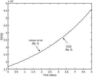
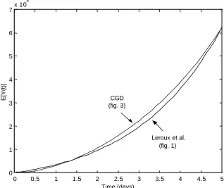
Figure 5: Expected number of type Y cells as predicted by the Leroux et al. model and the CGD model using parameters in Table 3.

Figure 6: Expected number of type X cells as predicted by the Leroux et al. model and the CGD model (E X t

[

]

0 0.5 1 1.5 2 2.5 3 3.5 4 4.5 5

0 1 2 3 4 5 6 7x 10

5

Time (days)

E[Y(t)]

Leroux et al.

(fig. 1) CGD

(fig. 3)

0 0.5 1 1.5 2 2.5 3 3.5 4 4.5 5

1.5 2 2.5 3 3.5 4 4.5 5 5.5

6x 10

5

Time (days)

E[X(t)] _{Leroux et al.}

(fig. 1)

Figure 7: Distribution of type Y cells at t=5 for the Leroux et al. model and the CGD model assuming a normal density with mean and variance derived from the first and second moments using parameters in Table 4.

0 0.5 1 1.5 2 2.5 3 3.5 4 4.5 5

0 1 2 3 4 5 6 7x 10

5

Time (days)

E[Y(t)] CGD

(fig. 3)

Leroux et al. (fig. 1)

6.1 6.15 6.2 6.25 6.3 6.35

x 105 0

0.2 0.4 0.6 0.8 1 1.2 1.4 1.6 1.8

2x 10

-4

Number of Cells

Density

CGD (fig. 3)

Figure 9: Expected number of type X cells as predicted by the Leroux et al. model and the CGD model using parameters in Table 4.

0 0.5 1 1.5 2 2.5 3 3.5 4 4.5 5

0 1 2 3 4 5 6x 10

5

Time (days)

E[X(t)]

Leroux et al. (fig. 1)