Finite Element Simulations of Shape Memory Alloy Actuators in Adaptive Structures

ABSTRACT

FRAUTSCHI, JASON PAUL. Finite Element Simulations of Shape Memory Alloy Actuators in Adaptive Structures. (Under the direction of Stefan Seelecke.)

FINITE ELEMENT SIMULATIONS OF SHAPE MEMORY ALLOY ACTUATORS IN ADAPTIVE STRUCTURES

by

JASON PAUL FRAUTSCHI

A thesis submitted to the Graduate Faculty of North Carolina State University

in partial fulfillment of the requirements for the Degree of

Master of Science

MECHANICAL AND AEROSPACE ENGINEERING Raleigh

2003

APPROVED BY:

________________________________ _________________________________ Dr. Mohammad N. Noori Dr. Ralph C. Smith

________________________________ Dr. Stefan Seelecke

PERSONAL BIOGRAPHY

Jason Paul Frautschi, born in Milwaukee, WI, obtained his Bachelor of Science degree in mechanical engineering from Temple University in Philadelphia in 2000. There, after receiving the Ennis W. Cosby faculty scholarship, he received first honors in the School of Engineering,

ACKNOWLEDGEMENTS

This research was supported by the National Science Foundation through the grant DMI-0134464.

Special thanks are due to each member of my advisory committee: Dr. Noori, for his steadfast confidence in my success at NCSU; Dr. Smith for his motivating enthusiasm and guidance; and most of all, to Dr. Seelecke, who from the moment I arrived on campus acted as a perpetual source of inspiration through his meticulous approach to science.

Thanks also to Dr. Seelecke’s other graduate students, Olaf Heintze and Jinghua Zhong, who have provided humor and camaraderie in the office.

I thank my extended family, whose curiosity in my studies and concern for my well-being have buoyed my spirits and maximized the enjoyment I have received from my work here at NCSU.

TABLE OF CONTENTS

Page

LIST OF TABLES... v

LIST OF FIGURES... vi

1. INTRODUCTION ... 1

2. SHAPE MEMORY ALLOY BEHAVIOR ... 6

2.1. SMA model... 9

2.1.1. Free energy description... 9

2.1.2. Model equations ... 21

2.1.3. Model behavior ... 26

3. FINITE ELEMENT METHOD... 30

3.1. Governing equations ... 31

3.2. ANSYS solution process ...34

4. MODEL IMPLEMENTATION ... 38

4.1. Implementation performance evaluation... 45

5. OTHER APPLICATIONS ... 59

5.1. Adaptive beam ... 59

5.2. Aerospace application... 64

5.3. Micro-actuator ... 70

6. CONCLUSION ... 73

REFERENCES:... 74

APPENDIX A: ANSYS / element data exchange... 76

APPENDIX B: usermat.F subroutine ... 79

APPENDIX C: macro pseudo-code ... 83

APPENDIX D: ANSYS solution process, force control example ... 87

LIST OF TABLES

Page

LIST OF FIGURES

Page

Figure 1: Comparison of actuation performance [1] ... 1

Figure 2: ‘Morphing Airplane' [2] ... 2

Figure 3: Flexible trailing edge of a wing actuated by SMA wires [3] ... 3

Figure 4: Shape memory effect [12]... 8

Figure 5: Helmholtz free energy density curve ... 10

Figure 6 : Gibbs free energy density function @ 293 K, no load ... 19

Figure 7 : Gibbs free energy density function @ 273 K, no load ... 20

Figure 8 : Gibbs free energy density function @ 273 K, loaded ...20

Figure 9 : Gibbs free energy density function @ 343 K, loaded ...21

Figure 10: Prescribed displacement vs. time for model behavior description ... 26

Figure 11: SMA model stress-strain curve, 273 K ... 27

Figure 12: SMA model stress-strain curve, 313 K ... 28

Figure 13: SMA model stress-strain curve, 353 K ... 29

Figure 14: Convergence criteria selection: force - displacement curves ... 36

Figure 15: SMA - spring system... 45

Figure 16: Typical strain-temperature plot in SMA-spring system... 46

Figure 17: Heat pulse applied to the SMA actuator ... 47

Figure 18: Resulting temperature history...48

Figure 19: Phase evolution ... 49

Figure 20: SMA actuator stroke vs. time...50

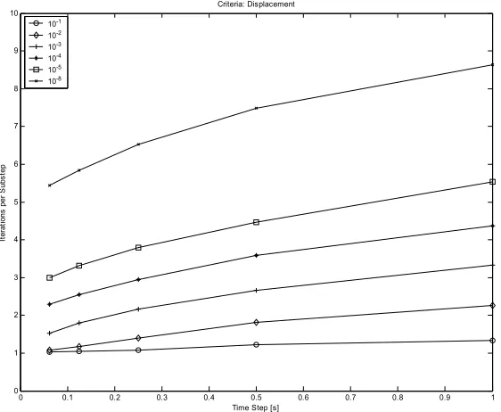
Figure 21: Iterations per time step, displacement convergence criterion ... 51

Figure 22: Iterations per time step, force convergence criterion ... 51

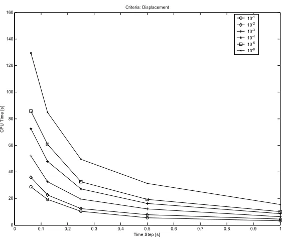
Figure 23: CPU time, displacement convergence criterion... 53

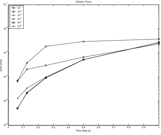
Figure 26: Averaged displacement error, force convergence criterion... 55

Figure 27: Efficiency plot, displacement convergence criterion... 57

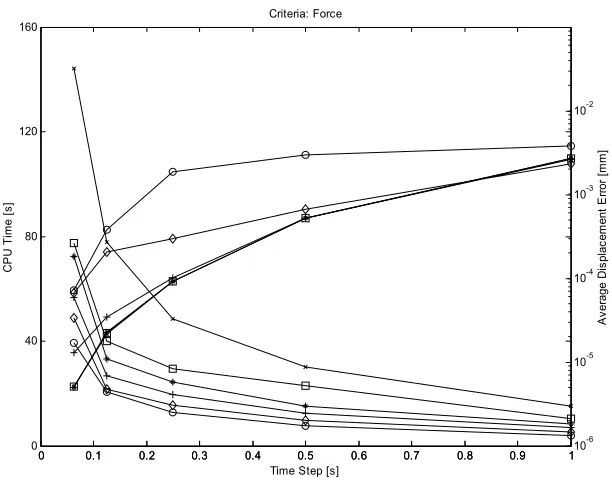
Figure 28: Efficiency plot, force convergence criterion ... 57

Figure 29: Influence of tolerance on Runge-Kutta integration scheme ... 58

Figure 30: Beam discretization ... 59

Figure 31: Beam simulation, joule heating prescription ... 60

Figure 32: Beam deflection, right wire heated ... 61

Figure 33: Beam deflection, both wires heated ... 62

Figure 34: Beam displacement, left wire cooled ... 62

Figure 35: “Smart Wing” concepts [22] ...64

Figure 36: Trailing edge discretization ... 65

Figure 37: Trailing edge joule heating input...66

Figure 38: Wing tip deflection ... 67

Figure 39: Trailing edge deformed shape, upper wires heated ... 68

Figure 40: Trailing edge deformed shape, lower wires heated... 69

Figure 41: Micro-actuator dimensions (in mm) ... 70

Figure 42: Micro-actuator, maximum displacement... 71

Figure 43: Micro-actuator, von Mises stress under maximum deformation... 72

Figure 44: ANSYS data flow chart ... 78

Figure 45: Model system, 2 links, 3 nodes, for example solution process ... 87

Figure 46: Bi-linear material behavior used in example solution process ... 87

Figure 47: Model system, 2 links, 3 nodes, for example solution process ... 94

1. INTRODUCTION

The properties of shape memory alloys (SMA) make them viable as actuators in many applications, particularly those that are weight critical, that are used in ‘clean-room’ environments, or that require a high force and high stroke under severe space restrictions. The so-called ‘shape memory’ effect, resulting from solid-solid phase transformations in the crystal lattice structure, lends these materials an inherent actuation capability combining high strains with an exceptional specific work output. Figure 1 compares SMA actuator performance with a selection of other actuation methods and materials. Shape memory alloys lead the list in maximum actuation stress and rival even hydraulics in specific work output, approaching 108 J/m3. This is the highest specific work output amongst all known smart materials.

Figure 1: Comparison of actuation performance [1]

at a number of potential fields of application for SMA actuators. For example, eliminating gear systems also obviates the need for lubricating oils that may not be compatible with ‘clean room’ environments, as well as removing the effects of gear lash and the resulting positioning

inconsistency associated with these transmission devices. Similarly, reduction of the

infrastructure needed for actuation mechanisms generates obvious benefits in weight- or space-restricted applications. For example, not only does eliminating the piping and pumping systems typical of more traditional actuation systems benefit performance through weight savings, but it also potentially liberates space in a structure, allowing modification to the structure’s configuration or providing extra housing space for additional systems. Further, the loss of piping systems precludes the need for routing cutouts in the structure, permitting structural optimization without the stress concentrations caused by these cutouts.

As a result of these attributes, potential applications for shape memory alloy actuators span the range from micro-scale positioning devices to large-scale structural actuators, in concepts as far-reaching as NASA’s ‘morphing airplane’ (Figure 2) to those already under experimental evaluation, such as the flexible wing trailing edge shown in Figure 3.

Figure 3: Flexible trailing edge of a wing actuated by SMA wires [3]

In fact, much of the development in the field of adaptive structures has been motivated by applications in aerospace engineering, where the properties of SMA actuators are particularly well-suited. These applications involve quasi-static shape control, such as the in-flight

optimization of aircraft wings for improved fuel consumption and performance. Within this arena, the aircraft industry has pursued several research projects under so-called smart wing programs organized by the Defense Advanced Research Projects Agency (DARPA), resulting in

built design iterations needed to realize an effective mechanism. Additionally, the simulations can yield insight into the behavior of a structure that may be overlooked in physical experimentation, for example where comprehensive instrumentation is cost-prohibitive or otherwise unfeasible.

For structural simulations, the most widely used tool is the finite element (FE) method. This numerical method makes analysis of arbitrary structures possible, even those having irregular shapes, known material inhomogeneities, or other features that preclude the use of classical, analytical methods. Of course, for useful, physically representative simulations, developing a characteristic material model and correctly integrating the chosen simulation solution algorithm yields the greatest possibility for meaningful simulation results. This is particularly true for shape memory alloys, which show highly nonlinear and hysteretic behavior.

Though many models for the behavior of SMAs have been developed over the past two decades, the number of implementations into a finite element framework is very small, see, e.g., [7,8]. When it comes to actuator applications, the number of suitable SMA models further

diminishes since most require direct prescription of the temperature. However, realistically, from a controls perspective the actuator temperature per se is a quantity that is both difficult to measure and impossible to instantaneously control.

More suitable would be a model that includes an energy balance for determining temperature and material behavior following from a prescribed electric current through the actuator, since the electric current is the essential control quantity for most SMA actuators. An example of such a model is Seelecke’s improved Müller-Achenbach SMA model [9]. To the best of the author’s knowledge, there has been only one publication of a SMA actuator model including an energy balance implemented into a FE code [10]. However this was an

implementation based on a dimensionless SMA model using a research FE code. Consequently, it reproduced the material behavior only qualitatively and had only very basic structural elements available to which to couple the SMA actuator element.

SMA material model and the FE solution process in order to guarantee that the relevant

2. SHAPE MEMORY ALLOY BEHAVIOR

Shape memory alloys possess highly nonlinear and hysteretic constitutive behaviors showing a strong dependence on strain, temperature, and strain rate. These distinguishing features lend these materials an inherent actuation capability, coupling high strains with a very high work output. In this chapter, the characteristic behavior of shape memory alloy is detailed and correlated to a description of the material’s Gibbs free energy, followed by an introduction to the model used in the FE implementation.

The macroscopic behavior of SMA is caused by solid-solid phase transitions in the material’s crystal lattice structure, also referred to as martensitic transformations. In the uni-dimensional case, material behavior follows free energy minimization through diffusionless transitions between the cubic austenite phase (A) and/or two martensite variants (M+ , M-), which

may be viewed as sheared lattice cells. These phase changes may result from either mechanical or thermal loading, or both, and lead to the dominant behavioral features of SMAs, including the so-called ‘shape memory’ effect. There are two characteristic states in which SMAs are found: ‘quasi-plastic’ and ‘pseudo-elastic.’ Interaction between these two conditions leads to the shape memory effect, and also lends SMA its actuation capability.

Shape memory alloys exhibit ‘quasi-plastic’ behavior when the martensite variants are the stable phases under no load, typically at low temperatures. In such a condition, stress application initially produces a linear elastic response, up to a characteristic, temperature-dependent phase transition stress. Loading above the transition stress causes substantial deformation coinciding with a phase transformation from one variant to the other (e.g. M-Æ M+).

‘quasi-plastic,’ since the material does not behave plastically in the pure sense, instead regaining its elastic nature after yielding.

SMAs behave in a ‘pseudo-elastic’ or super-elastic manner at higher temperatures, at which austenite is the stable phase under no load. Like the quasi-plastic case, initial loading produces a linear elastic response, up to a characteristic, temperature-dependent austenite-to-martensite (A Æ M) phase transition stress. Exceeding this critical stress causes a phase transformation from austenite to a martensite variant, accompanied by substantial straining. Like the quasi-plastic case, after the phase change is completed, further loading results in a

resumption of the linear elastic behavior. When the stress is reduced below a lower, martensite-to-austenite (M Æ A) transition stress, the material transforms back to austenite, i.e. the M Æ A process occurs spontaneously. Complete unloading returns the sample to its original shape as in an elastic material, tracing a hysteretic path. Total strains may be on the order of 10 %. The very high strains achievable, combined with the complete recovery to the original configuration along a hysteretic path, explains the terms ‘pseudo-elastic’ and super-elastic.

The ‘shape memory effect’ results from the interplay of these two material behaviors, as illustrated in Figure 4. Starting in a quasi-plastic state (a twinned-martensite phase composition), with variants shown in green (representing M+) and blue (representing M-), initial loading causes

existing M+ layers to stretch along their original orientation, but begins to deform the M- layers

through shearing. Loading over the transition stress causes the M- layers to lose stability and ‘flip’

into the M+ orientation. Once this has occurred, unloading leaves the material in a state of

remnant deformation since the reverse transformation does not occur spontaneously. After this plastic-like deformation in the quasi-plastic regime, the original shape may be recovered by heating the material up to the transition temperature, causing a phase transformation, whereupon the lattice cell structure shifts from the sheared martensite variant (M+ in this case) into body

simultaneous formation of the two variants of martensite, which mutually cancel their strain contributions.

Figure 4: Shape memory effect [12]

Because of the difference in stress levels that induce transformation from one phase to another (or from one martensite variant to the other), there is a very pronounced hysteresis loop during cyclical loading where phase changes occur. Such hysteresis loops dissipate energy, producing a damping effect in vibration [13]. Thus shape memory alloys used as passive elements in a structure act as both non-linear springs and passive dampers, provided strain levels are sufficiently high to induce phase transformations. In applications where the SMA is used as an active component in an adaptive structure, and where the driving frequency is significantly smaller that the structural natural frequency, the hysteresis acts as an impediment in the ability of conventional control methods to follow a set track and necessitates the use of a model-based control scheme for optimal operation, particularly at higher frequencies.

2.1. SMA model

For this implementation the model representing the constitutive stress-strain relation of the SMA actuator is Seelecke’s extension of the Müller-Achenbach model [16]. This model describes phase transformations as thermally activated processes governed by principles from statistical thermodynamics, and employs an ansatz free energy density function. A system of first-order, ordinary differential equations (ODEs) representing evolution laws for the phase fractions and temperature constitute the model.

Phase changes resulting from mechanical or thermal loading are predicted according to the fundamental quantity of interest, the Gibbs free energy, which is assumed to be described by a multi-parabolic function dependent on strain, temperature, and applied stress. Local minimum energy locations, or “wells,” for each phase are provided, as well as energy barriers between wells. Phase transitions occur when the barriers between phase-specific free energy minimums are eliminated by either mechanical or thermal loading.

In the following, after the Gibbs free energy is described, the model is introduced through a brief summary of its equations and an examination of representative plots characterizing its behavior.

2.1.1. Free energy description

Since the Gibbs free energy is the fundamental quantity in the model, it is useful to understand its form in order to comprehend the machinations of the model. Characterization of SMA behavior is attained by means of a free energy description having a hypothesized multi-parabolic shape representing the free energy density as a function of strain and temperature. At equilibrium under no load, the micro-structural phase composition may be predicted at a

This Helmholtz free energy density function, ψ, is assumed to be composed of five parabolas, one for each of the three material phases (A, M+ , M- ) and two for the energy barriers

between austenite and the two martensite phases (shown as C+ , C- in Figure 5) .

-0.06 -0.04 -0.02 0 0.02 0.04 0.06

-1.5 -1 -0.5 0 0.5 1 1.5 2 2.5

x 106

strain

M- M+

C- C+

A -wm

w_a

w_m

-w_a

-eT eT

Figure 5: Helmholtz free energy density curve

Identification of some particular points of interest in the ψ - strain curve facilitates generation of the Helmholtz free energy density function. These points include the phase minimum energy locations and the intersections of the phase and barrier parabolae as follows (refer to Figure 5):

• εT and -εT are defined to be the strains corresponding to locations of the local minimum

energy wells for the sheared M+ and M- phases, respectively. The austenitic minimum energy

well occurs at zero strain.

• strains corresponding to inflection points between the austenite phase and its energy barriers are defined as wa and –wa.

Note that the strain εT is constant for a material, whereas wA and wM depend on the relative

positions of the austenite and martensite energy minima, as well as the curvature of the parabolae.

With the supposition that each phase and energy barrier may be depicted by a parabola, then each individual parabola could be described by the standard quadratic formulation:

ψi = ai (T) * ε2 + bi (T) * ε + ci (T)

where i = {1:5} corresponding to {A, M+ , M- , C+ , C- }, respectively, the three phases and two

connecting parabolae. For generality, the coefficients are permitted to vary with temperature T. Coefficient Determination

By assigning arbitrary nominal values to the minima of the three phases, i.e. β1(T) for

austenite, β2(T) and β3(T) for martensites M+ and M- , equations for the individual phase

parabolae and barrier parabolae can be determined. These nominal values, combined with assumed continuity and smoothness between the parabolae, dictate the following required conditions:

)

(

)

,

0

(

₁

1

T

=

β

T

Ψ

(2.1.1.1)

0

) , 0 (

1

₌

∂

Ψ

∂

T

ε

(2.1.1.2)

)

(

)

,

(

₂

2

ε

T

T

=

β

T

Ψ

_(2.1.1.3)

0

) , (

2

₌

∂

Ψ

∂

T T

ε

ε

(2.1.1.4)

)

(

)

,

(

₃

3

−

ε

T

T

=

β

T

Ψ

(2.1.1.5)

0

) , (

3

₌

∂

Ψ

∂

−εT T

ε

(2.1.1.6)

)

,

(

)

,

(

₁

4

w

A

T

=

Ψ

w

A

T

Ψ

(2.1.1.7)

1 4

ε

ε

∂

Ψ

∂

=

∂

Ψ

∂

)

,

(

)

,

(

₂

4

w

M

T

=

Ψ

w

M

T

Ψ

(2.1.1.9) ) , ( 2 ) , ( 4 T w T

wM

ε

M

ε

∂

Ψ

∂

=

∂

Ψ

∂

(2.1.1.10)

)

,

(

)

,

(

₁

5

−

w

A

T

=

Ψ

−

w

A

T

Ψ

(2.1.1.11) ) , ( 1 ) , ( 5 T w T

wA − A

−

∂

Ψ

∂

=

∂

Ψ

∂

ε

ε

(2.1.1.12)

)

,

(

)

,

(

₃

5

−

w

M

T

=

Ψ

−

w

M

T

Ψ

(2.1.1.13) ) , ( 3 ) , ( 5 T w T

wM − M

−

∂

Ψ

∂

=

∂

Ψ

∂

ε

ε

(2.1.1.14)

Evaluation of the above requirements yields equations for the coefficients of the parabolae, as follows:

From 2.1.1.1: c1(T) = β1(T)

From 2.1.1.2: b1(T) = 0

From 2.1.1.3: a2(T) εT2 + b2(T) εT + c2(T) = β2(T)

From 2.1.1.4: 2 a2(T) εT + b2(T) = 0

From 2.1.1.5: a3(T) (-εT)2 + b3(T) (-εT) + c3(T) = β3(T)

From 2.1.1.6: 2 a3(T) (-εT) + b3(T) = 0

From 2.1.1.7: a4(T) wA2 + b4(T) wA + c4(T) = a1(T) wA2 + b1(T) wA + c1(T)

From 2.1.1.8: 2 a4(T) wA + b4(T) = 2 a1(T) wA + b1(T)

From 2.1.1.9: a4(T) wM2 + b4(T) wM + c4(T) = a2(T) wM2 + b2(T) wM + c2(T)

From 2.1.1.10: 2 a4(T) wM + b4(T) = 2 a2(T) wM + b2(T)

From 2.1.1.11: a5(T) (-wA)2 + b5(T) (-wA) + c5(T) = a1(T) (-wA)2 + b1(T) (-wA) + c1(T)

From 2.1.1.12: 2 a5(T) (-wA) + b5(T) = 2 a1(T) (-wA) + b1(T)

From 2.1.1.13: a5(T) (-wM)2 + b5(T) (-wM) + c5(T) = a3(T) (-wM)2 + b3(T) (-wM) + c3(T)

Since there are only fourteen equations available for the solution of the fifteen parabola coefficients, not all of the coefficients can be explicitly determined. Moreover, introduction of the strain values εT, wA, and wM, and the phase minima β1,β2, and β3 adds to the list of unknowns.

Consequently, other equations or relationships are required for a full description of the free energy curve. However, the coefficients may be solved as functions of a1(T), a2(T), a3(T), εT, wA,

wM, β1,β2, and β3, as shown below:

a4(T) = (a1(T) wA + a2(T) (εT – wM)) / (wA – wM)

a5(T) = (a1(T) wA + a3(T) (εT – wM)) / (wA – wM)

b1(T) = 0

b2(T) = - 2 a2(T) εT

b3(T) = 2 a3(T) εT

b4(T) = - 2 wA (a1(T) wM + a2(T) (εT – wM)) / (wA – wM)

b5(T) = 2 wA (a1(T) wM + a2(T) (εT – wM)) / (wA – wM)

c1(T) = β1(T)

c2(T) = a2(T) εT2 + β2(T)

c3(T) = a3(T) εT2 + β3(T)

c4(T) = wA2 (a1(T) wM + a2(T) (εT – wM)) / (wA – wM) + β1(T)

c5(T) = wA2 (a1(T) wM + a3(T) (εT – wM)) / (wA – wM) + β1(T)

c4(T) = wM2 (a1(T) wA + a2(T) (εT – wA)) / (wA – wM) + a2(T) εT2 + β2(T)

c5(T) = wM2 (a1(T) wA + a3(T) (εT – wA)) / (wA – wM) + a3(T) εT2 + β3(T)

Correlation Between Coefficients and Material Properties

du

Tds

d

or

d

du

Tds

=

+

−

=

ε

σ

ε

σ

,

(2.1.1.15)

where s is entropy, u is internal energy. By subtracting

d

( )

Ts

from both sides of the equation, a slightly modified form results, noting that

d

( )

Ts

=

Tds

+

sdT

:

( )

( )

(

u

Ts

)

d

sdT

d

or

Ts

d

du

Ts

d

Tds

d

−

=

−

−

=

−

+

ε

σ

ε

σ

,

(2.1.1.16)

Then, since by definition,

Ψ

=

u

−

Ts

, the differential of the Helmholtz free energy equation emerges:

sdT

d

d

Ψ

=

σ

ε

−

(2.1.1.17)

From this, since

ε

ε

ε

d

dT

T

d

T

∂

Ψ

∂

+

∂

Ψ

∂

=

Ψ

, then

s

T

_{ε constant}

=

−

∂

Ψ

∂

=

, and (2.1.1.18)

σ

ε

=

∂

Ψ

∂

=constant T (2.1.1.19)

The latter equation above motivates the use of an experimentally obtained stress-strain diagram to aid in the development of the free energy description. The stress-strain diagram yields the following useful information:

• EA = 2 a1(T) = modulus of the austenite phase (by noting that

A A A

E

₂ 2

ε

ε

σ

∂

Ψ

∂

=

=

∂

∂

)

• similarly, EM = 2 a2(T) = 2 a3(T) = modulus of the martensite phases

• εT = the strain level of a hypothetical, purely martensitic (M+) material at vanishing stress,

which occurs at the minimum of the M+ parabola

• wA = the strain at which the phase transition from austenite to martensite begins

• there is a loading stress at which a phase transition from austenite to martensite (+) begins (say, ‘σA’), corresponding to wA, where the material strains at a constant stress

• there is an unloading stress at which a phase transition from martensite (M+) to austenite

begins (say, ‘σM’), corresponding to wM, where the material strains at a constant stress

• the diagram is symmetric

All coefficients previously developed can be written in terms of these material properties and constants. Further, stress-strain diagrams from experiments conducted at various

temperatures reveal that the difference between σA and σM remains constant (independent of

temperature), i.e.

M A

σ

σ

−

= some constant ≡

∆

σ

(2.1.1.20)

As defined, wA and wM are intrinsically related to σA and σM; wA is the strain at which

phase transition (A Æ M+) begins and thus the point at which the stress σA is achieved, and

similarly wM marks the onset of the M+Æ A transition at σM. Consequently, wA and wM can be

represented by σA and ∆σ as follows:

( )

( )

( )

( )

T

M A M

A A A

E

T

T

w

E

T

T

w

ε

σ

σ

σ

+













−

∆

=

=

(2.1.1.21)

Relative Minimum Energies of the Phases

The two redundant expressions for c4(T) and c5(T) render relationships between β1(T)

and both β2(T) and β3(T). For example,

β1 + wA(T)2 (a1(T) wM(T) + a2(T) (εT – wM(T))) / (wA(T)– wM(T)) =

β2 + a2(T) εT2 + wM(T)2 (a1(T) wA(T) + a2(T) (εT – wA(T))) / (wA(T)– wM(T))

The crystallographic symmetry of the material implies a symmetric stress-strain diagram. This in turn suggests that the martensitic phase minimum energies β2 and β3 are equal and might

justifiably be denoted as martensitic, i.e. “βM.” Similarly, β1 might be justifiably denoted with an

austenite subscript, “βA.” Hence, considering the austenite and martensite (+) phases and

introducing ∆β≡βA - βM :

∆β = βA - βM = - a1(T) wA(T) wM(T) + a2(T) (εT – wA(T)) (εT – wM(T)) (2.1.1.22)

∆β can also be expressed in terms of the material properties and constants found from the

stress-strain diagram as follows:

∆β = 1/2 (σA2 (1/EA - 1/EM) - σA (2εT + ∆σ (1/EA - 1/EM)) + ∆σεT) (2.1.1.23)

Moreover, thermodynamic considerations motivate yet another expression for the βi, which are

sometimes also referred to as chemical free energies:

















+

−

+

−

=

reference reference

i i i

T

T

cT

T

T

c

T

s

u

(

)

ln

β

, i = 1,2,3 (2.1.1.24)

where

s1 = s(austenite) = sA,

s2,3 = s(martensite) = sM,

u1 = u(austenite) = uA, and

u2,3 = u(martensite) = uM

With the above relation and the assumption that the specific heat constant c is the same for both the austenite and martensite phases, ∆β can be rewritten as

∆β = (uA – uM) - (sA – sM) T

or, introducing ∆u ≡ uA – uM and ∆s ≡ sA – sM, simply

∆β = ∆u - ∆s T (2.1.1.25)

Internal Energy, Entropy, Loading Phase Transformation Stress, σA(T)

temperatures (i.e. some upper temperature, TU, and some lower temperature, TL) through

measurement of σA and σM (from the stress-strain diagram), ∆u and ∆s can be determined, i.e.

( )

( )

(

)

( )

_       ∆ +               − ∆ + −       − = ∆ − ∆ = ∆ T M A T U A M A U A U U E E T E E T sT u T σε σ ε σ σ β 1 1 2 1 1 2

1 2 (2.1.1.26)

and

( )

( )

(

)

( )

_       ∆ +               − ∆ + −       − = ∆ − ∆ = ∆ T M A T L A M A L A L L E E T E E T sT u T σε σ ε σ σ β 1 1 2 1 1 2

1 2 (2.1.1.27)

Then,

(

)

( )

(

)

(

( )

)

(

)

( )

( )

(

)

_                           − ∆ + − −       − − − − = ∆ M A T L A U A M A L A U A L U E E T T E E T T T T s 1 1 2 ... ... 1 1 2 1 2 2 σ ε σ σ σ σ (2.1.1.28)

and (from either of the temperatures at which ∆β is determined),

( )

(

)

( )

_       ∆ +               − ∆ + −       − + ∆ = ∆ _T M A T U A M A U A

U T _{E E} T _{E E}

sT

u σ 1 1 σ 2ε σ 1 1 σε

2

1 2 _(2.1.1.29)

Interjecting these ∆s and ∆u values into the ∆β equation, σA(T) can be found for any

temperature by using the standard quadratic formula, i.e. from

      − ∆ − ∆ − ∆       − −               − ∆ + −       − ∆ + = M A T M A M A T M A T A E E sT u E E E E E E T 1 1 2 )) ( 2 ( 1 1 4 1 1 2 1 1 2 ) ( 2 σε σ ε σ ε σ (2.1.1.30)

From the above equations and any stress-strain diagram, individual phase values of entropy and internal energy cannot be determined, and consequently values for βA and βM cannot

be determined. However, since in the assessment of relative equilibrium energy minima, the absolute values of βA and βM are irrelevant vis-a-vis the difference between them, arbitrarily

prescribing some value of entropy and internal energy for martensite and finding an offset from this in austenite is sufficient. For example, by setting sM and uM equal to zero, then

sA = ∆s and

uA = ∆u

Following from above,

βA = ∆u - ∆sT - c(T-TReference) – cTln(T/TReference) (2.1.1.31)

and

βM = - c(T-TReference) – cTln(T/TReference) (2.1.1.32)

Resulting Free Energy Descriptions

With the coefficients and material parameters developed above, a variation of the Helmholtz free energy, defined as

Ψ

ˆ

_{≡ψ - c(T-TReference) – cTln(T/TReference) (2.1.1.33)}

can be plotted as a function of strain and temperature. The definition of

Ψ

ˆ

effectively locks the minima of the martensitic phase parabolas to the abscissa and permits the austenitic energy

minimum to float in relation to the zero position. The plot of

Ψ

ˆ

shows both the relative magnitude of the austenitic energy minimum and the magnitude of the energy barrier(s) between phases.

Similarly, a modified form of the Gibbs free energy can be plotted as follows:

Qualitatively, phase transitions can be understood by examination of the Gibbs free energy function. A plot representing a typical NiTi material in the unloaded state at 293 K, at which all phases are stable, appears in Figure 6. The austenite phase sits in the zero strain well, while the martensite variants M- and M+ occupy the left- and right-side wells, respectively. No

phase transitions would occur under the shown condition since the barriers separating the three phase wells obstruct the free exchange of particles.

Figure 6 : Gibbs free energy density function @ 293 K, no load

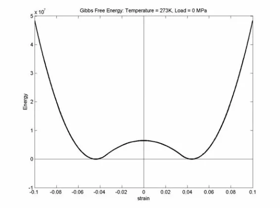
Figure 7 : Gibbs free energy density function @ 273 K, no load

The above plots show qualitatively how phase changes result from thermal loading. Under mechanical loading, the Gibbs free energy function inclines with the product of stress and strain, as shown in Figure 8. The lack of a barrier at the M - phase minimum, indicated

by the arrow, indicates a phase instability due to the accessibility of the preferable, lower energy value at the M + well. In this case, the applied stress is sufficient to cause a phase change from

one martensite variant to the other (M-Æ M+).

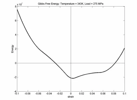
The next plot, Figure 9, shows the same material at a higher temperature under the same load. This temperature corresponds to that used to obtain Figure 6. Because of the absence of an energy barrier at the M+ well, all martensite previously formed under loading will transform into

austenite.

Figure 9 : Gibbs free energy density function @ 343 K, loaded

The last two figures demonstrate how phase changes result from the combination of both thermal and mechanical loading.

2.1.2. Model equations

Müller-Achenbach-Seelecke SMA model instead ascertains the probability that a material particle will be within a certain range of an energy well in order to predict the onset of a phase transformation according to principles from statistical thermodynamics. The transition probability for M +Æ A, for

example, is as follows:

∫











−











−

=

+

ε

σ

ε

σ

ε

π

d

kT

T

G

kT

T

G

m

kT

p

A

)

,

,

(

exp

)

,

,

ˆ

(

exp

~

2

(2.1.2.1) where,

)

,

,

(

T

G

σ

ε

is the Gibbs Free Energy function;

k

is the Boltzmann constant

ε

ˆ

is the strain that marks the onset of instability from Austenite to M+ ;

2

~

_m

_l

m

=

⋅

; where

m

is the mass of a lattice layer;

3

L

V

l

=

; where

L

V

is a representative volume.

Limits of integration follow the stable strain range for austenite. These transition probabilities are used in defining evolution laws for phase fractions, as follows:

− − − − + + + +

+

−

=

+

−

=

A A A A A A

p

x

p

x

x

p

x

p

x

x

&

&

(2.1.2.2) where +

x

_&

is the time rate of change of the fraction of the material in the M+ phase;

+

x

is the fraction of the material in the M+ phase;

A

p

+ is the transition probability for a phase transformation from M+ A (as previously

The right hand sides of the ordinary differential equations (ODE) are the weighted sums of loss- and gain-probabilities, where weighting is determined by the respective extant phase fractions. The third phase, austenite, is not represented in the phase evolution equations since there is the additional constraint that the sum of the phase fractions must be unity:

1

=

+

+

−

+

_x

_x

A

x

(2.1.2.3)

Similarly, the strain in a shape memory alloy may be written as the weighted sum of the strains in the individual phases present, as follows:

− − +

+

₊

+

=

ε

ε

ε

ε

x

A A

x

x

_(2.1.2.4)

where

ε

is strain;

A

x

is the percent of the material in the austenite phase;

A

ε

is the average strain of the austenite phase particles;

+

x

is the percent of the material in the martensite (+) phase; and so on.

The above average strain values are determined using a standard, statistical formulation as follows:

ε

ε

ε

ε

phase

f

₍

₎

d

∫

⋅

=

(2.1.2.5)

where

f

(

ε

)

marks the probability of finding a layer with a strain ‘

ε

’. In fact this is a probability

density. Limits of integration for the above equation follow the range of stable states for the particular phase, i.e. the regions of strain where the second derivative of the Helmholtz free energy density function is positive.











−

⋅

=

kT

T

G

C

f

(

ε

)

exp

(

σ

,

ε

,

)

(2.1.2.6)

where

)

,

,

(

T

G

σ

ε

is the Gibbs free energy function;

k

is the Boltzmann constant; and

C

is a constant determined from the requirement that the integral of (2.1.2.6) be unity, i.e.

∫

f

(

ε

)

d

ε

=

1

(2.1.2.7)

From this, then,

∫













=

ε

ε

σ

d

kT

T

G

C

)

,

,

(

exp

1

(2.1.2.8)

Limits of integration again follow the range of stable strains. Thus, the probability

f

(

ε

)

may be

written as

∫























−

=

ε

ε

σ

ε

σ

ε

d

kT

T

G

kT

T

G

f

)

,

,

(

exp

)

,

,

(

exp

)

(

(2.1.2.9)

And, similarly, the appropriate value for the average strain of a phase

ε

phase may be written as

∫

∫























−

=

ε

ε

σ

ε

ε

σ

ε

ε

d

kT

T

G

d

kT

T

G

phase

)

,

,

(

exp

)

,

,

(

exp

(2.1.2.10)

(

)

(

)

∫

∫

− −













−













−

=

_{( )}

) (

) (

) (

,

,

exp

,

,

exp

T w

T

w B

T w

T

w B

A a

a a

a

d

T

k

T

G

d

T

k

T

G

ε

ε

σ

ε

ε

σ

ε

ε

(2.1.2.11)

The result of the above formulation is that, given an applied stress, overall strain can be calculated provided that the material phase fractions are known. The Gibbs free energy, itself a function of strain, temperature, and applied stress, is the fundamental quantity of these integral expressions. Thus, implicit in (2.1.2.4) is the material stress-strain relationship.

Finally, the model contains a balance of energy equation for determination of temperature changes in the alloy (see Equation (2.1.2.12)). Such changes may result from heat transfer with the environment, through direct joule heating, and through latent heats absorbed and released during the phase transformations:

( )

(

₋

)

₊

( )

₋

+ +

( )

σ

₋

− −

( )

σ

=

k

T

T

t

j

t

x

H

x

H

T

mc

&

_E

_&

_&

(2.1.2.12)

This equation makes this model uniquely suitable for actuator simulation, since it draws a direct link between joule heating, which is the control quantity for most SMA actuators, and the material strain in (2.1.2.4), which is representative of the actuator stroke.

Equations (2.1.2.2) and (2.1.2.12) embody the system of ordinary differential equations that constitute the SMA model. Because this ODE system exhibits a numerically stiff behavior, an unconditionally stable implicit Runge-Kutta scheme with an adaptive time step size is used for integration. The subroutine RADAU5 was chosen for its efficiency and robustness. More details of the model can be found in [9,17].

2.1.3. Model behavior

Results of displacement controlled simulations of the SMA model at various temperatures appear in the figures below. Displacement is prescribed in the manner shown in Figure 10, except in the quasi-plastic case. Starting from an un-stretched condition, the simulated material is drawn out to some maximum extent and then permitted to return to a zero load condition. To effectively remove the self-heating and self-cooling phenomena associated with the release and absorption of latent heats, the simulation strain rate is very low, allowing ample time for temperature

equilibration. This produces a nearly isothermal response. Further, the maximum displacement is chosen to guarantee a full phase transition to M+ at full extension for the temperatures chosen.

t d

Figure 10: Prescribed displacement vs. time for model behavior description

Clearly, there is a remnant deformation as the material returns to a zero load condition, which dictates an early termination of the displacement curve of Figure 10. As shown in the figure, the initially linearly elastic material response is followed by a large displacement coinciding with a single load value, and then regains its elastic behavior on further displacement. The zero slope region of the plot corresponds to the phase transition where M- lattice layers flip to the M+

orientation. Upon unloading, these newly formed M+ layers do not retransform to their original

orientation, but instead find equilibrium in this configuration, leading to the remnant deformation. That the slope of the curve starting from the origin is the same as the slope along which the material returns to a zero load condition indicates that the initial phase composition was purely martensitic.

d

P

Figure 11: SMA model stress-strain curve, 273 K

indicates that a purely austenitic phase composition is significantly stiffer than a purely martensitic composition. Note that the load at which the A Æ M transformation occurs is higher than that shown for the quasi-plastic case. This demonstrates the model’s ability to capture the

temperature dependence of the transition stress. Once the A Æ M phase transition is complete, further deformation traces the same linear path as the lower temperature. However, as the deformation returns to zero, the material spontaneously undergoes a retransformation to

austenite at a low load level. At the end of the simulation, the material has returned to its original, un-stretched and unloaded condition, at the same time regaining a purely austenitic phase composition. The hysteresis loop circumscribed by the prescribed deformation is quite clear.

d

P

Figure 12: SMA model stress-strain curve, 313 K

The next plot shows the load-deformation curve of a simulation at yet a higher

d

P

Figure 13: SMA model stress-strain curve, 353 K

3. FINITE ELEMENT METHOD

By reducing the structural continuum into a finite number of discrete material elements for evaluation, the finite element method permits analysis of arbitrary structures, even those having irregular shapes, known material inhomogeneities, or other features that preclude the use of classical, analytical methods. The versatility of the method makes it the most widely used structural analysis tool.

After discretization, the approximate displacement of the structure at specific points (nodes) is calculated and translated by appropriate differentiation into a strain field within each element. From the strain, a stress distribution over each element is found, which, when integrated over the element, yields nodal forces. At each node, externally applied forces and nodal forces must satisfy equilibrium for a converged solution.

Because stress and stiffness of shape memory alloys depend on strain state and temperature, the global FE equations are nonlinear. Moreover, the hysteretic character of the material requires the loading to be applied incrementally through a series of time steps ∆t.

3.1. Governing equations

The global finite element equation serves as the means by which the response of any arbitrary structure can be analyzed. The weak form of the balance of momentum for the quasi-static case at time tn+1= (tn+∆t) is given by (see [18] for the derivation):

∫

(

+1

)

=

(

n+1

)

ext n

T

_σ

_a

_dv

_P

_a

B

(3.1.1)

where

B is the divergence or strain-displacement matrix,

σ is the Cauchy stress tensor,

Pext is the external loading vector, and a is displacement.

Clearly, both the stress and potentially the external loading are functions of displacement a, making this a nonlinear equation that cannot be explicitly solved, but instead requires an iterative solution method.

The Newton-Raphson iteration scheme represents the customary means of solving nonlinear equations. This scheme can be viewed as a linearization of the Taylor expansion of the equation. Let R be defined in the following way:

)

(

)

(

₊₁

−

₊₁

=

∫

ext _n

n

T

_σ

_a

_dv

_P

_a

B

R

(3.1.2)

Here, R is commonly called the ‘residual’ or ‘unbalanced’ load vector [19]. With the above definition, equation (3.1.1) becomes a homogeneous equation of the form:

0

=

R

(3.1.3)

(

( 1)

)

.

.

.

0

1 ) ( 1 ) ( 1 ) (

1

_∂

+

=

∂

+

+

+ +

+

+ i ni

h

o

t

n i n i n

a

a

R

R

δ

(3.1.4)

where ) ( 1 ) 1 ( 1 ) 1 (

1 ni ni

i

n++

=

a

++

−

a

+

a

δ

(3.1.5)

and h.o.t. are higher order terms.

Neglecting any potential changes in external loading with changes in a, and noting that

by definition

a

ε

B

∂

∂

=

, then:

∫

+ + + + + + + + + +

∂

∂

≈

∂

∂

=

∂

∂

∂

∂

=

∂

∂

dv

i n i n T i n i n i n i n i n i n i n i n

_B

ε

σ

B

B

ε

R

a

ε

ε

R

a

R

) ( 1 ) ( 1 ) ( 1 ) ( 1 ) ( 1 ) ( 1 ) ( 1 ) ( 1 ) ( 1 ) ( 1 _(3.1.6)

The integral term in the above equation is defined as the tangent stiffness:

) ( 1 ) ( 1 i n i n T

_dv

+ +

≡













∂

∂

∫

B

K

ε

σ

B

(3.1.7)

This tangent stiffness refers to the slope of the stress-strain curve at a particular strain value. For shape memory alloys, this slope ranges from values as high as the modulus of austenite (the stiffer of the phases) to near zero during stress-induced isothermal phase transitions.

Generally, then, linearizing the Taylor expansion by neglecting the higher order terms, for the i-th iteration of the time-discretized problem, the balance of momentum equation reads [20]:

(

)

() 1 1 ) 1 ( 1 ) (

1 ni next ni

i

n+

a

++

=

P

+

−

I

+

K

δ

(3.1.8)

where

I

(_ni₊)₁

≡

∫

B

T

σ

( )

a

(_ni₊)₁

dv

is the internal load vector corresponding to the internal stress state . Equation (3.1.8) reproduces the well-known Newton-Raphson iteration scheme. The equation is iterated until some convergence criterion is achieved, typically based either on a

measure of the residual force vector R or on the size of the displacement increment

δ

a

(_ni₊+₁1).

To aid in convergence behavior, a line search is used in determining the updated

displacement. This method reduces the iteration increment

δ

a

(_ni₊+₁1) in cases where the full

) 1 (

1 )

( 1 ) 1 (

1

+ + +

+

+

=

+

ni

i n i

n

a

s

a

a

δ

(3.1.9)

where 0.05 ≤ s ≤ 1 is the line search parameter.

The line search parameter s is determined by finding the solution of the equation given in [11] as:

(

)

(

( 1)

)

0

1 1

) 1 (

1

−

=

+ + +

+

+ n ni

ext T i

n

P

I

s

u

u

δ

δ

(3.1.10)

Once the line search parameter is determined, the modified iteration increment

s

δ

a

(_ni₊+₁1) is used in

the FE solution equation (3.1.8).

From this global FE equation, it is apparent that extensive communication between the global FE code and the SMA actuator model is necessary for solution. In particular, the SMA model must supply both the tangent stiffness K and the internal stress state σ for each iteration required at time tn+1 to the global FE solution algorithm, and for each iteration, the global FE code

3.2. ANSYS solution process

The general solution process used by ANSYS in the simulation of SMA actuators in adaptive structures is outlined below. In order to solve the global FE equation, ANSYS performs an iterative process, calling the SMA model several times per iteration for updating solution information until convergence is achieved.

For the first sub-step of every load step, ANSYS determines the stress state and tangent stiffness of the SMA actuators using the converged displacement solution from the final sub-step of the previous load step and a zero displacement increment:

( )

( )

(0)

1 )

0 (

1

) 0 (

1 )

0 (

1

+ +

+ +

=

=

n n

n n

a

I

I

a

σ

σ

(3.2.1)

where

a

_n(0₊)

=

a

_n

+

δ

a

_n

1 . In the case of the first sub-step of the first load step, zero displacement

and increment are assumed:

a

(₀0)

=

0

(3.2.2)

The stress and stiffness values are used to assemble the stiffness matrices and to calculate the internal restoring force vector I.

In subsequent sub-steps, stress and stiffness values corresponding to the converged solution from the previous sub-step are retained in memory, so that the initial call to the model is not required.

Together with the boundary conditions, the stiffness matrix and restoring force vector are used for determining the first iteration for the displacement increment:

( ) (

(0)

)

1 1

) 0 (

1 1

1 +

− +

+

=

n ext

−

n

n

K

P

I

a

δ

(3.2.3)

The model is called again to update the stresses based on the new strain increment, from which the residual force vector is calculated:

) 1 (

1 1 )

1 (

1 + +

+

=

−

n

ext n

n

P

I

If the convergence criteria are met, ANSYS again calls the SMA model with the

converged strain and strain increment for updated values of the stress state and tangent stiffness, and proceeds to the next sub-step. If the convergence criteria are not satisfied, then the updated stiffness and stress values are used to calculate the second displacement increment iteration,

2 1

+ n

a

δ

, and so on, until the convergence criteria are satisfied, or until the user-specified maximum

number of iterations is reached. In the event that this maximum iteration number is met, then ANSYS exits the analysis with the error that the solution did not converge.

Determination of convergence depends on the criteria specified by the user for each load step. Choices include force convergence criterion, displacement convergence criterion, or a combination of the two. Within each criterion, a convergence tolerance must be prescribed to define the extent to which the solution must meet its criteria.

The force-based convergence method compares the residual force vector with a force criterion value. Specifically, for each iteration, a reference value is calculated from the square root sum of the squares of the applied force vector and the components of the residual force vector that correspond to constrained nodes:

( )

2

( )

₍₎ 2 )

(

₌

∑

₊

∑

k i k j

ext j i

ref

P

R

F

(3.2.5)

where j encompasses all nodes and k denotes constrained nodes only. The product of this reference value and the specified convergence tolerance marks the force convergence criterion:

cnvtol

F

F

i

ref i

criterion()

=

() (3.2.6)

To this, ANSYS compares a force convergence value, which is determined from the square root sum of the squares of the components of the residual force vector corresponding to degrees of freedom:

( )

₍₎ 2 )

(

₌

∑

l i l i

val

R

F

(3.2.7)

The force convergence method is suited to instances where the slope of the load-deformation curve is steep near the strain increment in question. In this case, small changes in the displacement correspond to relatively large changes in the force, as illustrated by the red dashed curve in Figure 14; in this way the force provides a more sensitive measure of convergence than displacement.

d

P

Figure 14: Convergence criteria selection: force - displacement curves

The blue curve in the figure represents an instance where the displacement based convergence method may be more suitable. Here a relatively small change in the force corresponds to a large change in the displacement, indicating a poor sensitivity in the force. Using the force convergence method in this case introduces the possibility for a potentially large error, since the range of force values satisfying convergence may permit an unacceptably large range of corresponding displacements.

convergence criterion is the product of the reference value and the specified convergence tolerance:

( )

( )

cnvtol

u

u

a

a

a

u

i ref i criterion j i j j i j i j i ref ) ( ) ( 2 ) ( ) ( ) ( ) (

max

min

=





































=

∑

∑

(3.2.8)

The displacement convergence value is determined from the L2 norm of the displacement increment:

( )

∑

=

j i j i val

a

u

()

_δ

() 2 _(3.2.9)

When the displacement convergence value is less than the convergence criterion, then the solution is considered converged.

A combination of both force and displacement convergence criteria results in the requirement that both criteria be met for convergence, i.e.

) ( ) ( ) ( )

(

_&

i

criterion i val i criterion i

val

F

u

u

F

≤

≤

(3.2.10)

The solution process is illustrated in detail for a model problem in Appendices D and E, for both force driven and displacement driven cases, respectively.

4. MODEL IMPLEMENTATION

As previously noted, it is evident from the global FE equation that solution data must be communicated back and forth between the FE level and the model or element level. In particular, element stiffness and stresses must be available to the FE code from the SMA model, which in turn requires updated values of time and strain increments, as well as current phase composition and temperature. The commercial finite element code ANSYS was chosen for the implementation of the SMA model largely for the flexibility it provides in defining the necessary links between the FE level equation and the local material constitutive law.

Specifically, this preprocessing, solution, and post-processing software package includes a family of elements, the 18x series, that are readily modified for user-defined subroutines through an element option called ‘usermat.’ ANSYS is also attractive because of its extensive element library, nearly two hundred element types, which permits analysis of a wide array of systems ranging from structural, thermal, electromagnetic, and coupled-field systems. This coupled-field capability is especially attractive since it has the ability to handle multi-physics problems, like coupled heat transfer and mechanics. Both of these fields play an integral role in the behavior of SMA, as indicated by the nature of the ODE system that constitutes the SMA model. For the current implementation, however, ANSYS provides only structural results. Since heat transfer and temperature evolution are calculated at the model level, outside the FE

framework, this implementation should be regarded as a preliminary step towards a multi-physics implementation.

To represent a SMA actuator, a three-dimensional link element (type LINK180) was modified via the usermat option to reproduce the material behavior defined in the

reformulate it from a program to a subroutine and to correctly interpret input from the usermat subroutine. Also, a macro was written that, in addition to all the modeling, solution, and post-processing steps needed in any typical analysis, specifies SMA material parameters and joule heating prescription. Details of the subroutines are discussed below.

usermat subroutine

In an effort to use the material model as a separate, self-contained core subroutine, the usermat subroutine functions primarily as the communication link between ANSYS and the SMA

model. This practice is intended to facilitate updating the model with incremental improvements as they evolve without imposing the need to completely dissect the implementation.

Input and output data delivered to usermat and expected by the global FE code are listed and briefly explained in Appendix A. The primary data include the material parameters, state variables, strain and strain increment, and time and time increment.

A second function of the usermat subroutine is to explicitly calculate the material tangent stiffness. This can be accomplished analytically by finding the full derivative of the stress. The expression for stress is:

(

)

(

)

(

+ −

)

− +

− +

+

+

+

+

−

−

=

x

x

E

E

x

x

x

x

E

A M

T M

1

ε

ε

σ

(4.1)

where

σ is stress,

ε is strain,

εT is the zero stress strain associated with a purely M+ phase composition

Em is the martensitic elastic modulus

EA is the austenitic elastic modulus