Viscosities and Densities of Some Multi-Component Regular Liquid Solutions at Different Temperature Levels

(1)

Scholarship at UWindsor

Electronic Theses and Dissertations Theses, Dissertations, and Major Papers

2010

Viscosities and Densities of Some Multi-Component Regular

Liquid Solutions at Different Temperature Levels

Hanan El-Sayed Moussa El-Sayed

University of Windsor

Follow this and additional works at: https://scholar.uwindsor.ca/etd

Recommended Citation Recommended Citation

El-Sayed, Hanan El-Sayed Moussa, "Viscosities and Densities of Some Multi-Component Regular Liquid Solutions at Different Temperature Levels" (2010). Electronic Theses and Dissertations. 406.

https://scholar.uwindsor.ca/etd/406

This online database contains the full-text of PhD dissertations and Masters’ theses of University of Windsor students from 1954 forward. These documents are made available for personal study and research purposes only, in accordance with the Canadian Copyright Act and the Creative Commons license—CC BY-NC-ND (Attribution, Non-Commercial, No Derivative Works). Under this license, works must always be attributed to the copyright holder (original author), cannot be used for any commercial purposes, and may not be altered. Any other use would require the permission of the copyright holder. Students may inquire about withdrawing their dissertation and/or thesis from this database. For additional inquiries, please contact the repository administrator via email

(2)

Liquid Solutions at Different Temperature Levels

By

Hanan El-Sayed Moussa El-Sayed

A Dissertation

Submitted to the Faculty of Graduate Studies

through the Environmental Engineering Program

in Partial Fulfillment of the Requirements for

the Degree of Doctor of Philosophy at the

University of Windsor

Windsor, Ontario, Canada

2009

(3)

Different Temperature Levels

By

Hanan El-Sayed Moussa El-Sayed

APPROVED BY:

_______________________________ _______________________

Dr. Abdul-Fattah A. Asfour, Advisor Dr. Ali ElKamel, External Examiner Department of Civil and Environmental Engineering. Department of Chemical Engineering

University of Waterloo.

_______________________________ _________________________

Dr. Tirupati Bolisetti Dr. Ahmed Tawfik, Co-advisor

Department of Civil and Environmental Engineering. School of Computer Science

_______________________________

Dr. Rupp Carriveau Dr. Nader Zamani

Department of Civil and Environmental Engineering Department of Mechanical, Automotive, and Materials Engineering

_____________________ Dr. S. Chowdhury, Chair of Defence

(4)

iii

Author’s Declaration of Originality

I hereby certify that I am the sole author of this thesis and that no part of this

thesis has been published or submitted for publication.

I certify that, to the best of my knowledge, my thesis does not infringe upon

anyone’s copyright nor violate any proprietary rights and that any ideas, techniques,

quotations, or any other material from the work of other people included in my thesis,

published or otherwise, are fully acknowledged in accordance with the standard

referencing practices. Furthermore, to the extent that I have included copyrighted

material that surpasses the bounds of fair dealing within the meaning of the Canada

Copyright Act, I certify that I have obtained a written permission from the copyright

owner(s) to include such material(s) in my thesis and have included copies of such

copyright clearances to my appendix.

I declare that this is a true copy of my thesis, including any final revisions, as

approved by my thesis committee and the Graduate Studies office, and that this thesis has

(5)

iv

ABSTRACT

The densities and kinematic viscosities of the quinary regular system: benzene (1)

+ toluene (2) + ethylbenzene (3) + heptane (4) + cyclooctane (5) and all its corresponding

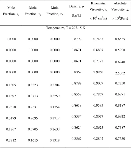
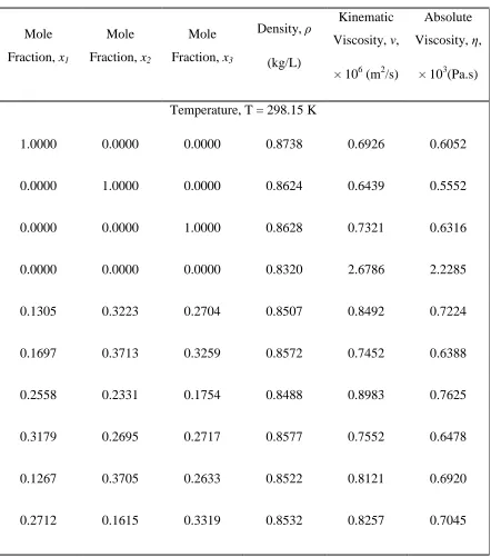
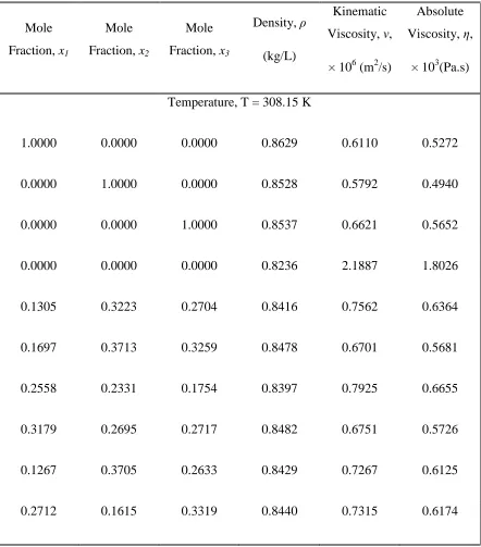
quaternary, ternary, and binary sub-systems have been measured at 293.15 K, 298.15 K,

308.15 K, and 313.15 K over the entire composition range. The experimental data

reported herein are considered valuable additions to the literature.

The experimental data gathered in the present study were utilized in testing the

predictive capabilities of some well know viscosity models available in the literature. In

addition, a new multi-layer artificial neural network (ANN) has been developed for the

prediction of the kinematic viscosities of multi-component regular liquid mixtures. The

concept of modular neural networks has been successfully applied to the design of the

current network. Only a part of the experimental binary data was required for the training

of the developed network. The remaining data on the binary systems were used for

testing the ANN-based model.

The developed neural network resulted in excellent viscosity predictions for the

cyclooctane-containing systems. The predictive capability of the ANN in the case of the

cyclooctane-containing systems was superior to the predictive capabilities of the other

tested models for all systems.

The predictive version of the McAllister three-body interaction model was the

best to predict the kinematic viscosities of non-cyclooctane-containing systems. The

predictive version of the McAllister three-body model worked very well when the

(6)

v

The reliable and accurate data resulting from the present study helped in both

critically testing existing viscosity models and in developing a new model that is based

on the ANN. Results of the present study are promising for continued work in the same

(7)

vi

DEDICATION

This thesis is dedicated to my parents who have given and are still giving me

unlimited help and support. To them I shall always be grateful. Thank you for your

(8)

vii

ACKNOWLEDGEMENTS

I would like to, first and always, express all praise and thanks to HIS

ALMIGHTY, ALLAH, who gave me the strength and energy to start and complete the

present study.

I shall be forever grateful to my supervisor Dr. Abdul-Fattah Asfour, for

suggesting the topic of this work. I will never forget his continuous support,

encouragement, and valuable guidance throughout the course of the present study.

I would like to express my sincere appreciation to Dr. Ahmed Tawfik for his

valuable assistance during the development of the neural network. His patience and

expertise in the field have resulted in a successful model.

My deep appreciation goes to the National Research Center in Egypt for the

financial support. To all my professors in the Mechanical Engineering Department for

nominating me to an Egyptian Government Scholarship and for their continuous support

all these years.

My thanks also go to Mr. Bill Middleton for his help and cooperation during the

experimental phase of my work.

I would like also to thank all my colleagues in the Environmental Engineering

(9)

viii

I would like to thank all my friends here in Windsor, Ontario who were always

present at the time of need. They helped me a lot to adapt to life abroad.

At last, but by no means least; I am deeply indebted to my beloved kids Yomna

and Mostafa who showed great patience and understanding during the years of the

present study. I would also like to thank my husband khaled for his support and

sacrifices. Finally, the motivations and wishes of all my family members played an

(10)

ix

LIST OF TABLES

Table 2.1: Different Types of interactions in a binary mixture of molecules 1 and 2, their

corresponding free energy of activation and their total of fractional occurrences

(Three-Body Interaction Model) ... 17

Table 2.2: Different Types of interactions in a binary mixture of molecules 1 and 2, their corresponding free energy of activation and their total of fractional occurrences (Four-Body Interaction Model) ... 22

Table 3.1: Specifications of the Chemicals used in the Present Study ... 82

Table 4.1: List of Systems Investigated in the Present Study ... 93

Table 4.2: Density Meter Calibration Data ... 95

Table 4.3: Viscometers Calibration Data ... 97

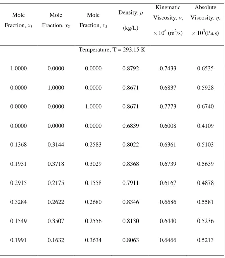
Table 4.4: Density, Kinematic Viscosity, and Absolute Viscosity-Composition Data for the Quinary System; Benzene (1) + Toluene (2) + Ethylbenzene (3) + Heptane (4) + Cyclooctane (5). ... 102

Table 4.5: Density, Kinematic Viscosity, and Absolute Viscosity-Composition Data for the Quaternary System: Benzene (1) + Toluene (2) + Ethylbenzene (3) + Cyclooctane (4). ... 106

Table 4.6: Density, Kinematic Viscosity, and Absolute Viscosity-Composition Data for the Quaternary System: Benzene (1) + Toluene (2) + Ethylbenzene (3) + Heptane (4)... 110

(14)

xiii

Table 4.8: Density, Kinematic Viscosity, and Absolute Viscosity-Composition Data for

the Quaternary System: Benzene (1) + Ethylbenzene (2) + Heptane (3) +

Cyclooctane (4). ... 118

the Quaternary System: Benzene (1) + Toluene (2) + Heptane (3) + Cyclooctane (4).

... 122

the Ternary System: Benzene (1) + Toluene (2) + Heptane (3). ... 126

Table 4.11: Density, Kinematic Viscosity, and Absolute Viscosity-Composition Data

for the Ternary System: Benzene (1) + Ethylbenzene (2) + Heptane (3). ... 130

for the Ternary System: Toluene (1) + Ethylbenzene (2) + Heptane (3). ... 134

for the Ternary System: Benzene (1) + Toluene (2) + Ethylbenzene (3). ... 138

the Ternary System: Benzene (1) + Toluene (2) + Cyclooctane (3). ... 142

for the Ternary System: Toluene (1) + Ethylbenzene (2) + Cyclooctane (3). ... 146

for the Ternary System: Benzene (1) + Ethylbenzene (2) + Cyclooctane (3). ... 150

(15)

xiv

Table 4. 18: Density, Kinematic Viscosity, and Absolute Viscosity-Composition Data

for the Ternary System: Toluene (1) + Heptane (2) + Cyclooctane (3). ... 158

for the Ternary System: Ethylbenzene (1) + Heptane (2) + Cyclooctane (3). ... 162

for the Binary System: Benzene (1) + Toluene (2). ... 166

for the Binary System: Toluene (1) + Ethylbenzene (2). ... 170

for the Binary System: Heptane (1) + Toluene (2). ... 174

for the Binary System: Heptane (1) + Ethylbenzene (2). ... 178

the Binary System: Benzene (1) + Ethylbenzene (2). ... 182

the Binary System: Benzene (1) + Heptane (2). ... 186

for the Binary System: Benzene (1) + Cyclooctane (2)... 190

for the Binary System: Toluene (1) + Cyclooctane (2). ... 194

(16)

xv

for the Binary System: Heptane (1) + Cyclooctane (2). ... 202

Table 5.1: Physical Properties of Pure Components at 293.15 K. ... 210

Table 5.2: Effective Carbon Numbers of the Pure Components as Calculated From

Equation (5.10). ... 218

Table 5.3: Results of Testing the Predictive Version of McAllister’s Three-body

Interaction Model for the Binary Sub-Systems of the Quinary System: benzene +

toluene + ethylbenzene + heptane + cyclooctane. ... 221

Table 5.4: Effect of Cyclooctane Effective Carbon Number (ECN) Change on the

Predictive Capability of McAllister Model for Binary Systems. ... 223

Table 5.5: Results of Testing the Predictive Version of the McAllister’s three-body

Interaction Model for the Ternary Sub-Systems of the Quinary System: benzene +

Predictive Capability of McAllister Model for Ternary Systems. ... 226

Interaction Model for the Quaternary Sub-Systems of the Quinary System: benzene

+ toluene + ethylbenzene + heptane + cyclooctane. ... 227

Predictive Capability of McAllister’s Model for Quaternary Systems. ... 229

(17)

xvi

heptane + cyclooctane and the Effect of Cyclooctane Effective Carbon Number

(ECN) Change... 230

Table 5.10: Physical and Critical Properties of Pure Components of the Quinary System:

benzene + toluene + ethylbenzene + heptane + cyclooctane*. ... 233

Table 5.11: Results of Testing the Predictive Capability of the GCSP Model for the

Binary Sub-Systems of the Quinary System: benzene + toluene + ethylbenzene +

heptane + cyclooctane. ... 234

Ternary Sub-Systems of the Quinary System: benzene + toluene + ethylbenzene +

heptane + cyclooctane. ... 236

Quaternary Sub-Systems of the Quinary System: benzene + toluene + ethylbenzene

+ heptane + cyclooctane. ... 238

Quinary System: benzene + toluene + ethylbenzene + heptane + cyclooctane ... 240

Table 5.15: The contribution of the Different Chemical Groups Involved in the Pure

Components of the Quinary System; benzene + toluene + ethylbenzene + heptane +

cyclooctane for the GC-UNIMOD Method* ... 243

Table 5.16: Results of Testing the Predictive Capability of the GC-UNIMOD Model for

the Binary Sub-Systems of the Quinary System: benzene + toluene + ethylbenzene +

(18)

xvii

Table 5.17: Results of Testing the Predictive Capability of the GC-UNIMOD Model for

the Ternary Sub-Systems of the Quinary System: benzene + toluene + ethylbenzene

+ heptane + cyclooctane. ... 249

the Quaternary Sub-Systems of the Quinary System: benzene + toluene +

ethylbenzene + heptane + cyclooctane. ... 251

the Quinary System: benzene + toluene + ethylbenzene + heptane + cyclooctane.

... 253

Table 5.20: Results of Testing the Predictive Capability of the Allan and Teja

Correlation for the Binary Sub-Systems of the Quinary System: benzene + toluene +

ethylbenzene + heptane + cyclooctane. ... 254

Correlation for the Ternary Sub-Systems of the Quinary System: benzene + toluene

+ ethylbenzene + heptane + cyclooctane. ... 257

Correlation for the Quaternary Sub-Systems of the Quinary System: benzene +

Correlation for the Quinary System: benzene + toluene + ethylbenzene + heptane +

(19)

xviii

Table 5.24: Results of Testing the Artificial Neural Network Model for the Binary

Sub-Systems of the Quinary System: benzene + toluene + ethylbenzene + heptane +

cyclooctane; (non-cyclooctane containing systems). ... 268

Table 5.25: Results of Testing the Artificial Neural Network Model for the Binary

Sub-Systems of the Quinary System: benzene + toluene + ethylbenzene + heptane +

cyclooctane; (cyclooctane containing systems). ... 269

Table 5.26: Results of Testing the Artificial Neural Network Model for the Ternary

non-cyclooctane containing Sub-Systems of the Quinary System: benzene + toluene

+ ethylbenzene + heptane + cyclooctane; Combination 1: AB C. ... 271

Table 5.27: Results of Testing the Artificial Neural Network Model for the Ternary

(non-cyclooctane containing) Sub-Systems of the Quinary System: benzene +

toluene + ethylbenzene + heptane + cyclooctane; average of the three combinations.

... 275

Table 5.28: Results of Testing the Artificial Neural Network Model for the Ternary

(cyclooctane containing) Sub-Systems of the Quinary System: benzene + toluene +

ethylbenzene + heptane + cyclooctane; Combination 1: AB C. ... 276

Table 5.29: Results of Testing the Artificial Neural Network Model for the Quaternary

(non-cyclooctane containing) Sub-System of the Quinary System: benzene + toluene

+ ethylbenzene + heptane + cyclooctane; Combination BC D A. ... 280

Table 5.30: Results of Testing the Artificial Neural Network Model for the Quaternary

(cyclooctane containing) Sub-System of the Quinary System: benzene + toluene +

(20)

xix

Table 5.31: Results of Testing the Artificial Neural Network Model for the Quinary

System: benzene + toluene + ethylbenzene + heptane + cyclooctane; Combination

(21)

xx

LIST OF FIGURES

Figure 2.1: The Eyring Molecular Model of Liquid Viscosity ... 13

Figure 2.2: Different Types of Molecular Interactions Involved in Binary Mixtures (Three-Body Interaction Model) ... 16

Figure 2.3: Lumped Parameters, ₁_/₃ 2 2 1 12 , Variation With (1/T) or n-alkane Systems (For which N₂ N₁ 3, Asfour et al. (1991) ... 24

Figure 2.4: Lumped Parameter Variations, ₁_/₃ 2 2 1 12 , with ₁_/₃ 2 2 1 2 1 2 N N N N For n- alkane Systems (Asfour et al.(1991), Legends are the same as indicated in Figure 2.3) ... 25

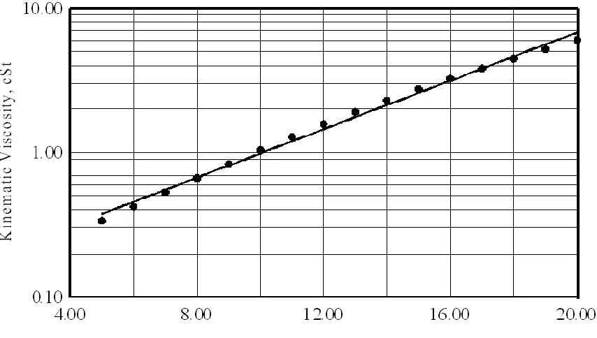
Figure 2.5: Experimental Values of Kinematic Viscosities of n-alkane Systems at 308.15 K Versus Effective Carbon Number (Nhaesi and Asfour 1998). ... 28

Figure 2.6: Different Types of Molecular Interactions Encountered with Ternary Systems (Three-Body Interaction Model, Kalidas et al. (1964)) ... 30

Figure 2.7a: Single-Layer Feed-Forward Network ... 72

Figure 2.7b: Multi-Layer Feed-Forward Network with One Hidden Layer... 72

Figure 2.8: Single-Layer Recurrent Network………...74

Figure 2.9a: A schematic Diagram Showing the Forward Phase in the Back-propagation Neural Network. ... 76

Figure 2.9b: A schematic Diagram Showing the Backward Phase in the Back-propagation Neural Network. ... 76

(22)

xxi

Figure 3.2: The Cannon-Ubbelohde Viscometer ... 88

Figure 3.3: Pictorial View of the Constant Temperature Bath ... 90

Figure 5.1: The Architecture of One Modular Network for a Binary System ... 263

Figure 5.2: A Block Diagram for the Ternary Modular Network ... 265

Figure 5.3: Predictive Capabilities of the Various Viscosity Models for Binary

non-cyclooctane Containing Systems ... 284

Figure 5.4: Predictive Capabilities of the Various Viscosity Models for Binary

Cyclooctane Containing Systems. ... 285

Figure 5.5: Predictive Capabilities of the Various Viscosity Models for Ternary

non-cyclooctane Containing Systems. ... 286

Figure 5.6: Predictive Capabilities of the Various Viscosity Models for Ternary

Figure 5.7: Predictive Capabilities of the Various Viscosity Models for Quaternary

System; benzene + toluene + ethylbenzene + heptane + cyclooctane ... 290

Figure 5.10: Predictive Capabilities of the Various Viscosity Models for

Figure 5.11: Predictive Capabilities of the Various Viscosity Models for Cyclooctane

(23)

CHAPTER 1 INTRODUCTION

1.1 General

Viscosity is an important physical property which characterizes a simple fluid’s

resistance to flow. Fluids are classified either as Newtonian fluids or non-Newtonian

fluids. Newtonian fluids are defined as those fluids that obey Newton’s law of viscosity.

Obviously, non-Newtonian fluids do not obey that law. According to Newton’s law of

viscosity, the absolute viscosity is a proportionality constant in an equation that relates

the shear stress and the shear rate, or velocity gradient. Newton’s law is given by,

dy dv

- (1.1)

The shear stress, τ, appearing in equation (1.1) is the force applied to the fluid per unit

area.

Viscosities of liquid mixtures are required in many engineering applications

involving mass and heat transfer processes. Accurate viscosity data are needed for the

design of most of fluid flow equipment.

The almost complete lack of knowledge regarding the structure of liquids and the

complex nature of, and the little knowledge we currently have about the intermolecular

forces in liquid systems, immensely contribute to the current unsatisfactory

(24)

Asfour (1979), during his study of diffusion in liquid mixtures, suggested

breaking down liquid mixtures into three categories; viz., (i) n-alkane solutions, (ii)

regular mixtures, and (iii) associated solutions. Such a classification has led to success

by Asfour (1979), Asfour (1985), Asfour and Dullien (1981), Dullien and Asfour (1985),

Asfour and Dullien (1986) in dealing with the diffusion in liquids problem. Asfour et al.

(1991) proposed extending that classification to the study of viscosities of liquid systems.

Asfour and co-workers were met with a great deal of success when they extended the

Asfour (1979) classification of liquid systems to the study of viscosity of liquid mixtures;

e.g., Asfour et al. (1991), Wu and Asfour (1992), Nhaesi and Asfour (1998), Nhaesi and

Asfour (2000a and b), and Nhaesi, et al. (2005).

Models available in the literature for calculating the viscosities of liquid mixtures

may be divided into two categories; viz., correlative or predictive. Correlative models

contain adjustable parameters whose values are determined from fitting those models to

experimental mixture data. Predictive models employ molecular properties for the

prediction of the dependence of a physical property, e.g., viscosity on composition. The

predictive models can further be classified into either semi-theoretical or empirical. The

former are normally developed on some theoretical basis and require limited

experimental data; e.g., pure component properties for the prediction of the physical

property of interest on composition. The latter employ experimental data for developing

those models.

In the present study, four well known viscosity models were subjected to testing

of their predictive capability. The selected models cover both categories; i.e.

(25)

predictive version of the generalized McAllister’s three-body interaction model, (ii) a

generalized corresponding states principle GCSP, (iii) a group contribution

GC-UNIMOD model, and (iv) the Allan and Teja correlation. In addition, an artificial neural

network based model has been developed and used for predicting the kinematic viscosity

of the investigated systems. Results from the neural network are reported and compared

to the results obtained from the remaining models. Experimental data at different

temperature levels obtained during the current study were utilized in testing the

above-named models.

McAllister (1960) utilized Eyring’s absolute rate theory to develop a correlative

model for calculating the dependence of the kinematic viscosity of liquid binary mixtures

on composition. The McAllister model was extended by Chandramouli and Laddha

(1963) to ternary liquid systems. The McAllister equation contains adjustable parameters

that require costly and time consuming experimental data for determining their values.

The correlative nature of the McAllister model drastically limits its use.

In order to overcome this problem, Asfour et al. (1991) proposed a technique for

predicting the McAllister model parameters for the case of n-alkane binary mixtures

using pure component viscosities and molecular parameters. This in effect successfully

converted the McAllister model from being a correlative model to a predictive model.

This evidently makes the McAllister, in its new form, much more useful than before.

Nhaesi and Afour (1998) extended the Asfour et al. (1991) technique to include

binary and ternary regular solutions. Following that, Nhaesi and Asfour (2000b) reported

(26)

of multi-component liquid mixtures. The model has been tested by other researchers; e.g.

Giner et al. (2006) and Bandres et al. (2009) and proved to be successful.

The Generalized Corresponding States Principle (GCSP) was first developed by

Teja and Rice (1981) for the prediction of the viscosities of multi-component n-alkane

liquid systems.. Their method requires the knowledge of the critical properties of pure

components and the concept of the reference fluid. The problem encountered with the

application of the GCSP method for mixtures of more than two components is the proper

choice of the reference fluids. It was shown by Wu and Asfour (1992) in their study of n

-alkane mixtures that the results significantly depended on the different reference fluid

combinations. There was no optimum selection reported by Teja and Rice (1981) for the

choice of the best reference fluid combination. Wu and Asfour (1992) overcame the

problem of the reference fluid selection by proposing a “pseudo-binary” model that they

incorporated into the GCSP and called their method the modified GCSP (MGCSP). The

incorporation of the “pseudo-binary” model proposed by Wu and Asfour (1992) resulted

in a method, the MGCSP, where the results did not depend on the selection of the

reference fluids, especially for the case of multi-component liquid system (Wu et al.

1998). The MGCSP was successfully extended by Nhaesi and Asfour (2000a) to include

multi-component regular solutions.

A Group Contribution GC-UNIMOD was proposed by Cao et al. (1992), (1993a),

and (1993b) is a modified version of the original group contribution approach first

developed by Langmuir (1925). The theoretical basis for that method assumes that the

(27)

made by the different chemical groups contained in that compound. Moreover, the

contribution of one chemical group is independent of the contribution of other groups.

The GC-UNIMOD assumes that the contribution of one chemical group in one

component is the same as it is in all other components. Evidently, this is not a good

assumption and there are no theoretical or experimental evidence that supports such an

assumption. This, obviously, does not make that method very reliable.

Allan and Teja (1991) reported their Antoine-type equation for viscosity of liquid

mixtures. That equation mainly depends on the number of carbon atoms contained in the

pure components constituting a mixture. The trial and error procedure involved in the

calculation of the effective carbon number of any component in the mixture in the Allan

and Teja correlation is rather cumbersome and is time consuming. This dramatically

limited the applicability of that method.

The artificial neural network has been considered in the present study due to its

fast computation as well as for its ability to successfully represent the highly non-linear

relationships involved; i.e., the viscosity-composition relationship. In the present study,

an artificial neural network using back-propagation learning algorithm has been

developed. The network was trained on only half of the reported data on binary systems.

Then the network was tested and generalized to predict the kinematic viscosities of the

quinary regular system and all the corresponding quaternary, ternary, and binary

sub-systems involved in the present study. Results of the network are reported and compared

(28)

1.2 Objectives

The present study is part of an on-going research program in our laboratory

aiming at building up an extensive database for viscosity-composition data at different

temperatures of liquid systems containing components with different chemical structures

and molecular sizes.

The primary objective of the present work is to experimentally measure and

report: (i) the densities, kinematic viscosities, and absolute viscosities of the pure

components constituting the systems under investigation, and (ii) the dependence of the

densities and viscosities of the quinary regular system: benzene (1) + toluene (2) +

ethylbenzene (3) + heptanes (4) + cyclooctane (5), and its corresponding quaternary,

ternary, and binary sub-systems on concentration, over the entire composition range, at

the temperatures of 293.15 K, 298.15 K, 308.15 K, and 313.15 K. The present study also

aims at:

(a) Employing the experimental data gathered in the present investigation to

critically test some of the viscosity models available in the literature.

(b) Developing an artificial neural network for predicting the viscosities of

multi-component regular liquid systems using part of the reported

experimental data, and using the other part of the data for validating the

model.

(29)

1.3 Contributions and Significance

Viscosities of liquid mixtures are required in many engineering applications.

However, costly and time consuming experiments are required in order to collect such

data. In addition, data on the viscosities of multi-component liquid mixtures are very

scarce in the literature. Such data are also needed for the development and testing of

mathematical models that describe the dependence of viscosity on composition,

especially for the case of multi-component liquid systems .Therefore, the viscosity and

density-composition data reported herein are considered a valuable contribution to the

literature.

The following contributions have been made during the course of the present

study:

i. Kinematic viscosity, density, and absolute viscosity composition data of

multi-component liquid regular solutions have been accurately measured

and reported.

ii. Some viscosity models available in the literature were subjected to critical

testing using the experimental reported data.

iii. An artificial neural network has been developed for predicting the

viscosities of multi-component regular solutions.

iv. The predictive capability of the developed network has been tested and

(30)

CHAPTER 2 LITERATURE SURVEY

2.1 General

Viscosity is a transport property that is generally defined as the resistance of a

fluid to flow under applied shear stresses. It may be considered an important key

parameter in many engineering process design and development.

The prediction of viscosity of pure components as well as those of liquid mixtures

has attracted the attention of many researchers over the years. In spite of all the earlier

efforts, complete description of the viscosity of multi-component liquid mixtures remains

insufficient. This can be attributed to the difficulty of understanding the structure of the

liquids. That is why accurate and reliable viscosity data, especially for liquid mixtures are

needed.

Our laboratory has successfully continued to establish an extensive database that

contains accurate density and viscosity-composition data at different temperature levels.

Viscosity models for calculating the viscosities of pure components as well as

liquid systems have been reported in the literature. Reid et al. (1987), Monnery et al.

(1995), Mehrotra et al. (1996), and Poling et al. (2001) represent some examples of such

reviews.

Monnery et al. (1995) classified models that attempt to estimate the viscosity of

liquid mixtures as empirical or semi-theoretical models. The semi-theoretical models can

(31)

properties are employed in calculating the viscosities of mixtures and correlative, where

the experimental mixture data are used.

The semi-theoretical class of models results from a combination of theoretical

formulation of the model and determination of the values of the parameters contained in

those models by using experimental data. The McAllister model (1960) is an excellent

example of those models.

In the present chapter, some viscosity related properties used in the current study

are first quickly described, followed by an overview of different classes of liquids. Then,

an up-to-date review of the most important viscosity models in the literature from the

present author’s standpoint is presented.

2.2 Density, Viscosity, and Related Properties

2.2.1 Density

Density is considered a property of interest in the present study since the

kinematic viscosities of different fluids, ν, is the transport property to be measured. In

order to determine the value of the absolute viscosity, η, one employs the following

relationship which utilizes the value of the density, ρ,

η = ν ρ (2.1)

Densities in the present study were measured at the same conditions for each pure

component and for the mixtures. Densities have also been required for the calculation of

(32)

2.2.2 Excess volume of mixing

Excess volume is a term that accounts for the departure from ideality when two

liquids are mixed. If the liquids were ideal, then the sum of the molar volumes of the

liquids constituting a mixture, each multiplied by its respective mole fraction in the

solution, has to equal the molar volume of the mixture. Since the molecules of each

liquid are of different sizes and shapes, the difference between the molar volume of the

mixture will deviate, either positively or negatively, from the sum of the molar volumes

of the components of the liquid mixtures each multiplied by its respective mole fraction.

The following expression was utilized for calculating the excess volume of mixing, VE

i i i E

V x V

V (2.2)

where V is the mixture’s molar volume, xi, and Vi are the pure components’ mole fraction

and molar volume, respectively.

The above equation may be rewritten as

i i i i i

i i

E x M

M x

V (2.3)

where, Mi and ρi are the molecular weight and density of the pure component i and ρ is

the density of the mixture.

2.2.3 Excess free energy of viscous flow

The absolute rate theory developed by Eyring (1936) states that,

RT G Δ exp V

N h α

λ η

2

(33)

These terms will be explained in detail in the section dealing with the models

based on absolute rate theory.

Taking the logarithms of both sides of equation (2.4) and after rearrangement, the

above equation may be rewritten as follows:

N h n α λ n 2 V η n RT G Δ

_

(2.5)

Heric and Brewer (1967) defined another excess free energy term, Δ*GE, to be

subtracted from the actual free energy, Δ*G, to account for the non-ideality in the solution

as follows:

i E

G G

G (2.6)

where Δ*Gi is defined as the excess molar free energy for ideal solutions and is

calculated with the help of the following simple mixing rule as suggested by Reed and

Taylor (1959), i i i i G x

G (2.7)

Substituting equations (2.5) and (2.7) into equation (2.6) yields,

i i

i

i n hN

α λ n 2 V η n x -N h n α λ n 2 V η n RT G Δ



   (2.8) But since i i i i α λ n x α λ n



(34)

Therefore, equation (2.8) can be simplified as

i

i i i n η V

x V

η n RT

G Δ



 (2.10)

Equation (2.10) relates the excess molar free energy, Δ*GE, to the molar volumes.

2.3 Classes of Liquid Mixtures

Asfour (1979) classified liquid solutions into three categories; viz., n-alkane

systems, regular solutions, and associated mixtures. This classification helped Asfour

(1985), Dullien and Asfour (1985), and Asfour and Dullien (1986) to successfully deal

with diffusion in liquid diffusion problems. Extension of such a classification to the

viscosity of liquid mixture problems has led to promising results. Asfour and co-workers;

e.g. (Asfour et al. (1991), Wu and Asfour (1992), Nhaesi and Asfour (1998), Wu et al.

(1998), Nhaesi and Asfour (2000 a and b), and Nhaesi et al. (2005) successfully

employed that classification in the study of viscosities of liquid mixtures.

2.4 Semi-Theoretical Models of Viscosity of Liquid Mixtures

2.4.1 The absolute rate theory based models

Eyring (1936), Ewell and Eyring (1937), and Kincaid et al. (1941), developed one

of the most popular liquid theories; the absolute rate theory. Eyring suggested that a

single molecule requires a potential energy change of Δ*Go in order to move from one

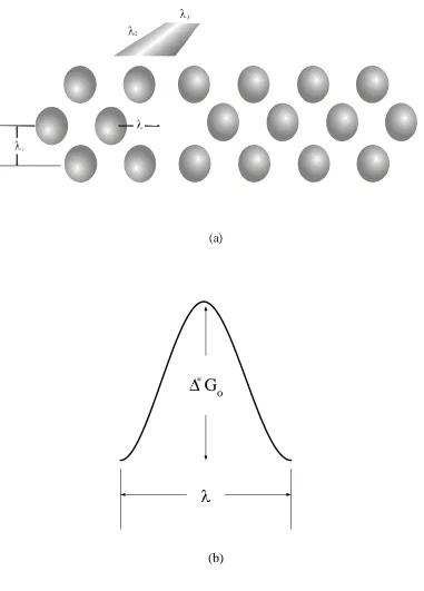
equilibrium position to another passing the energy barrier as shown in Figure 2.1a. Such

(35)

(a)

G

_o *

(b)

(36)

Figure 2.1b shows liquid molecules as described by Eyring (1936), in layers. A

distance λ1 between two adjacent layers experiencing shear forces and an average area

occupied by one molecule of λ2 λ3are assumed. Where λ2is the average distance between

neighboring molecules and λ3is the average distance between molecules normal to the

direction of motion.

A vacant site is required for the molecule to successively move from one position

to another. Eyring’s viscosity equation for liquids was derived as:

KT ΔG exp λ λ λ

hλ

η 0

2 3 2

1

(2.11)

where η is the absolute viscosity, h is Planck’s constant, K is Boltzman’s constant, and

λ is the average distance between equilibrium positions in the direction of motion.

Assuming that λ1= λ, and taking V0, the effective volume of a molecule, to be equal to λ1 λ2 λ3, equation (2.11) becomes

RT G Δ exp V

h

η 0

0

(2.12)

The above equation may be rewritten in the form of molar properties as

RT G Δ exp V hN η

m

(2.13)

where N is Avogadro’s number, Vm is the molar volume of the liquid, and

Δ*

(37)

2.4.1.1 McAllister’s model

A. Binary mixtures

McAllister (1960) developed his successful model, on the basis of Eyring’s

absolute rate theory, in terms of the kinematic viscosity of binary liquid mixtures as

follows:

RT G Δ exp M

hN ν

avg

(2.14)

where

i i i avg xM

M (2.15)

where the subscript i denotes component type 1 or 2, x is the mole fraction and M is the

molecular weight.

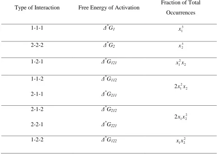
In a binary mixture of molecules of the type 1 and 2, McAllister assumed that

different possible types of interactions may occur in a solution with respect to the

molecule movement. McAllister (1960) assumed a three-body collision (or interaction).

Figure 2.2 depicts the different types of molecular interactions in a binary mixture

(occurs in one plane) and Table 2.1 shows the different types of molecular interactions

along with their corresponding free energies of activation and their fraction of total

(38)

(a) (b) (c) (d)

(e) _(f) (g) (h)

(39)

Table 2.1: Different Types of interactions in a binary mixture of molecules 1 and 2, their corresponding free energy of activation and their total of fractional occurrences (Three-Body Interaction Model)

Type of Interaction Free Energy of Activation Fraction of Total Occurrences

1-1-1 Δ*G1 x₁3

2-2-2 Δ*G2 x23

1-2-1 Δ*G121 x₁2x₂

1-1-2 Δ*G112

2 2 1 2x x

2-1-1 Δ*G211

2-1-2 Δ*G212

2 2 1 2x x

2-2-1 Δ*G221

(40)

According to McAllister (1960), the free energy of activation of the mixture is given by, 2 3 2 122 2 2 1 212 2 2 1 112 2 2 1 121 2 2 1 1 3 1 2 2 G x G x x G x x G x x G x x G x G (2.16)

Many assumptions were made by McAllister in order to derive his cubic equation.

These were,

(i) All types of interactions are only three bodied and are taking place in one

plane.

(ii) The ratio between the radii of the two types of molecules is taken arbitrarily to be 1.5; otherwise different additional interactions have to be considered (a

four-body interaction model).

(iii) The free energies of activation are additive, and the probability of

interaction is proportional to the mole fractions of the molecules involved.

(iv) Due to the difficulty in differentiating between Δ*G121 and Δ*G112 and similar

terms, it was assumed that

12 112

121 G G

G (2.17)

G212 G122 G21 (2.18)

On the basis of the above assumptions, equation (2.16) may be rewritten as

2 3 2 21 2 2 1 12 2 2 1 1 3

1 G 3x x G 3x x G x G

x

(41)

Applying equation (2.14) to each type of interaction involved in the mixture, i.e.

one can re-write an equation for the kinematic viscosity of the pure component 1 as

follows: RT G exp M hN 1 1

1 (2.20)

Similarly, for component 2

RT G exp M hN 2 2

2 (2.21)

For interactions of types 12 and 21,

RT G exp M hN 12 12

12 (2.22)

and RT G exp M hN 21 21

21 (2.23)

one also has the following relationship:

3

2 ₁ ₂

12

M M

M (2.24)

similarly,

3

2 ₂ ₁

21

M M

M (2.25)

3

2 ₁₁₂ ₁₂₁

12

G G

(42)

and

3

2 ₁₂₂ ₂₁₂

21

G G

G (2.27)

Substituting equation (2.19) into equation (2.14) one obtains:

RT G x G x x G x x G x exp M hN ave 2 3 2 21 2 2 1 12 2 2 1 1 3

1 3 3

(2.28)

Taking the logarithms of equations (2.20) through (2.23) and combining them in

order to eliminate the free energies, then substitute all of that along with equations (2.15),

(2.24), and (2.25) with some mathematical manipulations, one can obtain the final form

of the McAllister three-body model for binary mixtures as follows:

1 2 3 2 1 2 2 2 1 2 2 1 1 2 2 2 3 2 21 2 2 1 12 2 2 1 1 3 1 3 2 1 3 2 3 3 3 M / M n x M / M n x 3x M / M n x M M x x n -n x n x x n x x n x n 1 1          (2.29)

Equation (2.29) is a cubic equation which can have a maximum, a minimum,

neither or both for ν as a function of x. It should also be noted that the equation has only

two adjustable parameters; viz., ν12 and ν21 which can be determined by fitting the

(43)

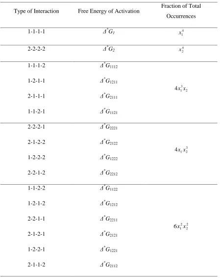
McAllister (1960) suggested a four-body interaction model to be applied for the

case of mixtures having large differences in their molecular size. McAllister followed a

similar procedure to that he had followed in deriving his three-body interaction model.

The final form of his “quartic equation” is as follows:

4 3 1 4 2 1 4 3 4 4 6 4 1 2 3 2 1 1 2 2 2 1 2 2 3 1 1 2 2 2221 3 2 1 1122 2 2 2 1 1112 2 3 1 1 4 1 M / M n x x M / M n x 6x M / M n x x M M x x n -n x n x x n x x n x x n x n 2 1 1 2 4 2           (2.30)

Table 2.2 shows the different types of interactions involved along with their

corresponding free energies and fractional occurrences.

The above equation, equation (2.30), contains three adjustable parameters;

namely, ν1112, ν1122, and ν2221 which again have to be determined from

viscosity-composition data.

The presence of the adjustable parameters in both the three-body and the

four-body models limits the use of the McAllister model because of the need for costly and

time consuming viscosity-composition data to determine the values of these parameters.

It should be pointed out here that the McAllister adjustable parameters are highly

temperature dependent which, again, is considered a major draw back of his models.

(44)

Table 2.2: Different Types of interactions in a binary mixture of molecules 1 and 2, their corresponding free energy of activation and their total of fractional occurrences (Four-Body Interaction Model)

Type of Interaction Free Energy of Activation Fraction of Total Occurrences

1-1-1-1 Δ*G1 x₁4

2-2-2-2 Δ*G2 x24

1-1-1-2 Δ*G1112

2 3 1 4x x

1-2-1-1 Δ*G1211

2-1-1-1 Δ*G2111

1-1-2-1 Δ*G1121

2-2-2-1 Δ*G2221

3 2 1 4x x

2-1-2-2 Δ*G2122

1-2-2-2 Δ*G1222

2-2-1-2 Δ*G2212

1-1-2-2 Δ*G1122

2 2 2 1 6x x

1-2-1-2 Δ*G1212

2-2-1-1 Δ*G2211

2-1-2-1 Δ*G2121

1-2-2-1 Δ*G1221

(45)

2.4.1.2 The Asfour et al (1991) technique

Realizing the importance of the McAllister model, Asfour et al. (1991) proposed

their technique which converts the McAllister model from a correlative model into a

predictive model. This was achieved by providing means for predicting the values of the

adjustable parameters from pure component and molecular properties. This obviously

eliminates the need for costly and time consuming experimental data.

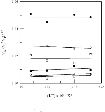
Asfour et al. (1991) successfully applied their technique to n-alkane mixtures.

They employed kinematic viscosity-composition data reported by Cooper (1988) and Wu

(1992). They plotted the lumped parameter ₁_/₃

2 2 1

12

versus the inverse of the absolute

temperature, (1/T). From the plot shown in Figure 2.3, horizontal straight lines were

obtained which confirmed that the lumped parameter is independent of temperature.

Asfour et al. (1991) plotted the lumped parameter against a fraction of the number of

carbon atoms of the n-alkanes constituting a binary system as shown in Figure 2.4. A

straight line relationship resulted. They suggested the following equation:

3 / 1 2 2 1

2 1 2 3

/ 1 2 2 1

12

044 . 0 1

N N

(2.31)

where N1 and N2 are the numbers of carbon atoms per molecule of components 1 and 2,

respectively.

Equation (2.31) permits the calculation of the value of the McAllister parameter,

ν12, by knowing the pure component kinematic viscosities and the number of carbon

(46)

Figure 2.3: Lumped Parameters, ₁_/₃

2 2 1

12

, Variation With (1/T) or n-alkane Systems

(47)

Figure 2.4: Lumped Parameter Variations, ₁_/₃

2 2 1

12

, with ₁_/₃

2 2 1

2 1 2

N N

For n-

(48)

the calculation of the second interaction parameter, ν21: 3 / 1 1 2 12

21 (2.32)

The above equation allows the calculation of the McAllister parameter, ν21, from the

value of ν12 obtained earlier from equation (2.31). Their results showed an absolute

average deviation in the range of 0.02 % to 1 % in predicting the kinematic viscosities of

binary n-alkane mixtures using the above technique compared to those calculated by the

correlative McAllister model.

As stated earlier by McAllister (1960), one should apply the four-body collision

model if the ratio between the molecular radii of the molecules in a binary mixture

exceeded 1.5. On that basis, Asfour et al. (1991) suggested a technique analogous to the

one reported for three-body interaction model to calculate the McAllister three adjustable

parameters mentioned earlier as follows:

4 / 1 2 2 2 1 2 1 2 4 / 1 2 2 2 1 1122 03 . 0 1 N N N N (2.33) 4 / 1 2 1 1122

1112 (2.34)

4 / 1 1 2 1122

(49)

Again, experimental data different than those used in developing the above

equations were used to validate the Asfour et al. (1991) proposed technique. The results

showed good agreement with published experimental data.

Nhaesi and Asfour (1998) extended the Asfour et al. (1991) technique to regular

binary mixtures. As a substitute for the number of carbon atoms in n-alkanes, they

suggested the use of the effective carbon number (ECN) concept in case of regular

systems. Nhaesi and Asfour (1998) reported a semi-log plot of the kinematic viscosities

of pure n-alkanes (C5-C18) measured at 308.15 K versus the number of carbon atoms in

each molecule. The straight line relation obtained is shown in Figure 2.5 which is

represented by the following equation

) 193 . 0 943 . 1 ECN n

 (2.36)

where, ν is the kinematic viscosity of the pure component at 308.15 K in cSt. Nhaesi

(1998) has reported values of the ECNs of some compounds calculated with the help of

equation (2.36).

The reported ECN values enabled Nhaesi and Asfour (1998) to develop a

technique for regular binary systems similar to equation (2.31) reported earlier for n

-alkane systems. The first binary adjustable parameter, ν12, for the case of regular

compounds may be calculated from

3 / 1 2 2 1 2 1 2 3 / 1 2 2 1 12 0715 . 0 8735 . 0 ECN ECN ECN ECN (2.37)

(50)

(51)

B. Ternary systems

Chandramouli and Laddha (1963) and Kalidas and Ladhha (1964) extended the

McAllister three-body model to ternary mixtures. Figure 2.6 represents the different types

of molecular interactions accompanied with the assumption of a three-body interaction

model. They obtained the following equation:

3 3 2 3 3 2 3 3 2 3 3 2 3 3 2 3 3 2 3 6 3 3 3 3 3 3 2 1 3 2 2 3 2 2 3 1 3 1 2 3 3 2 3 2 2 1 2 1 2 2 3 1 3 2 1 2 1 2 2 1 3 3 3 2 3 2 1 3 1 3 3 2 2 1 123 3 2 1 32 2 2 3 31 1 2 3 23 3 2 2 21 1 2 2 13 3 2 1 3 3 3 1 3 1 M M M n x x 6x M M n x x M M n x x M M n x x M M n x x M M n x x M M n x x nM x nM x nM x M x M x M x n n x x x n x x n x x n x x n x x 3 n x x n x x n x n x n x n 1 1 12 2 2 1 2 3 2                       (2.38)

Again, Nhaesi and Asfour (2000b) followed the same procedure described in the

previous section to calculate the McAllister’s adjustable parameters. They plotted the

dimensionless lumped parameter, ν123/(ν1 ν2 ν3)1/3 against 1/T, they obtained horizontal

(52)

(53)

straight line was obtained when they plotted ν123/(ν1 ν2 ν3)1/3 versus (N3-N1)2/N2 , where N1, N2, and N3 are the carbon numbers of components 1, 2, and 3, respectively.

Using the least-square technique they were able to get the equation of the straight

line as follows:

2 2 1 3 3 1 3 2 1 123 0313 0 9637 0 N N N . .

/ (2.39)

The above equation can be used to predict the ternary interaction parameter if the

kinematic viscosities of pure components and their number of carbon atoms are known.

In case of regular solutions the numbers of carbon atoms in equation (2.39) are replaced

by the effective carbon numbers.

C. Multi-component systems

Dizechi and Marschall (1982) introduced the first modification to the generalized

McAllister three-body equation. Their modified equation included two constants; C and Z

suggested earlier by Goletz and Tassios (1977) to account for the dependence of the

adjustable parameters on temperature. They suggested the following equation

(54)

where

n

i i i avg x M

M (2.41)

3

/ M 2M

M_ij _i _j (2.42)

3

/ M M M

M_ijk _i _j _k (2.43)

i , b

i Zt

C 239 (2.44)

n

i i i avg xC

C (2.45)

3

/ C 2C

C_ij _i _j (2.46)

3

/ C C C

C_ijk _i _j _k (2.47)

Dizechi (1980) reported in a study an optimizing technique for the determination

of the value of Z. He found that Z is a weak function of temperature therefore, only one

(55)

Dizechi and Marschall (1982) tested their model using data on eight binary and

four ternary polar liquid mixtures at various temperatures. The results of the comparison

between their model and the original McAllister equation showed improvements in the

prediction of viscosity of the mixtures.

Soliman (1987) continued the earlier work of Dizechi and Marschall (1982) and

attempted to reduce the number of adjustable parameters and to improve the capabilities

of the McAllister equation. He made some modifications to the original McAllister

equation and introduced only one constant, B, as follows:

2 -n 1 i 1 -n 1 i j n 2 j k ijk k j i j i j i j i ij 1 -n 1 i n 1 i j j i 1 -n 1 i n 1 i j ij j i n 1 i i 3 i m n x x x 6 x x M M x x B x x n x x n x n



2 3 3 (2.48)

For the above two modifications, equations (2.40) and (2.48), all the adjustable

parameters and the constants are to be determined from fitting experimental viscosity

data using the least square technique.

Soliman and Marschall (1990) reported a comparison on eight binary, five

ternary, and one quaternary liquid mixture containing strongly polar liquids including

water. As a result of the comparison made in their study amongest the three models, the

original McAllister equation, equation (2.40), and equation (2.48), Soliman’s (1987)

(56)

Although the two previous modifications to the original McAllister equation for

multi-component liquid mixtures showed a remarkable improvement in the liquid mixture

viscosities, it still did not change the correlative nature of the original McAllister model.

Extensivee databases are needed to calculate the introduced constants besides the

adjustable parameters which are not readily available in all cases.

Nhaesi and Asfour (2000b) were able to develop a generalized form of

McAllister’s three-body equation for multi-component liquid mixtures.

They suggested that the activation energy for n-component liquid systems can be

represented by the following general equation:

n 1 i n 1 j n 1 k ijk k j i ij j n 1 i n 1 j 2 i i n 1 i 3 i m G x x x 6 G x 3 G x

G x

(2.49)

Taking into consideration that the free energies of activation for kinematic

viscosities are additive. They also assumed the following:

ij iij

iji G G

G (2.50)

ji ijj

jij G G

G (2.51)

The kinematic viscosities for pure component, binary interaction, ternary

interaction, or a mixture may be expressed in the form of Arrhenius-type equation as

Viscosities and Densities of Some Multi-Component Regular Liquid Solutions at Different Temperature Levels

Scholarship at UWindsor

Scholarship at UWindsor

Viscosities and Densities of Some Multi-Component Regular

Viscosities and Densities of Some Multi-Component Regular

Liquid Solutions at Different Temperature Levels

Liquid Solutions at Different Temperature Levels

Liquid Solutions at Different Temperature Levels

By

Hanan El-Sayed Moussa El-Sayed

A Dissertation

Submitted to the Faculty of Graduate Studies

through the Environmental Engineering Program

in Partial Fulfillment of the Requirements for

the Degree of Doctor of Philosophy at the

University of Windsor

Windsor, Ontario, Canada

2009

Author’s Declaration of Originality

ABSTRACT

DEDICATION

ACKNOWLEDGEMENTS

TABLE OF CONTENTS

LIST OF TABLES

LIST OF FIGURES

CHAPTER 1

INTRODUCTION

CHAPTER 2

LITERATURE SURVEY















G









_

_

_