University of Windsor University of Windsor
Scholarship at UWindsor
Scholarship at UWindsor
Electronic Theses and Dissertations Theses, Dissertations, and Major Papers
2-18-2016
Modeling and Performance Analysis of Manufacturing Systems
Modeling and Performance Analysis of Manufacturing Systems
Using Max-Plus Algebra
Using Max-Plus Algebra
Abdulrahman Saad Salah-Eldin Seleim University of Windsor
Follow this and additional works at: https://scholar.uwindsor.ca/etd
Recommended Citation Recommended Citation
Seleim, Abdulrahman Saad Salah-Eldin, "Modeling and Performance Analysis of Manufacturing Systems Using Max-Plus Algebra" (2016). Electronic Theses and Dissertations. 5665.
https://scholar.uwindsor.ca/etd/5665
This online database contains the full-text of PhD dissertations and Masters’ theses of University of Windsor students from 1954 forward. These documents are made available for personal study and research purposes only, in accordance with the Canadian Copyright Act and the Creative Commons license—CC BY-NC-ND (Attribution, Non-Commercial, No Derivative Works). Under this license, works must always be attributed to the copyright holder (original author), cannot be used for any commercial purposes, and may not be altered. Any other use would require the permission of the copyright holder. Students may inquire about withdrawing their dissertation and/or thesis from this database. For additional inquiries, please contact the repository administrator via email
Modeling and Performance Analysis of Manufacturing Systems Using Max-Plus Algebra
By
Abdulrahman Seleim
A Dissertation
Submitted to the Faculty of Graduate Studies
through the Department of Industrial and Manufacturing Systems Engineering
in Partial Fulfillment of the Requirements for
the Degree of Doctor of Philosophy
at the University of Windsor
Windsor, Ontario, Canada
2016
Modeling and Performance Analysis of Manufacturing Systems Using Max-Plus Algebra
by
Abdulrahman Seleim
APPROVED BY:
______________________________________________
Dr. Pedro Cunha, External Examiner
Escola Superior de Tecnologia/Instituto Politécnico de Setubal, Portugal
______________________________________________
Dr. Xiaobu Yuan
School of Computer Science
______________________________________________
Dr. Zbignew Pasek
Industrial and Manufacturing Systems Engineering
______________________________________________
Dr. Fazle Baki
Industrial and Manufacturing Systems Engineering
______________________________________________
Dr. Hoda ElMaraghy, Advisor
Industrial and Manufacturing Systems Engineering
iii
DECLARATION OF CO-AUTHORSHIP / PREVIOUS PUBLICATION
I. Co-Authorship Declaration
I hereby declare that this thesis incorporates material that is result of joint research of the author and his supervisor Prof. Hoda ElMaraghy. This joint research has been published / submitted to various Journals that are listed below.
I am aware of the University of Windsor Senate Policy on Authorship and I certify that I have properly acknowledged the contribution of other researchers to my thesis, and have obtained written permission from Prof. Hoda ElMaraghy to include that material(s) in my thesis. I certify that, with the above qualification, this thesis, and the research to which it refers, is the product of my own work.
II. Declaration of Previous Publication
This thesis includes 4 original papers that have been previously published / submitted for publication in peer reviewed journals and conferences as follows:
Thesis Chapter
Publication title/full citation Publication Status 3 Seleim, A. and H. ElMaraghy (2015). "Generating max-plus equations for
efficient analysis of manufacturing flow lines." Journal of Manufacturing Systems 37: 426-436.
Journal (Published)
4 Seleim, A. and H. ElMaraghy (2014). "Parametric analysis of Mixed-Model Assembly Lines using max-plus algebra." CIRP Journal of Manufacturing Science and Technology 7(4): 305-314.
Journal (Published)
3 Seleim, A., ElMaraghy, H., (2014). "Max-Plus Modeling of Manufacturing Flow Lines", Proceedings of the 47th CIRP Conference on Manufacturing Systems (CMS2014), Windsor, ON , Canada, Procedia CIRP, Vol. 17, pp. 302-307.
Conference Proceeding
5 Seleim, A., ElMaraghy, H., (2013). "Transient Analysis of a Re-entrant Manufacturing System", 5th International Conference on Changeable, Agile, Reconfigurable and Virtual Production (CARV2013), Munich, Germany, pp. 261-266.
Conference Proceeding
I certify that I have obtained a written permission from the copyright owner(s) to include the above published material(s) in my thesis. I certify that the above material describes work completed during my registration as graduate student at the University of Windsor.
iv acknowledged in accordance with the standard referencing practices. Furthermore, to the extent that I have included copyrighted material that surpasses the bounds of fair dealing within the meaning of the Canada Copyright Act, I certify that I have obtained a written permission from the copyright owner(s) to include such material(s) in my thesis.
v
ABSTRACT
In response to increased competition, manufacturing systems are becoming more complex in order to provide the flexibility and responsiveness required by the market. The increased complexity requires decision support tools that can provide insight into the effect of system changes on performance in an efficient and timely manner.
Max-Plus algebra is a mathematical tool that can model manufacturing systems in linear equations similar to state-space equations used to model physical systems. These equations can be used in providing insight into the performance of systems that would otherwise require numerous time consuming simulations.
This research tackles two challenges that currently hinder the applicability of the use of max-plus algebra in industry. The first problem is the difficulty of deriving the max-plus equations that model complex manufacturing systems. That challenge was overcome through developing a method for automatically generating the max-plus equations for manufacturing systems and presenting them in a form that allows analyzing and comparing any number of possible line configurations in an efficient manner; as well as giving insights into the effects of changing system parameters such as the effects of adding buffers to the system or changing buffers sizes on various system performance measures. The developed equations can also be used in the operation phase to analyze possible line improvements and line reconfigurations due to product changes. The second challenge is the absence of max-plus models for special types of manufacturing systems. For this, max-plus models were developed for the first time for modeling mixed model assembly lines (MMALs) and re-entrant manufacturing systems.
vi
DEDICATION
vii
ACKNOWLEDGEMENTS
Before all, praise goes to God for giving me the strength and knowledge to complete this work. The completion of this dissertation would not have been possible without the support and help of many people, to whom I would like to express my gratitude. On top of the list comes Prof. Hoda ElMaraghy, my supervisor, who provided me with continuous and invaluable support, guidance, and mentorship. I would also like to express my appreciation to the PhD committee members: Dr. Pedro Cuhna, Dr. Xiaobu Yuan, Dr. Zbignew Pasek, andDr. Fazle Baki , for their valuable comments and suggestions which vastly improved the quality of the dissertation. Special thanks also go to my colleagues and mentors at the Intelligent Manufacturing Systems Centre (IMSC) at the University of Windsor, Prof. Waguih ElMaraghy, Dr. Ahmed Deif, Dr. Ayman Youssef, Dr. Tarek AlGeddawy, Dr. Sameh Samy, Dr. Mohammed Hanafy, Ahmed Adawy, Dr. Mohamed Kashkoush, Mohamed Abbas, Javad Navaei and Kourosh Khedri, with whom I had numerous comments, suggestions, and stimulating discussions.
viii
TABLE OF CONTENTS
DECLARATION OF CO-AUTHORSHIP / PREVIOUS PUBLICATION ... iii
ABSTRACT ...v
DEDICATION ... vi
ACKNOWLEDGEMENTS ... vii
LIST OF TABLES ...x
LIST OF FIGURES ... xi
Chapter 1: INTRODUCTION...1
1.1. Motivation ... 1
1.2. Scope ... 2
1.3. Thesis Statement ... 3
1.4. Max-Plus Algebra ... 3
1.5. Dissertation Overview ... 4
Chapter 2: BASICS OF MAX-PLUS ALGEBRA ...6
2.1. Max-plus Algebra Basics ... 6
2.2. Example of Modeling a Manufacturing System ... 9
2.3. Coding Max-plus Algebra in Wolfram Mathematica ... 12
Chapter 3: MAX-PLUS MODELING OF MANFUFACTURING FLOW LINES ...13
3.1. Introduction ... 13
3.2. Related Research ... 13
3.3. Flow Lines Modeling ... 14
3.4. Case Study and Analysis ... 27
3.5. Discussion and Conclusions ... 33
Chapter 4: MAX-PLUS MODELING OF MIXED-MODEL ASSEMBLY LINES ...35
4.1. Introduction ... 35
4.2. Modeling MMALS ... 37
4.3. Numerical Examples ... 44
4.4. Industrial Case Study: MMAL of Auto Car Seats ... 53
ix
Chapter 5: MAX-PLUS MODELING OF RE-ENTRANT MANUFACTURING
SYSTEMS...60
5.1. Introduction ... 60
5.2. Literature Review... 61
5.3. Re-Entrant Manufacturing System Description ... 64
5.4. System Modeling ... 65
5.5. Max-Plus System Model Analysis ... 67
5.6. Discussion and Conclusions ... 75
Chapter 6: DISCUSSION AND CONCLUSIONS...77
6.1. Discussion and Overview ... 77
6.2. Research Significance ... 79
6.3. Research Contributions and Novelty ... 80
6.4. Future Work ... 80
REFERENCES ...82
APPENDIX A ...87
APPENDIX B ...88
APPENDIX C ...90
APPENDIX D ...92
x
LIST OF TABLES
Table 1-1 Summary of Literature Review ... 5
Table 3-1 Assembly processes and required processing times for stations in Figure 3.11 (b). .... 30
Table 3-2 Starting times for 10 jobs for configuration 1. ... 31
Table 3-3 Summary of results from Figure 3.13 ... 33
Table 4-1 Assembly times for each model in each station... 45
Table 4-2 Optimal sequence for system parameters in Table 4.1 as obtained from (Bard, Dar-El et al. 1992). ... 45
Table 4-3 Sequences to be compared. ... 46
Table 4-4 Required time in seconds for each seat configuration at each station. ... 55
Table 4-5 Optimal sequences for different 𝒕𝟏, 𝟏... 56
xi
LIST OF FIGURES
Figure 1.1 Classification of DEDS modeling tools ... 2
Figure 2.1 A simple 3 machine manufacturing system. ... 10
Figure 3.1 Flow line with n serial stations ... 15
Figure 3.2 Flow line with n merging lines ... 16
Figure 3.3 A three stage flow line with n parallel identical stations in the second stage. ... 19
Figure 3.4 Flow line with parallel identical stations in several stages ... 20
Figure 3.5 Flow line with 4 serial stations and 3 finite buffers... 22
Figure 3.6 General flow line. (a) Line with parallel identical machines and buffers. (b) Line after simplification. ... 24
Figure 3.7 A general flow line and its corresponding adjacency matrix... 24
Figure 3.8 Adjacency matrix and its corresponding flow line diagram after re-arranging the rows and columns of the matrix ... 25
Figure 3.9 Automated Valve assembly line (Delta-Tech). ... 27
Figure 3.10 Back flushing control valve components (Dorot (2001)). ... 29
Figure 3.11 Assembly sequence tree (Kashkoush and ElMaraghy 2014) (a) and three possible corresponding assembly line configurations (b). ... 29
Figure 3.12 The effect of buffers size on total line idle time for the three line configurations given in figure 3.10. ... 32
Figure 3.13 Total line idle time for configuration 3 as a function of the processing time of station E*. ... 32
Figure 4.1 Worker movement in a continuous transport MMAL with closed stations. ... 40
Figure 4.2 Worker movement in a continuous transport MMAL with open stations. ... 40
Figure 4.3 Job starting scenarios for workers in a closed station MMAL. ... 41
Figure 4.4 Total line length as a function of assembly times 𝒕𝟏, 𝟐, 𝒕𝟐, 𝟐, 𝒕𝟑, 𝟏 and 𝒕𝟒, 𝟐 for closed stations MMAL. ... 47
Figure 4.5 Total line length as a function of assembly times 𝒕𝟏, 𝟐, 𝒕𝟐, 𝟐, 𝒕𝟑, 𝟏 and 𝒕𝟒, 𝟐 for open stations MMAL. ... 48
Figure 4.6 Starting position of each job on the line for closed stations with 𝒍𝒕= 4 (a) and 𝑙=8 (b). ... 49
Figure 4.7 Starting position of each job on the line for open stations with 𝒍𝒕= 4 (a) and 𝒍𝒕=8 (b). ... 50
Figure 4.8 Total idle and line length as a function of 𝒍𝒕 for closed stations MMAL. ... 51
Figure 4.9 Total idle and line length as a function of 𝒍𝒕 for open stations MMAL. ... 51
Figure 4.10 Total throughput time as a function of 𝒍𝒕 for closed stations MMAL. ... 52
Figure 4.11 Total throughput time as a function of 𝒍𝒕 for open stations MMAL. ... 53
Figure 4.12 Assembly line stations for front seat. ... 54
Figure 4.13 Main seat components. ... 54
Figure 4.14 Total line length as a function of assembly time 𝒕𝟏, 𝟏 ... 57
Figure 4.15 Total line idle time as a function of assembly time 𝒕𝟏, 𝟏 ... 57
xii Figure 5.1 Examples of simple re-entrant manufacturing systems. (a) Part of layout of fuel
1
CHAPTER 1:
INTRODUCTION
1.1.
Motivation
In today’s highly competitive market, it is not enough to produce products with excellent quality and low price. Under fierce competition, manufacturers are required to introduce a wide variety of products and produce them in the right quantity and at the right time. Under these circumstances, decision makers require good supporting tools that they can use to understand which parameters affect their production system as well as effect of each of these parameters on the overall performance.
Manufacturing systems can be classified under the category of Discrete Event Dynamic Systems (DEDSs) which also includes computer systems, traffic systems, and communication systems. What characterizes these systems is that their state changes not with time, but with certain events and the change from one state to another takes place instantaneously. For manufacturing systems, such events can be the arrival of a work piece, the breakdown of a machine, etc. These systems are structurally different from natural physical dynamic systems that are governed by differential equations. The behavior and natural physical systems can be accurately monitored, explained, predicted and controlled by the use of differential equations; on the other hand, for DEDSs such a robust and powerful mathematical tool does not exist yet (Cassandras and Lafortune 2007)(Cassandras and Lafortune 2007).
2 Figure 1.1 Classification of DEDS modeling tools
Max-plus algebra is an algebraic mathematical formulation that can be used to model manufacturing systems by linear state-space like equations. By modeling manufacturing systems using max-plus algebra, one can arrive at mathematical equations that can be used in the analysis and control of manufacturing systems. The use of max-plus algebra in modeling and analysis of manufacturing systems started in the nineteen eighties; however its use both commercially and academically has been limited. This is mainly because using the tool requires special mathematical background and because there are no user-friendly tools that facilitate the use of max-plus algebra in modeling and analysis of systems.
1.2.
Scope
3 The first of these tools is a method for the automatic generation of max-plus equations for manufacturing flow lines. The method can be used to model lines with finite buffers and parallel identical stations and produces equations that can be used in parametric analysis.
The second tool is a novel approach in modeling mix-model assembly lines with max-plus algebra. The developed equations can then be used to compare given sequences of demand mix over a range of processing times of assembly tasks as well as analyze different line performance measures while considering one of the line parameters as a variable. Hence, the effect of changes in any of the system parameters on the optimality of a given sequence of demand mix and on the line performance can be assessed.
The third tool is method for modeling re-entrant manufacturing systems which are used widely in semiconductor manufacturing and paint shops. Using the developed equations, complex behavior especially in the transient phase can be detected and avoided.
It should be noted that the manufacturing systems modeled by max-plus algebra in this thesis do not cover all types of manufacturing systems. However, they represent structurally different types of systems and thus prove in principle that this tool is capable of modeling and providing useful analysis to a wide range of manufacturing systems.
1.3.
Thesis Statement
The use of max-plus algebra in modeling and analysis of manufacturing systems can provide insights and information about the systems performance that cannot be otherwise efficiently obtained with available modeling tools
1.4.
Max-Plus Algebra
4 Research related to max-plus algebra can be classified into two different categories. The first is research in developing the tool itself and increasing its appeal to potential users. Work in this category includes direct generation of max-plus equations for flow shop systems (Doustmohammadi and Kamen 1995; Seleim and ElMaraghy 2015), extending max-plus algebra to stochastic systems (Jean-Marie and Olsder 1996), introducing buffer and capacity constraints to the max-plus representation of manufacturing systems (Goto, Shoji et al. 2007), and introducing a block diagram based representation of manufacturing systems using max-plus algebra (Imaev and Judd 2008; Imaev and Judd 2009).
The second category of research related to max-plus algebra is concerned with applications of the tool. These include manufacturing systems modeling (Ren, Xu et al. 2007; Imaev and Judd 2008; Imaev and Judd 2009; Seleim and ElMaraghy 2014), performance evaluation (Cohen, Dubois et al. 1985; Amari, Demongodin et al. 2005; Reddy, Janardhana et al. 2009; Morrison 2010; Park and Morrison 2010; Boukra, Lahaye et al. 2013; Seleim and ElMaraghy 2014; Singh and Judd 2014), performance optimization (Di Febbraro, Minciardi et al. 1994), scheduling (Lee 2000; Goto, Hasegawa et al. 2007; Tanaka, Masuda et al. 2009; Houssin 2011) model predictive control (De Schutter and Van Den Boom 2001; van den Boom and De Schutter 2006; Goto 2013).
1.5.
Dissertation Overview
5
Table 1-1 Summary of Literature Review
Tool Development Applications
Equations generation (Doustmohammadi and Kamen 1995; Seleim
and ElMaraghy 2015)
Modeling manufacturing systems
(Ren, Xu et al. 2007;
Imaev and Judd 2008;
Imaev and Judd 2009;
Seleim and ElMaraghy
2014)
Modeling Stochastic Systems
(Jean-Marie and Olsder
1996)
Performance evaluation
(Cohen, Dubois et al.
1985; Amari,
Demongodin et al.
2005; Reddy,
Janardhana et al. 2009;
Morrison 2010; Park
and Morrison 2010;
Boukra, Lahaye et al.
2013; Singh and Judd
2014)
Buffer and capacity constraints
(Goto, Shoji et al.
2007)
Performance optimization
(Di Febbraro, Minciardi
et al. 1994)
Block diagram
representation
(Imaev and Judd 2008;
Imaev and Judd 2009)
Scheduling (Lee 2000; Goto,
Hasegawa et al. 2007;
Tanaka, Masuda et al.
2009; Houssin 2011)
Control (De Schutter and Van
Den Boom 2001; van
den Boom and De
Schutter 2006; Houssin,
Lahaye et al. 2007;
Goto 2013)
6
CHAPTER 2:
BASICS OF MAX-PLUS ALGEBRA
Max-plus algebra is one of many algebraic structures called semirings or dioids that are studied by mathematicians. The most famous of these semirings are the max-plus algebra, min-plus algebra, and the min-max algebra. These algebraic tools have been studied by mathematicians for many years and used in areas of optimization and algebraic geometry, but the first use of these tools in modeling discrete event systems was in 1985 by Cohen et al.(Cohen, Dubois et al. 1985). In their paper, Cohen et al. indicated that deterministic, discrete event systems can be represented in a linear state-space representation when modeled by these algebraic structures. Following that paper, max-plus algebra started to be used in modeling, control, and performance analysis of discrete event systems (Cohen, Gaubert et al. 1999).
In this chapter an introduction to the basic concepts and tools of the Max-Plus algebra is first presented then used to model a simple manufacturing system consisting of three machines. A more detailed presentation of max-plus algebra with in depth mathematical analysis and proofs can be found in (Baccelli, Cohen et al. 1992) and (Heidergott, Olsder et al. 2006).
2.1.
Max-plus Algebra Basics
Max-Plus algebra is defined over ℛ𝑚𝑎𝑥= {ℛ ∪ −∞} where ℛ is the set of real numbers. The two main algebraic operations are maximization, denoted by the symbol ⊕, and addition, denoted by the symbol ⨂ where:
𝑎 ⊕ 𝑏 = 𝑚𝑎𝑥(𝑎, 𝑏) ∀ 𝑎, 𝑏 ∈ ℛ𝑚𝑎𝑥
𝑎 ⊗ 𝑏 = 𝑎 + 𝑏 ∀ 𝑎, 𝑏 ∈ ℛ𝑚𝑎𝑥
Define 𝜀 = −∞ and 𝑒 = 0. In max-plus algebra, 𝜀 is the null element of the operation ⊕ where
𝑎 ⊕ 𝜀 = 𝑚𝑎𝑥 (𝑎, −∞) = 𝑎 ∀ 𝑎 ∈ ℛ𝑚𝑎𝑥
and 𝑒 is the null element for the operation ⊗ where
7 Throughout the rest of this dissertation, ⊕ will be referred to as addition (or plus) and ⊗ will be referred to as multiplication. Similar to traditional algebra, both ⊕ and ⊗ are associative and commutative
𝑎 ⊗ 𝑏 = 𝑏 ⊗ 𝑎 ∀ 𝑎, 𝑏 ∈ ℛ𝑚𝑎𝑥
(𝑎 ⊗ 𝑏) ⊗ 𝑐 = 𝑎 ⊗ (𝑏 ⊗ 𝑐) ∀ 𝑎, 𝑏, 𝑐 ∈ ℛ𝑚𝑎𝑥
𝑎 ⊕ 𝑏 = 𝑏 ⊕ 𝑎 ∀ 𝑎, 𝑏 ∈ ℛ𝑚𝑎𝑥
(𝑎 ⊕ 𝑏) ⊕ 𝑐 = 𝑎 ⊕ (𝑏 ⊕ 𝑐) ∀ 𝑎, 𝑏, 𝑐 ∈ ℛ𝑚𝑎𝑥
and multiplication is left and right distributive over addition
𝑎 ⊗ (𝑏 ⊕ 𝑐) = (𝑎 ⊗ 𝑏) ⊕ (𝑎 ⊗ 𝑐) ∀ 𝑎, 𝑏, 𝑐 ∈ ℛ𝑚𝑎𝑥
(𝑎 ⊕ 𝑏) ⊗ 𝑐 = (𝑎 ⊗ 𝑐) ⊕ (𝑏 ⊗ 𝑐) ∀ 𝑎, 𝑏, 𝑐 ∈ ℛ𝑚𝑎𝑥
Similar to conventional algebra, max-plus algebra can be extended over matrices. Let 𝑨 and 𝑩 be two matrices with equal dimension, then
𝑨⨁𝑩 = 𝑪
where 𝑪𝑖𝑗= 𝑨𝑖𝑗⨁ 𝑩𝑖𝑗. If the number of columns of 𝑨 is equal to the number of rows of 𝑩 equal to 𝑛, then:
𝑨 ⊗ 𝑩 = 𝑪
where
𝑪𝑖𝑗=
𝑛 ⨁ 𝑘 = 1
𝑨𝑖𝑘⊗ 𝑩𝑘𝑗
where ⊕𝑘=1𝑛 𝒒 is maximization of all the elements of 𝒒 for 𝑘 = 1 to 𝑛.
If 𝑎 is a scalar and 𝑨 is a matrix, then 𝑎 ⊗ 𝐴 is equivalent to adding the value of 𝑎 to each element in the matrix 𝐴.
8
𝑨 = [3 2𝑒 𝜀 ] , 𝑩 = [𝑒 69 1] , 𝑪 = [7 9 𝜀2 𝑒 4] 𝑎𝑛𝑑 𝑫 = [1 5𝑒 𝜀
7 3
],
then:
4 ⊗ 𝑨 = [3 + 4 2 + 4𝑒 + 4 𝜀 + 4] = [7 64 𝜀]
𝑨 ⊕ 𝑩 = [3 ⊕ 𝑒 2 ⊕ 6𝑒 ⊕ 9 𝜀 ⊕ 1]= [3 69 1]
𝑨 ⊗ 𝑩 = [3 ⊗ 𝑒 ⊕ 2 ⊗ 9 3 ⊗ 6 ⊕ 2 ⊗ 1𝑒 ⊗ 𝑒 ⊕ 𝜀 ⊗ 9 𝑒 ⊗ 6 ⊕ 𝜀 ⊗ 1]= [11 9𝑒 6]
𝑪 ⊗ 𝑫 = [(2 ⊗ 1) ⊕ (𝑒 ⊗ 𝑒) ⊕ (4 ⊗ 7) (2 ⊗ 5) ⊕ (𝑒 ⊗ 𝜀) ⊕ (4 ⊗ 3)(7 ⊗ 1) ⊕ (9 ⊗ 𝑒) ⊕ (𝜀 ⊗ 7) (7 ⊗ 5) ⊕ (9 ⊗ 𝜀) ⊕ (𝜀 ⊗ 3)]
= [ 911 127]
𝑨 ⊗ 𝑨 = 𝑨𝟐= [3 ⊗ 3 ⊕ 2 ⊗ 𝑒 3 ⊗ 2 ⊕ 2 ⊗ 𝜀
𝑒 ⊗ 3 ⊕ 𝜀 ⊗ 𝑒 𝑒 ⊗ 2 ⊕ 𝜀 ⊗ 𝜀]= [6 53 2]
Through the rest of the dissertation, the ⊗ operator will be omitted whenever its use is obvious, thus 𝑎 ⊗ 𝑏 ⊕ 𝑐 ⊗ 𝑑 will be written as 𝑎𝑏 ⊕ 𝑐𝑑.
Theorem 2.1:
An equation is the general form:
𝑿 = 𝑨 𝑿 ⊕ 𝑩 𝑼 (2.1)
where 𝑿 is an 𝑛 × 1 vector of variables, 𝑼 is an 𝑚 × 1 vector of inputs, 𝑨 is an 𝑛 × 𝑛 square matrix and 𝑩 is an 𝑛 × 𝑚 matrix, has a solution :
𝑿 = 𝑨∗ 𝑩 𝑼 (2.2)
where 𝑨∗is defined as:
𝑨∗= 𝑒 ⊕ 𝑨 ⊕ 𝑨2⊕ … ⊕ 𝑨∞ (2.3)
9 If matrix 𝐀 is regarded as a directed graph and the each entry 𝐀𝑖,𝑗denote the weight of path from node i to j, then 𝐀n𝑖,𝑗 denotes the weights of paths with length n in the same graph. Therefore, for
𝐀∗to have a defined value, the weights of paths larger than a given z should equal to zero and thus we get 𝐀n= −∞ for 𝑛 > 𝑧 and equation (2.3) becomes:
𝑨∗= 𝑒 ⊕ 𝑨 ⊕ 𝑨2⊕ … ⊕ 𝑨𝑧 (2.4)
For an 𝑛 × 𝑛 matrix 𝑨, an 𝑛 × 1 vector 𝝂, and a scalar 𝜇, if
𝑨 ⊗ 𝝂 = 𝜇 ⊗ 𝝂 (2.5)
then 𝜇 is called the eigenvalue of 𝑨 and 𝝂 is its associated eigenvector. Assume, 𝑿 is a vector of variables defining a system such that:
𝑿𝒌+𝟏 = 𝑨 𝑿𝒌
then at steady state, the eigenvalue of 𝑨 is the average growth rate of 𝑋. The eigenvalues can be calculated using different numerical algorithms presented in (Heidergott, Olsder et al. 2006).
2.2.
Example of Modeling a Manufacturing System
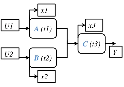
10
Figure 2.1 A simple 3 machine manufacturing system.
Considering station A, the time at which the station starts processing job k is the later of the two the two events: 1) required inputs for job k are available, which is equal to U1k, and 2) station A has finished processing the job k-1, which is equal to the time at which station A started processing the job k-1 plus the processing time on station A. In conventional algebra this can be written as:
𝑥1𝑘 = 𝑚𝑎𝑥 (𝑈1𝑘, 𝑥1𝑘−1+ 𝑡1) (2.6)
Similarly for station B, the time at which the station starts processing job k can be written as:
𝑥2𝑘 = 𝑚𝑎𝑥 (𝑈2𝑘, 𝑥2𝑘−1+ 𝑡2) (2.7)
For station C, processing the kth jobs can start at the latest of three events:
1) station A has finished processing the kth job, which is equal to 𝑥1𝑘+ 𝑡1,
2) station B has finished processing the kth job, which is equal to 𝑥2𝑘+ 𝑡2,
3) station C has finished processing the job k-1.
In conventional algebra this can be written as:
𝑥3𝑘 = 𝑚𝑎𝑥 (𝑥1𝑘+ 𝑡1, 𝑥2𝑘+ 𝑡2, 𝑥3𝑘−1+ 𝑡3) (2.8)
Equations (2.6-2.8) can be written in max-plus algebra as:
A
(t1)
C
(t3)
B
(t2)
U1
U2
Y
x1
x2
11
𝑥1𝑘 = 𝑈1𝑘⊕ 𝑡1 𝑥1𝑘−1 (2.9)
𝑥2𝑘 = 𝑈2𝑘⊕ 𝑡2 𝑥2𝑘−1 (2.10)
𝑥3𝑘 = 𝑡1𝑥1𝑘⊕ 𝑡2 𝑥2𝑘⊕ 𝑡3 𝑥3𝑘−1 (2.11)
The arrival time of the kth finished product is equal to the time it started processing on station C plus the processing time on station C, this can be written as:
𝒀𝑘 = 𝑡3 𝑥3𝑘 (2.12)
Equations (2.9-2.12) fully describe the simple manufacturing system in figure 2.1 and can be put in state-space vector form as:
𝑿𝑘 = 𝑨 𝑿𝑘⊕ 𝑩 𝑿𝑘−1⊕ 𝑫 𝑼𝑘 (2.13)
𝒀𝑘= 𝑪 𝑿𝑘 (2.14)
where: 𝑿𝑘 = [ 𝑥1 𝑥2 𝑥3 ] 𝑘
, 𝑼𝑘 = [𝑈1 𝑈2]
𝑘, 𝑨 = [ 𝜀 𝜀 𝑡1 𝜀 𝜀 𝑡2 𝜀 𝜀 𝜀] , 𝑩 = [ 𝑡1 𝜀 𝜀 𝜀 𝑡2 𝜀 𝜀 𝜀
𝑡3] , 𝑫 = [
𝑒 𝜀 𝜀 𝜀 𝑒 𝜀],
𝑪 = [𝜀 𝜀 𝑡3].
Notice that equation (2.13) is implicit in 𝐗k. According to theorem (2.1), the implicit equation (2.13) can be transformed into:
𝑿𝑘 = 𝑨̂ 𝑿𝑘−1⊕ 𝑩̂ 𝑼𝑘 (2.15)
where 𝑨̂ = 𝑨∗𝑩 , 𝑩̂ = 𝑨∗𝑫 and using equation (2.4)𝑨∗, 𝐀̂and 𝑩̂ can be calculated as:
𝑨∗= 𝑒 ⊕ 𝑨 ⊕ 𝑨𝟐= [𝑒𝜀 𝜀 𝜀 𝑒 𝜀 𝜀 𝜀 𝑒] ⊕ [ 𝜀 𝜀 𝑡1 𝜀 𝜀 𝑡2 𝜀 𝜀 𝜀] ⊕ [ 𝜀 𝜀 𝜀 𝜀 𝜀 𝜀 𝜀 𝜀 𝜀] = [ 𝑒 𝜀 𝑡1 𝜀 𝑒 𝑡2 𝜀 𝜀 𝑒],
𝑨̂ = 𝑨∗𝑩 = [𝑡1𝜀
𝑡1 𝜀 𝑡2 𝑡2 𝜀 𝜀
𝑡3], and 𝑩̂ = 𝑨
∗𝑫 = [𝑒𝜀
𝑡1 𝜀 𝑒
𝑡2].
12 can be determined. These equations can then be used in dynamic analysis of the system as well as in dynamic control as mentioned in section 1.4.
It should be noted, however, that the example presented above assumes infinite buffer capacity between stations A and B and station C. Accounting for finite buffers between stations will be considered in chapter 3 when considering the method to automatically generate the equations for manufacturing flow lines.
In the case when different products are processed on the same manufacturing system and different products have different processing times on each machine, equations (2.14) and (2.15) can still be used while changing the parameters t1, t2, and t3 into t1k, t2k
,
and t3k and accordingly the matricesA, B, and C will be changed to Ak, Bk, and Ck.
2.3.
Coding Max-plus Algebra in Wolfram Mathematica
13
CHAPTER 3:
MAX-PLUS MODELING OF
MANFUFACTURING FLOW LINES
3.1.
Introduction
Modeling simple manufacturing systems using max-plus equations is easy and intuitive; however, as the systems grow in size and/or have complicated structure, deriving the model equations becomes tedious, less intuitive and time consuming. In addition, deriving max-plus equations for manufacturing systems with finite buffers or parallel identical stations is not straight-forward or easy even for simple systems. The difficulty of deriving these equations limits the benefits of using max-plus algebra in modeling and controlling manufacturing systems especially when frequent changes in products or system configurations take place and the need for quickly assessing their effects and making decisions intensifies.
In this chapter, a method for automatic generation of the max-plus system equations for flow lines is presented. The method can generate the equations for lines with complicated structures regardless of their size and can model finite buffers and parallel identical stations. Flow lines studied in this chapter are assumed to have deterministic processing times and reliable stations. The first assumption is realistic for automated systems as well as semi-automated systems with palletized material handling where the process time variation is much less than the processing time and thus can be neglected. The second assumption is also realistic when studying the short-term system operation with the objective of understanding and optimizing the system behavior rather than studying the long-term operation with the objective of planning system capacity where machines breakdown would have an effect.
A review of related research is presented in section 3.2. Section 3.3 presents the method for generating the max-plus equations followed by a case study with an example of analysis in section 3.4, and finally section 3.5 presents the discussion and conclusions.
3.2.
Related Research
14 parallel machines. The procedure generates the equations directly only for serial flow lines with one station in each stage, otherwise the equations are generated for each machine separately, interconnection matrices which describe the flow of jobs through the line are derived and then the final equations are generated using matrix manipulations and recursions. Goto et al. (Goto, Shoji et al. 2007) proposed a manufacturing systems representation that can account for finite buffers by adding relations between future starting times of jobs on a station and past starting times for the same and subsequent stations. Imaev and Judd (2009) used block diagrams which can be interconnected to form a manufacturing system model. This approach also assumes infinite buffer sizes and cannot model parallel redundant machines. Park and Morrison (2010) presented a method for modeling flow lines with parallel redundant stations again by adding relations between future and past starting times on a station and the subsequent ones. However, their equations provide the processing starting time for jobs not stations, which is unusual in modeling manufacturing systems and causes the model variables and number of equations to grow with the number of jobs.
In summary, the literature is lacking a method for generating max-plus equations for complex flow lines which contain finite buffers and parallel identical stations.
3.3.
Flow Lines Modeling
The presented method for modeling flow lines capitalizes on the observation that certain features of the line affect the final equations each in a specific way. For illustration, each specific feature will be presented separately to show its effect on the final equations and then the steps of arriving at the final equations for a general line will be presented followed by an example.
Modeling will start with a flow line with n serial stations, followed by n different lines merging (assembling) in one line, and then the effect of introducing parallel identical stations will be shown. Initially, infinite buffers are assumed before each station and then in section 3.3.4 the effect of introducing finite buffers will be presented. Finally in section 3.3.5 the whole model will be assembled and demonstrated by an example of a manufacturing flow line that contains serial and merging stations, parallel identical stations and finite buffers.
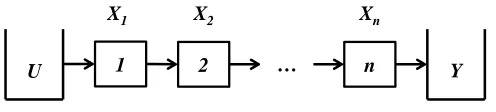
3.3.1.Modeling ‘n’ serial stations
15 Yk, and Xi,k be the time at which the incoming parts are made available to the line, the time at which the finished product leaves the line and the starting time of processing on the ithstation for the kth job respectively.
Figure 3.1 Flow line with n serial stations
For station 1 to start processing the kth job, the following conditions must be fulfilled: 1) Arrival of incoming parts for the kth job, and 2) Completion of processing the k-1th job. If t1is the processing time for station 1, then these conditions are translated into the following equation:
𝑋1,𝑘= 𝑚𝑎𝑥( 𝑡1+ 𝑋1,𝑘−1, 𝑈𝑘) (3.1)
which is presented in the max-plus algebra as:
𝑋1,𝑘= 𝑡1𝑋1,𝑘−1⊕ 𝑈𝑘 (3.2)
Similarly, for any station i the conditions are: 1) End of processing the kth job on the i-1th station, and 2) End of processing the k-1th job on ith station. These are expressed in max-plus algebra as:
𝑋𝑖,𝑘 = 𝑡𝑖𝑋𝑖,𝑘−1⊕ 𝑡𝑖−1𝑋𝑖−1,𝑘 (3.3)
Combining equations (3.2) and (3.3) in matrix form yields:
𝑿𝑘 = 𝑨 𝑿𝑘⊕ 𝑩 𝑿𝑘−1 ⊕ 𝑫 𝑼𝑘 (3.4)
where,
𝑿𝑘 = [
𝑋1,𝑘
𝑋2,𝑘
⋮
𝑋𝑛,𝑘
] , 𝑨 = [
𝜀 𝜀 … 𝜀
𝑡1 𝜀 … 𝜀
⋱ ⋮
𝜀 𝜀 𝑡𝑛−1 𝜀
], 𝑩 = [
𝑡1 𝜀 𝜀
𝜀 𝑡2 𝜀
⋮ ⋱ ⋮
𝜀 𝜀 … 𝑡𝑛
], and 𝑫 = [
𝑒 𝜀 ⋮ 𝜀
].
Following theorem (2.1), equation (3.4) can be written as:
𝑿𝑘 = 𝑨̂ 𝑿𝑘−1 ⊕ 𝑩̂ 𝑼𝑘 (3.5)
1 2 … n
U Y
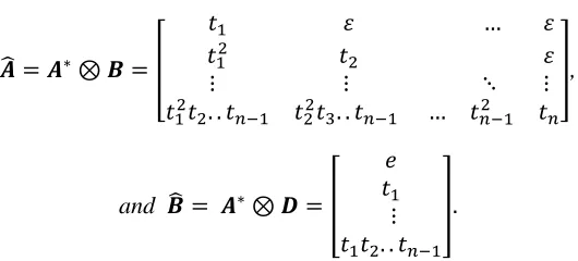
16 where:
𝑨̂ = 𝑨∗⊗ 𝑩 = [
𝑡1 𝜀 … 𝜀
𝑡12 𝑡
2 𝜀
⋮ ⋮ ⋱ ⋮
𝑡12𝑡
2. . 𝑡𝑛−1 𝑡22𝑡3. . 𝑡𝑛−1 … 𝑡𝑛−12 𝑡𝑛
],
and 𝑩̂ = 𝑨∗⊗ 𝑫 = [
𝑒
𝑡1
⋮
𝑡1𝑡2. . 𝑡𝑛−1
].
From equation (3.5) it can be deduced that for any station i, the starting time for the kth job is equal to:
𝑋𝑖,𝑘 = 𝑡𝑖𝑋𝑖,𝑘−1 ⊕ 𝑡𝑖−12 𝑋𝑖−1,𝑘−1⊕ 𝑡𝑖−22 𝑡𝑖−1𝑋𝑖−2,𝑘−1
⊕ … ⊕ 𝑡12𝑡
2… 𝑡𝑖−1𝑋1,𝑘−1⊕ 𝑡1𝑡2… 𝑡𝑖−1𝑈𝑘 (3.6)
Since equations (3.5) and (3.6) were generated for a general serial flow line, they can be used to directly generate the max-plus equations for serial lines with any number of stages given the number of stations in the line.
3.3.2.Modeling ‘n’ merging lines
Merging lines are common in assembly flow lines. A merging station requires input from more than one station or line and delivers one output to the next station. Figure 3.2 shows n stations, each with its own input of incoming parts, merging into one station.
Figure 3.2 Flow line with n merging lines
If tiis the processing time for station i, and Ui,k is the time at which incoming parts are made available for the 1i
th
station, then equation (3.2) holds for any station 1iand the conditions for
U1
U2
…
Un
11
12
1n
2 Y
X1n
X12
X11
17 station 2 to start processing are: 1) End of processing the kth job on stations 1i (i = 1→n ), and 2) End of processing the k-1th job on station 2. Accordingly, the max-plus equations for the system in figure 3.2 can be presented as:
𝑿𝑘 = 𝑨 𝑿𝑘⊕ 𝑩 𝑿𝑘−1 ⊕ 𝑫 𝑼𝑘 (3.7)
where, 𝑿𝑘 = [ 𝑋11,𝑘 𝑋12,𝑘 ⋮ 𝑋1𝑛,𝑘
𝑋2,𝑘]
, 𝑼𝑘 = [ 𝑈1,𝑘 𝑈2,𝑘 ⋮ 𝑈𝑛,𝑘] , 𝑨 = [ 𝜀 𝜀 … 𝜀 ⋮ ⋮ … ⋮ ⋱ 𝜀 𝜀 𝜀 𝜀
𝑡1 𝑡2 … 𝑡1𝑛 𝜀]
, 𝑩 =
[
𝑡11 𝜀 … 𝜀
𝜀 𝑡12 𝜀 … 𝜀
⋮ 𝜀 ⋱ ⋮
⋮ 𝑡1𝑛 𝜀
𝜀 𝜀 … 𝜀 𝑡2]
, and 𝑫 =
[ 𝑒 𝜀 … 𝜀 𝜀 𝑒 𝜀 … 𝜀 ⋮ 𝜀 ⋱ ⋮ 𝜀 ⋮ 𝑒 𝜀 𝜀 𝜀 … 𝜀 𝜀 ] .
Again following theorem (2.1), equation (3.7) becomes:
𝑿𝑘 = 𝑨̂ 𝑿𝑘−1 ⊕ 𝑩̂ 𝑼𝑘 (3.8)
where:
𝑨̂ =
[
𝑡11 𝜀 … 𝜀
𝜀 𝑡12 𝜀
⋮ ⋱ ⋮
𝜀 𝜀 𝑡1𝑛 𝜀
𝑡112 𝑡
122 … 𝑡1𝑛2 𝑡2]
, and 𝑩̂ =
[
𝑒 𝜀 … 𝜀
𝜀 𝑒 ⋮
⋮ ⋱
𝜀 𝜀 𝑒 𝜀
𝑡11 𝑡12 … 𝑡1𝑛]
.
From equation (3.8) it can be deduced that for any station 1i, the starting time for the kth job is equal to:
𝑋1𝑖,𝑘 = 𝑡1𝑖𝑋𝑖,𝑘−1⊕ 𝑈𝑖 (3.9)
and for station 2, the starting time for the kthtime is equal to:
𝑋2,𝑘= 𝑡112 𝑋11,𝑘−1⊕ 𝑡122 𝑋12,𝑘−1⊕ … ⊕ 𝑡2𝑋2,𝑘−1⊕ 𝑡11𝑈1,𝑘⊕ 𝑡12𝑈2,𝑘⊕ …
18 Equations (3.8), (3.9), and (3.10) can similarly be used to directly generate the max-plus equations for any number of merging lines.
From equations (3.9) and (3.10) it can be observed that the equation for merging lines is just a concatenation of the equations of several serial lines. Therefore, using equations (3.6) and (3.10) the 𝑨 ̂and 𝑩̂ matrices can be constructed for any structure of flow lines with infinite buffers and no parallel identical stations at any stage.
3.3.3.Modeling parallel identical stations
Adding parallel identical stations is a common method for increasing capacity and throughput in flow lines. Modeling parallel identical stations in max-plus algebra is not straight forward as it represents a logical OR in the system where jobs arriving at the stage with parallel identical stations can go to one of the stations OR another. In max-plus algebra, modeling logical OR requires modeling all possible cases which increases the size of the model exponentially with the number of jobs. One possible approximation to make, in order to model n parallel identical stations, is to transform them into n serial ones each with a processing time of t/n, where t is the processing time of the parallel identical stations. This approximation will result in equal average throughput but not accurate starting and finishing times for stations.
Figure 3.3 shows a three stage flow line with n parallel identical stations in the second stage. For the stations in the first and third stages to start working on the kth job, the same conditions mentioned in section 3.3.1 are required. However, for a station in the second stage, the condition that the station should have finished processing the k-1th job is not required as there are parallel stations that can process the job. Alternatively, all the parallel identical stations in the second stage can be regarded as one station with processing time 𝑡2 and capacity of n jobs. Thus the condition that the station should have finished processing the k-1th job would be replaced by a condition that processing the k-nth job has ended. Thus, the model equations for the system in figure 3.3 would be:
𝑿𝑘 = 𝑨 𝑿𝑘⊕ 𝑩𝟏 𝑿𝑘−1 ⊕ 𝑩𝟐 𝑿𝑘−𝑛 ⊕ 𝑫 𝑼𝒌 (3.11)
where:
𝑩𝟏 = [
𝑡1 𝜀 𝜀
𝜀 𝜀 𝜀
𝜀 𝜀 𝑡3] and 𝑩𝟐 = [
𝜀 𝜀 𝜀
𝜀 𝑡2 𝜀
19 Using theorem (2.1), equation (3.11) can then be written as:
𝑿𝑘= 𝑨̂ 𝑿𝑘−1 ⊕ 𝑨𝑷̂𝟐 𝑿𝑘−𝑛⊕ 𝑩̂ 𝑈𝑘 (3.12)
where:
𝑨̂ = 𝑨∗⊗ 𝑩
𝟏= [
𝑡1 𝜀 𝜀
𝑡12 𝜀 𝜀
𝑡12𝑡
2 𝜀 𝑡3
] , 𝑩̂ = 𝑨∗⊗ 𝑫 = [
𝑒
𝑡1
⋮
𝑡1𝑡2. . 𝑡𝑛−1
],
and 𝑨𝑷̂𝟐= 𝑨∗⊗ 𝑩𝒏= [
𝜀 𝜀 𝜀
𝜀 𝑡2 𝜀
𝜀 𝑡22 𝜀].
Figure 3.3 A three stage flow line with n parallel identical stations in the second stage.
By examining equations (3.5) and (3.12), the following can be observed: first, matrix 𝑩̂ is unchanged; second, matrix 𝑨̂is unchanged except for taking out the column corresponding to the stage where parallel stations are added and replacing it by a column of ‘𝜀’s; third, the column removed from matrix 𝑨̂ is placed in a the same position in another matrix of ‘𝜀’s and multiplied by 𝑿𝑘−𝑛.
Thus in order to model parallel identical stations in one stage, it is assumed that only one station exists and the equations are generated as per section 3.3.1 or 3.3.2 then the column corresponding to the stage with parallel stations in matrix 𝑨̂ is replaced by a column of ‘𝜀’s, then is inserted in another matrix 𝑨𝑷̂ and multiplied by the vector 𝑿𝑘−𝑛 where n is the number of parallel identical stations in that stage.
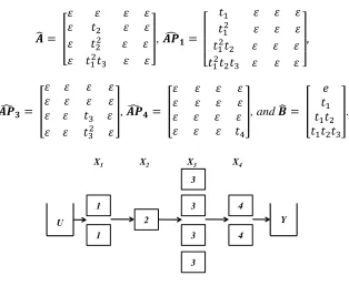
To demonstrate, assume a system as in figure 3.4 where all the parallel stations are identical and jobs arriving at each stage can be served by any station. The system is first assumed to be a serial
U Y
X1 X3
1
X2
22
2n
21
3
20 line with four stages and one station in each stage. Accordingly, following equation (3.5), the 𝑨̂ matrix will be:
𝑨̂ =
[
𝑡1 𝜀 𝜀 𝜀
𝑡12 𝑡
2 𝜀 𝜀
𝑡12𝑡
2 𝑡22 𝑡3 𝜀
𝑡12𝑡
2𝑡3 𝑡12𝑡3 𝑡32 𝑡4] .
Using the generated matrix 𝑨̂, the equations describing that system can be directly generated as:
𝑿𝑘 = 𝑨̂ 𝑿𝑘−1 ⊕ 𝑨𝑷̂𝟏 𝑿𝑘−2⊕ 𝑨𝑷̂𝟑 𝑿𝑘−4⊕ 𝑨𝑷̂𝟒 𝑿𝑘−2⊕ 𝑩̂ 𝑈𝑘 (3.13)
where:
𝑨̂ = [
𝜀 𝜀 𝜀 𝜀
𝜀 𝑡2 𝜀 𝜀
𝜀 𝑡22 𝜀 𝜀
𝜀 𝑡12𝑡
3 𝜀 𝜀
], 𝑨𝑷̂𝟏 =
[
𝑡1 𝜀 𝜀 𝜀
𝑡12 𝜀 𝜀 𝜀
𝑡12𝑡
2 𝜀 𝜀 𝜀
𝑡12𝑡2𝑡3 𝜀 𝜀 𝜀 ]
,
𝑨𝑷̂𝟑 = [
𝜀 𝜀 𝜀 𝜀
𝜀 𝜀 𝜀 𝜀
𝜀 𝜀 𝑡3 𝜀
𝜀 𝜀 𝑡32 𝜀
], 𝑨𝑷̂𝟒 = [
𝜀 𝜀 𝜀 𝜀
𝜀 𝜀 𝜀 𝜀
𝜀 𝜀 𝜀 𝜀
𝜀 𝜀 𝜀 𝑡4
], and 𝑩̂ = [
𝑒
𝑡1
𝑡1𝑡2
𝑡1𝑡2𝑡3
].
Figure 3.4 Flow line with parallel identical stations in several stages
It should be noted that equation (3.13) can be simplified by combining the matrices that are multiplied by the same delayed state vector, hence, equation (3.13) becomes:
𝑿𝑘 = 𝑨̂ 𝑿𝑘−1 ⊕ 𝑨𝑷̂𝟏,𝟒 𝑿𝑘−2⊕ 𝑨𝑷̂𝟑 𝑿𝑘−4⊕ 𝑩̂ 𝑈𝑘 (3.14)
where:
1
U Y
X1 X2 X4
21
𝑨̂ = [
𝜀 𝜀 𝜀 𝜀
𝜀 𝑡2 𝜀 𝜀
𝜀 𝑡22 𝜀 𝜀
𝜀 𝑡12𝑡3 𝜀 𝜀
], 𝑨𝑷̂𝟏,𝟒=
[
𝑡1 𝜀 𝜀 𝜀
𝑡12 𝜀 𝜀 𝜀
𝑡12𝑡
2 𝜀 𝜀 𝜀
𝑡12𝑡
2𝑡3 𝜀 𝜀 𝑡4 ]
, 𝑨𝑷̂𝟑=
[
𝜀 𝜀 𝜀 𝜀
𝜀 𝜀 𝜀 𝜀
𝜀 𝜀 𝑡3 𝜀
𝜀 𝜀 𝑡32 𝜀
] , and 𝑩̂ = [
𝑒
𝑡1
𝑡1𝑡2
𝑡1𝑡2𝑡3
].
However, it is better to keep the system equations in the form presented in equation (3.13) as it becomes clearer and easier to adjust the equations if the number of stations in any of these stages is changed.
3.3.4.Modeling finite buffers
To model finite buffers; assume a general station i followed by a buffer with a finite size B. For the kthjob to start on station i an additional condition is required to account for the buffer, which is for station i+1 to have started processing the job number k-B-1. Assuming that station i mentioned above is part of a general flow line, then the line equations will be the same as equation (3.5) with the addition of one term as follows:
𝑿𝑘 = 𝑨̂ 𝑿𝑘−1 ⊕ 𝑩̂ 𝑈𝑘⊕ 𝑨̂𝒊 𝑿𝑘−𝐵−1 (3.15)
where:
𝑨̂𝒊 = 𝑨∗⊗ 𝑨
𝒊, and 𝑨𝒊 =
[
𝜀 … 𝜀 𝜀 … 𝜀
⋮ ⋮ ⋮ ⋮
𝜀
𝜀 … 𝜀 𝑒 𝜀
⋮ ⋮ 𝜀 ⋮ ⋮
⋮
𝜀 … 𝜀 𝜀 𝜀 𝜀]
,
where 𝑨𝒊is a null matrix with only one e located at the ith row and the i+1th column.
22
𝑿𝑘 = 𝑨̂ 𝑿𝑘−1 ⊕ 𝑩̂ 𝑼𝑘⊕ 𝑨𝑩̂𝟐 𝑿𝑘−𝐵2−1⊕ 𝑨𝑩̂𝟑 𝑿𝑘−𝐵3−1
⊕ 𝑨𝑩̂𝟒 𝑿𝑘−𝐵4−1 (3.16)
where 𝑨̂and 𝑩̂ are the same as in equation (3.5),
𝑨𝑩̂𝟐= [
𝜀 𝑒 𝜀 𝜀
𝜀 𝑡1 𝜀 𝜀
𝜀 𝑡1𝑡2 𝜀 𝜀
𝜀 𝑡1𝑡2𝑡3 𝜀 𝜀
], 𝑨𝑩̂𝟑 = [
𝜀 𝜀 𝜀 𝜀
𝜀 𝜀 𝑒 𝜀
𝜀 𝜀 𝑡2 𝜀
𝜀 𝜀 𝑡2𝑡3 𝜀
],and
𝑨𝑩̂𝟒= [
𝜀 𝜀 𝜀 𝜀
𝜀 𝜀 𝜀 𝜀
𝜀 𝜀 𝜀 𝑒
𝜀 𝜀 𝜀 𝑡3
].
Figure 3.5 Flow line with 4 serial stations and 3 finite buffers.
By examining equation (3.16), it is clear that the model of a finite buffer between two stations i and j uses the same equations for lines without the buffer with the addition of another matrix multiplied by vector 𝑿𝑘−𝐵−1 where B is the buffer size and this matrix is a Null matrix except for the jth column which is equal to the column corresponding to station i in the 𝑨̂matrix divided by the processing time of station i.
3.3.5.Modeling general flow lines
An algorithm is presented for the automatic generation of the max-plus equations for a general flow line as follows:
Step 1: Simplify the flow line to be modelled by assuming infinite buffers and no parallel identical stations.
Step 2: Encode the simplified flow line into an adjacency matrix while assuming the line to be an undirected graph.
1
U Y
X1 X2 X4
2 3 4
X3
23 Step 3: Re-arrange the rows and columns of the matrix and identify merging stations according to the rank order clustering technique.
Step 4: Arrange 𝑋𝑖 in the vector 𝑿 according to the new order of stations in the adjacency matrix, where i is the total number of stations in the line excluding parallel identical ones.
Step 5: Generate the 𝑨̂ and 𝑩̂ matrices for the simplified flow line according to equations (3.6) and (3.10).
Step 6: Take into account parallel identical stations by altering the 𝑨̂ matrix and adding new matrices for each stage with parallel identical stations as described in section 3.3.3.
Step 7: Finalize the equations by accounting for finite buffers as described in section 3.3.4.
To demonstrate how the algorithm works consider the flow line shown in figure 3.6 (a) which includes parallel identical stations in stages C and B and finite buffers 𝑏1, 𝑏2 and 𝑏3with sizes 2, 2 and 4 respectively.
In step 1 the flow line in figure 3.6 (a) is transformed into that in figure 3.6 (b) with all buffers removed and parallel identical stations replaced by only one station.
24
Figure 3.6 General flow line. (a) Line with parallel identical machines and buffers. (b) Line after simplification.
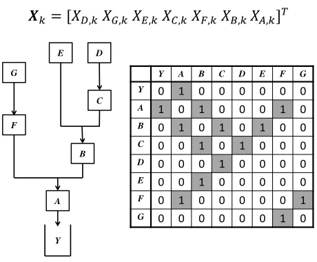
From the adjacency matrix in figure 3.8 and following step 4, the starting times vector of the different stations is given by:
𝑿𝑘 = [𝑋𝐷,𝑘 𝑋𝐺,𝑘 𝑋𝐸,𝑘 𝑋𝐶,𝑘 𝑋𝐹,𝑘 𝑋𝐵,𝑘 𝑋𝐴,𝑘]𝑇
Figure 3.7 A general flow line and its corresponding adjacency matrix.
A
Y
E D
F G
C2 C1
b2 b1
b3 B2 B3 B1
A
Y B
C
E D
F G
(a) (b)
U3
U2 U1
U3
U2 U1
A
Y B
C
E D
F
G Y A B C D E F G
25
Figure 3.8 Adjacency matrix and its corresponding flow line diagram after re-arranging the rows and columns of the
matrix
Following step 5, the ordered adjacency matrix is used along with equations (3.6), (3.9) and (3.10) to generate the 𝑨̂ and 𝑩̂ matrices for the simplified flow line. This step is automated and performed using the symbolic mathematical solver Wolfram Mathematica 6.0 (Grzymkowski, Kapusta et al. 2008) and the generated matrices are:
𝑨̂ =
[
𝑡𝐷 𝜀 … 𝜀
𝜀 𝑡𝐺 𝜀
𝜀 𝜀 𝑡𝐸 𝜀
𝑡𝐷2 𝜀 𝜀 𝑡
𝐶 𝜀 ⋮
𝜀 𝑡𝐺2 𝜀 𝜀 𝑡
𝐹 𝜀
𝑡𝐷2𝑡
𝐶 𝜀 𝑡𝐸2 𝑡𝐶2 𝜀 𝑡𝐵 𝜀
𝑡𝐷2𝑡
𝐶𝑡𝐵 𝑡𝐺2𝑡𝐹 𝑡𝐸2𝑡𝐵 𝑡𝐶2𝑡𝐵 𝑡𝐹2 𝑡𝐵2 𝑡𝐴]
, and 𝑩̂ =
[
𝑒 𝜀 𝜀
𝜀 𝜀 𝑒
𝜀 𝑒 𝜀
𝑡𝐷 𝜀 𝜀
𝜀 𝜀 𝑡𝐺
𝑡𝐷𝑡𝐶 𝑡𝐸 𝜀
𝑡𝐷𝑡𝐶𝑡𝐵 𝑡𝐸𝑡𝐵 𝑡𝐺𝑡𝐹]
.
Next, the parallel identical stations at stations B and C are modelled. Following section 3.3.3, the equation for the line while taking into account the parallel identical stations becomes:
𝑿𝑘 = 𝑨𝟏̂ 𝑿𝑘−1 ⊕ 𝑨𝑷̂𝑪 𝑿𝑘−2⊕ 𝑨𝑷̂𝑩 𝑿𝑘−3⊕ 𝑩̂ 𝑈𝑘 (3.17)
where:
Y A B F C E G D
Y 0 1 0 0 0 0 0 0
A 1 0 1 1 0 0 0 0
B 0 1 0 0 1 1 0 0
F 0 1 0 0 0 0 1 0
C 0 0 1 0 0 0 0 1
E 0 0 1 0 0 0 0 0
G 0 0 0 1 0 0 0 0
D 0 0 0 0 1 0 0 0
A
Y B
C E
D
26 𝑨𝟏̂ = [ 𝑡𝐷 𝜀 … 𝜀 𝜀 𝑡𝐺 𝜀 𝜀 𝜀 𝑡𝐸 𝜀
𝑡𝐷2 𝜀 𝜀 𝜀 𝜀 ⋮
𝜀 𝑡𝐺2 𝜀 𝜀 𝑡
𝐹 𝜀
𝑡𝐷2𝑡𝐶 𝜀 𝑡𝐸2 𝜀 𝜀 𝜀 𝜀
𝑡𝐷2𝑡
𝐶𝑡𝐵 𝑡𝐺2𝑡𝐹 𝑡𝐸2𝑡𝐵 𝜀 𝑡𝐹2 𝜀 𝑡𝐴]
, 𝑨𝑷̂𝑪= [ 𝜀 𝜀 … 𝜀 𝜀 𝜀 𝜀 𝜀 𝜀 𝜀 𝜀 𝜀 𝜀 𝜀 𝑡𝐶 𝜀 ⋮ 𝜀 𝜀 𝜀 𝜀 𝜀 𝜀
𝜀 𝜀 𝜀 𝑡𝐶2 𝜀 𝜀 𝜀
𝜀 𝜀 𝜀 𝑡𝐶2𝑡
𝐵 𝜀 𝜀 𝜀] , 𝑨𝑷̂𝑩= [ 𝜀 𝜀 … 𝜀 𝜀 𝜀 𝜀 𝜀 𝜀 𝜀 𝜀 𝜀 𝜀 𝜀 𝜀 𝜀 ⋮ 𝜀 𝜀 𝜀 𝜀 𝜀 𝜀 𝜀 𝜀 𝜀 𝜀 𝜀 𝑡𝐵 𝜀
𝜀 𝜀 𝜀 𝜀 𝜀 𝑡𝐵2 𝜀]
, and 𝑩̂ =
[ 𝑒 𝜀 𝜀 𝜀 𝜀 𝑒 𝜀 𝑒 𝜀 𝑡𝐷 𝜀 𝜀 𝜀 𝜀 𝑡𝐺 𝑡𝐷𝑡𝐶 𝑡𝐸 𝜀 𝑡𝐷𝑡𝐶𝑡𝐵 𝑡𝐸𝑡𝐵 𝑡𝐺𝑡𝐹] .
The final step is then to include the finite buffers by augmenting equation (3.17) with the matrices
𝑨𝑩̂𝑭, 𝑨𝑩̂𝑩and 𝑨𝑩̂𝑨multiplied by 𝑿𝑘−2−1, 𝑿𝑘−2−1 and 𝑿𝑘−4−1 respectively according to section 3.3.4. The final equations then become:
𝑿𝑘 = 𝑨𝟏̂ 𝑿𝑘−1 ⊕ 𝑨𝑷̂𝑪 𝑿𝑘−2⊕ 𝑨𝑷̂𝑩 𝑿𝑘−3⊕ 𝑨𝑩̂𝑭 𝑿𝑘−3⊕ 𝑨𝑩̂𝑩 𝑿𝑘−3
⊕ 𝑨𝑩̂𝑨 𝑿𝑘−5⊕ 𝑩̂ 𝑈𝑘 (3.18)
where 𝑨𝟏̂, 𝑨𝑷̂𝑪, 𝑨𝑷̂𝑩, and 𝑩̂are the same as in equation (3.17) and:
27
[
𝜀 𝜀 𝜀 𝜀 𝜀 𝜀 𝜀
𝜀 𝜀 𝜀 𝜀 𝜀 𝜀 𝜀
𝜀 𝜀 𝜀 𝜀 𝜀 𝑒 𝜀
𝜀 𝜀 𝜀 𝜀 𝜀 𝑒 𝜀
𝜀 𝜀 𝜀 𝜀 𝜀 𝜀 𝜀
𝜀 𝜀 𝜀 𝜀 𝜀 𝑡𝐸⊕ 𝑡𝐶 𝜀
𝜀 𝜀 𝜀 𝜀 𝜀 (𝑡𝐸⊕ 𝑡𝐶)𝑡𝐵 𝜀 ]
,and
𝑨𝑩̂𝑨=
[
𝜀 𝜀 𝜀 𝜀 𝜀 𝜀 𝜀
𝜀 𝜀 𝜀 𝜀 𝜀 𝜀 𝜀
𝜀 𝜀 𝜀 𝜀 𝜀 𝜀 𝜀
𝜀 𝜀 𝜀 𝜀 𝜀 𝜀 𝜀
𝜀 𝜀 𝜀 𝜀 𝜀 𝜀 𝑒
𝜀 𝜀 𝜀 𝜀 𝜀 𝜀 𝑒
𝜀 𝜀 𝜀 𝜀 𝜀 𝜀 𝑡𝐵⊕ 𝑡𝐹]
.
It should be noted that changing the number of parallel identical stations or buffer size for the finite buffers in equation (3.18) requires only changing the number subtracted from state vector multiplied by the corresponding matrix. For example changing the size of buffer 𝑏3from 4 to 6 will only change the term 𝑨𝑩̂𝑨 𝑿𝑘−5 in equation (3.18) to 𝑨𝑩̂𝑨 𝑿𝑘−7.
3.4.
Case Study and Analysis
A case study is presented where three possible assembly system configurations for a back flushing control valve are modeled, analyzed and compared using max-plus equations generated by the developed method. Assembly lines for valves can be automated lines with moving pallets similar to the system presented in figure 3.9.
28 Figure 3.10 presents the 8 components of the back flushing control valve (Dorot (2001)). The assembly sequence tree of the valve (Kashkoush and ElMaraghy 2014) is presented in figure 3.11 (a) along with three possible assembly line configurations as shown in figure 3.11 (b, c and d). In the assembly sequence tree, each node represents an independent subassembly, therefor; assembling components 1 and 2 and components 6 and 7 and components 3 and 4 can all start simultaneously as no precedence relationship exists between them. Translating assembly sequences into possible line configurations depends on many factors such as available space, available number of workers, required tools for each operation etc. This is done using techniques for planning plant layout including optimization analysis.
The main component of the valve is the body which is component 3. Components 1 and 2, the bonnet and diaphragm are assembled to one side of the body while the rest of the components are assembled from the opposite side. The assembly line starts with the valve body moving on a pallet, the first assembly operation is to add component 4 which is the seat to the body then component 5; the guide cone, is added to the previous subassembly. In the next operation, the subassembly of components 6 and 7, which is already sub-assembled in a different station, is added to the body subassembly. Then component 8, the adapter, is added to the body subassembly and the valve is inverted to assemble the rest of the components on the opposite side. The final assembly operation is then to add the subassembly of components 1 and 2 to the body. All assembly operations are manual except for inverting the valve which is done by a robot.
The assembly line configurations in figure 3.11 (b) follow the same assembly sequence mentioned above but differ in assigning different operations to different stations. The assembly operations at each station and the corresponding required time for each configuration are given in table 3.1.
29
Figure 3.10 Back flushing control valve components (Dorot (2001)).
Figure 3.11 Assembly sequence tree (Kashkoush and ElMaraghy 2014) (a) and three possible corresponding assembly
line configurations (b).
Following the procedure in section 3.3, the max-plus equations for three configurations, assuming buffers with equal sizes between all stations, are:
𝑿𝑘 = 𝑨̂ 𝑿𝑘−1 ⊕ 𝑨𝑩̂ 𝑿𝑘−𝑏 ⊕ 𝑩̂ 𝑼𝑘 (3.19)
where for configuration 1 𝑿 = [𝑋𝐶 𝑋𝐷 𝑋𝐵 𝑋𝐸 𝑋𝐴 𝑋𝐹]𝑇, for configuration 2
𝑿 = [𝑋𝐶∗ 𝑋𝐵 𝑋𝐸∗ 𝑋𝐴 𝑋𝐹]𝑇 and for configuration 3 𝑿 = [𝑋𝐶 𝑋𝐷 𝑋𝐵 𝑋𝐸 𝑋𝐺 𝑋𝐴 𝑋𝐹]𝑇. The values of
𝑨̂, 𝑨𝑩̂ and 𝑩̂for each of the configurations are given in appendix C.
Back Flushing Control Valve - 57
Body Diaphragm Bonnet
Adapter Seal Bowl
Seal Seat
Guide Cone 1
2
3
4
5
8 7
30
Table 3-1 Assembly processes and required processing times for stations in Figure 3.11 (b).
Station
Assembly processes
Required time in seconds
A Assemble Bonnet and Diaphragm (Parts1 & 2) tA = 43
B Assemble Seal and Seal Bowl (Parts 6 &7)
tB = 15
C Assemble Body and Seat (Parts 3 &4)
tC = 20
D Add Guide cone to Body and Seat (Part 5)
tD = 6
E Assemble Body subassembly with Seal subassembly then add the Adapter
(Assemble (3,4,5) & (6,7) then add 8)
tE = 25
F Add Bonnet and Diaphragm to the assembly (Add (1,2) to (3,4,5,6,7,8) )
tF = 21
C* Assembly Body and Seat then add Guide cone. (Assemble 3 & 4 then add 5)
tC* = 28
E* Assemble Body subassembly with Seal subassembly
(Assemble (3,4,5) & (6,7))
tE* = 18
G Add Adapter to Body and Seal subassembly (Add 8 to (3,4,5,6,7))
tG = 5
Using equation (3.19) and assuming 𝑼𝑘 is given, the exact starting times for every station for every job can be obtained, where the kth starting time on station m is given by 𝑋𝑚,𝑘. For example, assuming stations A, B and C are never starved ( i.e. 𝐔𝟏= [𝟎 𝟎 𝟎]𝐓 and Uk≤ [XC XB XA]k−1T +
[tC tB tA]T) and starting from an empty line (