ABSTRACT
WANG, SHU. Reliability Assessment of Power Systems with Wind Power Generation. (Under the direction of Dr. Mesut E Baran.)
Wind power generation, the most promising renewable energy, is increasingly attractive to power industry and the whole society and becomes more significant in the portfolio of generation systems. However, because of the unfavorable features of wind power, it affects all aspects of traditional processes of power system planning and operation. Power systems primarily planned for providing reliable and economic electric power to their customers. Therefore, it is critical to assess and understand the impacts of wind power on power system reliability.
Reliability Assessment of Power Systems with Wind Power Generation
by Shu Wang
A thesis submitted to the Graduate Faculty of North Carolina State University
In partial fulfillment of the Requirements for the degree of
Master of Science
Electrical Engineering
Raleigh, North Carolina 2008
APPROVED BY:
_______________________________ ______________________________
Dr. Mesut E Baran Dr. Alex Q. Huang
Committee Chair
DEDICATION
To Dong
For my wonderful wife
For our everlasting love
BIOGRAPHY
Shu Wang was born in Tianjin, China in 1978. He earned his Bachelor degree and Master degree both in Electrical Engineering and Automation from Tianjin University in Tianjin, China, in 2001 and 2004, respectively. In July 2004, he left his home town the place he spent 25 years since childhood and came to the United State to embark on his splendid venture overseas.
From August 2004 to June 2005, he studied as a graduate student in the Department of Electrical and Computer Engineering of the University of Texas at Austin where he started the interests in wind power and long-horn football game. He worked as an intern in Entergy Corporation in the summer of 2005 in New Orleans, Louisiana. He mainly worked on the Eastern Interconnection Phasor Project (EIPP), a project about Phasor Measurement Unit (PMU) and its applications. From August 2005, he became a full time consulting engineer in Electric System Consulting of ABB Inc. He is the main designer and developer of GridView, the popular power market simulation software in US. He also involves in various kinds of studies related to energy market. In summer 2006, he continued his graduate study in the Department of Electrical and Computer Engineering of North Carolina State University. During the thesis study, under the direction of Dr. Mesut Baran, he researched the impact of wind generation on reliability of bulk power systems and developed a Monte Carlo based production cost simulation model.
ACKNOWLEDGMENTS
I am sincerely grateful to my advisor, Dr. Mesut Baran for his critical guidance, patience, and inspiration throughout my thesis process. Thank you for imparting your comprehensive knowledge and sharing your wisdom. Completing this thesis with you has certainly been an honor for me.
I would also like to thank my committee members, Dr. Alex Huang and Dr. Subhashish Bhattacharya for the considerations and suggestions on my thesis.
I would also like to thank the technical and financial supports from Electric System Consulting of ABB Inc. during my graduate studies. Particularly, based on his rich experience in power industry, Dr. Jinxiang Zhu gave me plenty of valuable advice for my thesis.
Last but not least, I must appreciate my mother who always believes in me and enlightens me to be a good man. The intelligence and fortitude inherited from her make every success of mine.
TABLE OF CONTENTS
LIST OF TABLES ... vii
LIST OF FIGURES ... viii
Chapter 1 Introduction ... 1
1.1. Development of Wind Power in United States ... 1
1.2. Wind Power Generation Pros and Cons ... 3
1.3. Impact of Wind Power on Power System Planning and Operation ... 5
1.4. Wind Generation Integration Issues ... 9
1.5. Thesis Overview ... 10
1.6. Abbreviations ... 11
Chapter 2 Power System Reliability ... 13
2.1. Concept of Power System Reliability ... 13
2.2. Reliability Evaluation Methodology ... 14
2.2.1. Analytical Method ... 14
2.2.2. Monte Carlo Simulation Based Method ... 17
2.2.2.1. Power System Operations ... 18
2.2.2.2. Unit Commitment ... 21
2.2.2.3. Reliability Assessment ... 23
Chapter 3 Wind Power Generation Fundamentals ... 25
3.1. Wind Power Production ... 25
3.2. Impacts on Power Systems ... 27
3.2.1. Under forecast of wind generation ... 28
3.2.2. Over Forecast of Wind Generation ... 28
3.3. Wind Energy Forecasting ... 29
3.3.1. Importance of Wind Forecasting ... 30
3.3.2. Wind Forecasting Methodology ... 31
3.3.3. Time Series Models ... 33
3.4. Capacity Value of Wind Power ... 34
3.4.1. Methodologies for Capacity Value Estimation of A WTGS ... 35
3.4.1.1. Effective Load Carrying Capability (ELCC) ... 36
3.4.1.2. Equivalent Conventional Generating Unit ... 37
3.4.1.3. Customized Capacity Factor Method ... 38
Chapter 4 Reliability Assessment of Power Systems with Wind Power Generation .. 39
4.1. Introduction ... 39
4.2. Monte Carlo Based Production Cost Simulation Model ... 40
4.2.1. Model Input and Output ... 42
4.2.2. Daily Loop for Day-ahead Unit Commitment ... 43
4.2.2.1. Variable Cost of Generating Units ... 45
4.2.2.2. Generator Availability ... 46
4.2.2.3. Commitment Decision ... 48
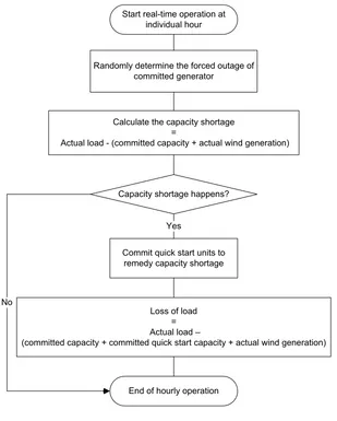
4.2.3. Hourly Loop for Real-time Operation ... 50
4.2.3.1. Generator Forced Outage ... 52
4.2.3.2. Real-time Generating Resource Adequacy ... 53
4.2.3.3. Commitment of Quick Start Units ... 53
4.2.3.4. Loss of Load Calculation ... 56
4.3. Day-ahead Hourly Wind Generation Forecasting ... 56
4.3.1. Automatic Forecasting Process Details ... 58
4.3.2. Individual Day-ahead Forecast Using ARMA ... 60
4.3.2.1. Identification ... 61
4.3.2.2. Estimation... 63
4.3.2.3. Forecasting ... 66
4.3.3. Day-ahead Forecasting through Simulation Period ... 68
4.4. Verification of the Monte Carlo Simulation Model ... 72
4.4.1. Load Model of RTS ... 72
4.4.2. Generating System of RTS ... 73
4.4.3. Reliability Evaluation of RTS ... 74
4.4.4. Reliability Evaluation of RTS with Wind Power Generation ... 76
Chapter 5 Case Study ... 79
5.1. General Description of the Study System ... 79
5.1.1. System Load Profile ... 80
5.1.2. Conventional Generating System ... 81
5.1.3. Wind Power Generation System ... 86
5.2. Base case Reliability ... 90
5.3. Wind Generation Integration ... 92
5.3.1. Economic Analysis ... 95
5.3.2. Generator Utilization ... 97
5.4. Reserve Requirement Adjustment ... 99
5.5. Impact of Quality of Wind Generation Forecasting on Reliability ... 100
5.6. Capacity Value Evaluation ... 102
5.6.1. Effective Load Carrying Capability (ELCC) ... 104
5.6.2. Equivalent Conventional Generating Unit ... 106
5.6.3. Customized Capacity Factor Method ... 107
Chapter 6 Conclusions and Future Work ... 110
6.1. Conclusions ... 110
6.2. Suggestions for Future Work ... 111
REFERENCES ... 113
LIST OF TABLES
Table 2-1 Capacity outage probability table ... 16
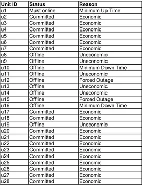
Table 4-1 Commitment status of units ... 49
Table 4-2 Data range of each forecasting process ... 57
Table 4-3 Statistics of the one week hourly historical wind generation ... 61
Table 4-4 Autocorrelation check for white noise ... 63
Table 4-5 ARMA model estimation ... 64
Table 4-6 Autocorrelation check of residuals ... 65
Table 4-7 Forecasting performance comparison of ARMA models ... 69
Table 4-8 Generating system information of RTS ... 74
Table 4-9 Reliability indices comparison ... 74
Table 4-10 Reliability indices of 10% penetration case and 30% penetration case ... 77
Table 5-1 Summary of generation resource in study system ... 82
Table 5-2 Detailed data of generation system ... 83
Table 5-3 Availability statistics of coal-fired generating units in GADS ... 84
Table 5-4 Data for quick start units in the study system... 86
Table 5-5 Installed capacity of wind projects ... 86
Table 5-6 Reliability indices of base case ... 91
Table 5-7 Installed capacity for wind penetration scenarios ... 93
Table 5-8 Reliability indices for different wind penetration cases ... 93
Table 5-9 Production cost analysis for different wind penetration cases ... 96
Table 5-10 Penalty cost of load shedding for different wind penetration cases ... 96
Table 5-11 Generator utilization for different wind penetration cases ... 98
Table 5-12 Reliability indices using different wind forecasting methods ... 101
Table 5-13 Data of equivalent thermal unit ... 106
LIST OF FIGURES
Figure 1-1 Wind power generation in United States ... 2
Figure 1-2 Wind resource atlas in Unite States ... 2
Figure 1-3 Unfavorable daily wind generation pattern ... 5
Figure 1-4 Time frames for power systems planning and operation ... 8
Figure 2-1 Two-state model of a unit availability ... 15
Figure 2-2 Scheduling timeline ... 20
Figure 3-1 Power curve of GE 3.6 MW offshore wind turbine ... 26
Figure 3-2 Wind farm configuration ... 27
Figure 3-3 Fast ramp up and down of wind generation ... 29
Figure 3-4 Structure of commercial wind power forecasting tool ... 32
Figure 3-5 ELCC illustration ... 37
Figure 4-1 Main structure of the simulation model ... 41
Figure 4-2 Model input and output ... 42
Figure 4-3 Flow chart of day-ahead unit commitment ... 44
Figure 4-4 Net heat rate of a steam turbine generator ... 46
Figure 4-5 Logic of real-time operation ... 51
Figure 4-6 Logic of commitment of quick start units ... 55
Figure 4-7 Day-ahead forecasts for two consecutive days ... 58
Figure 4-8 Hourly wind generation of Melancthon wind farm... 59
Figure 4-9 Hourly historical wind generation ... 61
Figure 4-10 Analysis of autocorrelations, partial autocorrelations and inverse autocorrelations ... 62
Figure 4-11 White noise tests and unit root tests ... 63
Figure 4-12 Autocorrelations, partial autocorrelations and inverse autocorrelations of residuals ... 65
Figure 4-13 Histogram of residuals ... 66
Figure 4-14 Simulated original data series and forecasted data using estimated ARMA model ... 67
Figure 4-15 Comparison between actual and forecasted hourly wind generation ... 67
Figure 4-16 Forecasting performance comparison of different historical data period ... 70
Figure 4-17 Actual and forecasted wind generation ... 71
Figure 4-18 Histogram of forecast residuals ... 71
Figure 4-19 Load profile of RTS ... 73
Figure 4-20 Reliability indices variation ... 75
Figure 4-21 Histogram of loss of load ... 76
Figure 4-22 Historical and forecasted wind generation ... 77
Figure 4-23 Histogram of loss of load for 30% penetration case ... 78
ix
Figure 4-24 Reliability indices variation for 30% penetration case ... 78
Figure 5-1 Load profile of the study system ... 80
Figure 5-2 Pie chart of the generation resource in study system ... 82
Figure 5-3 System equivalent production cost curve ... 85
Figure 5-4 Monthly average generation of the wind projects ... 87
Figure 5-5 Hourly wind generation of Melancthon I wind project ... 88
Figure 5-6 Hourly wind generation of Kingsbridge I wind project ... 88
Figure 5-7 Hourly wind generation of Erie Shores wind project... 89
Figure 5-8 Hourly wind generation of Prince I & II wind project ... 89
Figure 5-9 Histogram of hourly ramping rate of the aggregated wind generation ... 90
Figure 5-10 Reliability indices variation for base case ... 91
Figure 5-11 Histogram of loss of load for base case ... 91
Figure 5-12 Histogram of loss of load for Quadruple (M+K+E+P) case ... 94
Figure 5-13 Economic benefit analysis for different wind penetration cases ... 97
Figure 5-14 Utilization of quick start units for different wind penetration cases ... 99
Figure 5-15 Reserve requirement adjustment ... 100
Figure 5-16 Historical hourly wind generation of Erie Shores wind project ... 103
Figure 5-17 Monthly average value of wind generation and system load ... 103
Figure 5-18 ELCC analysis for Erie Shore wind project using ARMA forecasting ... 105
Figure 5-19 ELCC analysis for Erie Shore wind project using perfect forecasting ... 106
Figure 5-20 Analysis of equivalent thermal unit method ... 107
Chapter 1
Introduction
1.1. Development of Wind Power in United States
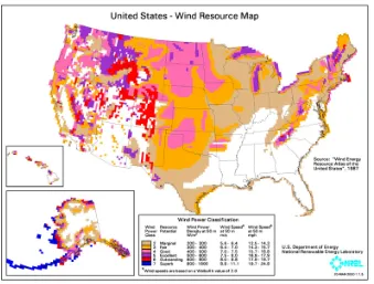
Wind power, the most promising renewable energy, is one of the fastest growing electric generation technologies in United States as well as the whole world. Based on American Wind Energy Association (AWEA) 2008 first quarter market report [1], total installed capacity of wind power throughout United States is 18302 MW and there are 5736 MW wind power projects under construction. Distribution of existing wind power in United States is illustrated in Figure 1-1. Throughout the entire territory of United States, wind energy resource is fairly abundant but not evenly distributed in terms of wind resource atlas in Figure 1-2. The major wind resource concentrated regions include western region, middle region, northwest region, the Great Lakes, the Pacific coast, the Texas Gulf coast and the Atlantic coast. Accordingly, wind generations are mainly allocated in west, middle-west and south of United States.
Figure 1-1 Wind power generation in United States
Figure 1-2 Wind resource atlas in Unite States
Driven by cost competitiveness, increasing concerns of high fuel price and environmental issues, Renewable Portfolio Standards (RPS) filed by states or regions require certain percentage of electric generation to come from renewable sources. California's RPS originally established in 2002 is one of the most ambitious renewable energy standards in United States. The RPS program requires electric corporations to increase procurement from eligible renewable energy resources by at least 1% of their retail sales annually, until they reach 20% by 2010. RPS of New York State calls for an increase in renewable energy used in the state from the current requirement level of about 19% to 25% by the year 2013.
1.2. Wind Power Generation Pros and Cons
Wind generation brings a number of pretty attractive features to power industry and the whole society. Wind, the so-called “renewable” energy, is the primary fuel of wind generation. Production cost of wind generation is fairly cheap in comparison with that of conventional generation. A conventional generator can be understood as a controllable generator, such as thermal units. From system economic viewpoint, wind generation is the “must-taken” energy whenever it produces. Therefore, this portion of load demand that used to be served by thermal generation is now provided by wind generation. In result,
♦ Overall system production cost will reduce from the reduction of high cost thermal generation, while assuming proper operation procedure is taken place.
♦ The amount of emission, such as CO2, SO2, NOx, released from coal and gas power plants before wind power integration will diminish. This will be greatly beneficial for already deteriorative environment.
♦ The consumption of major fuels by thermal generation, such as coal, natural gas and oil, will decrease.
In addition, development of a wind power project can be implemented much easier and faster than building a thermal or hydro plant. It is also a potential and economic solution for
providing energy around remote areas that can not be reached by major transmission networks.
Meanwhile, wind generation brings a series of difficulties to the traditional power systems due to the unfavorable build-in natures.
♦ Uncontrollability: With regard to a generating unit, controllability means that the generation can be fully governed at any level from minimum capacity to maximum capacity by a system operator. Wind generation mostly depends on wind availability. Only if wind blows, wind turbine produces electric power.
♦ Intermittence: Wind generation shows irregularly fluctuating and intermittent behavior. Fast ramp up and down of wind generation created by intensive fluctuation of wind will potentially lead to operational difficulties and endanger system reliability. For security consideration, when wind speed exceeds the “cut out” speed, like a gust, wind turbine will totally stop generating instead of keeping at maximum capacity. Consequently, all of a sudden, system may lose a group of generating resource and sufficient emergency actions must be taken in respond to such contingency.
♦ Poor predictability: Due to the random and irregular behavior of wind, it is very hard to accurately forecast wind generation. Long-term from seasons to years, mid-term from hours to days and short-term from seconds to minutes of wind forecast are typically used for wind project planning, daily resource scheduling and real-time operation, respectively. In a power system with high wind power penetration, mid-term wind forecast that predicts the hourly wind generation for a time horizon of 1–48 hours has great value for daily system operations. Unfortunately, state-of-the-art wind forecasting methods only show a Mean Absolute Error (MAE) of 10–15% of installed capacity of a wind project [2].
♦ Unfavorable seasonal and daily pattern: Around some wind farm locations, seasonal and daily windpatterns are out of phase with the patterns of local load, which means heavy wind generation happens during low load period and poor wind generation
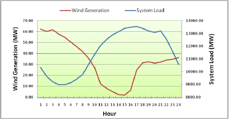
happens during peak load period. The worst scenario is that a wind project is sited where wind is rich at night during winter season, meanwhile, system load peak takes place in daytime during summer season. Figure 1-3 shows an area load profile and an aggregated wind generation of several wind farms for 24 hours in a day in the western region. It is obvious that the trends of load shape and wind generation deviate from each other.
Figure 1-3 Unfavorable daily wind generation pattern
1.3. Impact of Wind Power on Power System Planning and
Operation
In power system operations, the main goal is to ensure the reliability of an electric power supply system which continuously faces anticipated and unanticipated changing conditions. Comprehensive processes of long-term planning and short-term operation are carried out to resolve the issues in the time frame from multiple years to milliseconds. In a traditional power system, operator dominates all available controllable resources to reliably serve the
primary independent uncontrollable variable, system load. Wind generation, as an undispatchable generating resource, almost entirely relies on wind availability. Integration of wind generation into existing power systems will definitely impact system planning and operation process in all time frames.
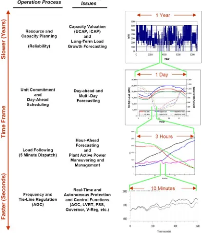
Figure 1-4 illustrates the time frames from long term to short term for planning and operation [3]. Investigation of wind generation integration must be carefully performed to accommodate to system’s needs for different time frames.
♦ In the long-term planning time frame, expansion decision of system infrastructure including resource and transmission are made with looking several years ahead to meet demand growth and satisfy reliability requirement. Wind generation, depending on geographical location and climatic condition, varies a lot from season to season and from year to year. Development of wind generation needs collaborate with generation and transmission planning, especially for the conventional generating units, to satisfy resource adequacy.
♦ During day-to-day scheduling, available generating resources are scheduled beforehand based on the predicted upcoming load demand and wind generation, as well as other system conditions, such as transmission constraints and maintenances. Not like system load that conforms to diurnal cycle, availability of wind is largely unpredictable. To some extent, forecast error of wind generation is much greater than that of load, particularly for mid-term and long-term forecast. Logic of unit commitment considering operation reserve requirement needs be adjusted under high wind penetration condition.
♦ During an operation day, also known as real-time operation, economic dispatch determines the minute-to-minute generation from the generating units that are committed based on unit commitment decision in the past, typically previous day. Unit commitment is potentially refined to accommodate the deviation between the forecast and actual value of load and wind generation and any other types of contingencies.
♦ In the fastest time frame, minute to second level, generating facilities are handled by automatic generation control and governor action without much operator intervention in response to system variations to meet system frequency and scheduled interchange among control areas. Large and high frequency variations of wind generation barely happen in such short period. Therefore, impact in this time frame is relatively small and could be negligible.
Figure 1-4 Time frames for power systems planning and operation
1.4. Wind Generation Integration Issues
Intermittence, uncontrollability, poor predictability and unfavorable seasonal and daily pattern in nature of wind generation raise a series of issues to power systems whether load demand can be continuously reliably served in terms of the influence of wind generation in all stages of planning and operation.
♦ How does the system reliability change when individual wind project is integrated in a system to reach different penetration level? Is the existing power system able to maintain the reliability requirement when high wind power penetration happens?
♦ What is the optimal development order of a wind project queue, which can improve system reliability?
♦ How does the performance of wind generation forecast affect scheduling and operation as well as the overall system reliability?
♦ How does the traditional resource planning cooperate with wind generation to create a desirable generation mix to meet future load demand?
♦ Besides the anticipatory contingencies in an existing system, is current operation reserve able to cover uncertainty of wind generation? How to determine the operational reserve requirement under certain level of wind penetration?
♦ Is wind generation qualified for capacity value? If so, how to quantify the appropriate amount for individual wind project?
♦ Should traditional system operating practices including unit commitment and economic dispatch be changed in respond to intermittent wind generation?
♦ Should power market rules be adjusted to accommodate the nondispatchable nature of wind generation, and maintain a fair and competitive market?
♦ How does the utilization of different types of conventional generating unit change?
♦ How do overall system production cost, generation revenue and load payment change? Is there any additional integration cost for wind generation due to the unfavorable behaviors?
About a decade ago, installed capacity of wind generation was just a very small portion among the entire generating resources in bulk power systems and the effects on system reliability could be negligible. Along with large-scale wind power penetration into bulk power systems, the amount of wind power generation is comparable to the amount of existing conventional generating resources. Power systems primarily emphasize on providing a reliable and economic supply of electrical energy to customers. New methods for system planning and operation need to be introduced due to the significant impacts of wind intermittence on operating conventional generation resource. Especially, in the impartially competitive electric markets, Independent System Operator (ISO) and Regional Transmission Organization (RTO) have to deeply understand and investigate technical and economic impacts of wind power on deregulated power systems so that reasonable market regulations specifically for wind power can be established.
1.5. Thesis
Overview
In order to address some of the issues regarding integration of wind power, a Monte Carlo based production cost simulation model has been investigated. The model simulates realistic processes of system planning and operation and takes wind generation into account. The main objective of the proposed model is to evaluate reliability of a power system integrated with wind generation. It also can be used for estimating the effects of wind generation forecasting, system reserve requirement, capacity value of a wind project, and so on.
Chapter 2 presents the concepts of power system reliability and its evaluation methods. There are basically two main branches for reliability evaluation, analytical based method and Monte Carlo simulation method. Typical power system operation process including day-ahead scheduling and real-time operation is also described in this chapter.
Chapter 3 mainly focuses on wind generation related topics. Firstly, the fundamentals of wind generation are introduced. In addition, the applications and state-of-the-art methodologies of wind power forecasting are simple reviewed. At the end, the basic concept of capacity value of wind power is discussed.
Chapter 4 proposed a Monte Carlo based production cost simulation model that mainly will be applied for reliability evaluation of power systems with wind power integration. In the model, there are three major iteration loops including, Monte Carlo replication loop, daily loop and hourly loop. Actual system operation processes considering wind generation, such as day-ahead unit commitment and real-time refinement are mimicked. A simplified unit commitment method is adopted to fit the simulation for reliability evaluation purpose. An automatic process for day-ahead hourly wind generation forecasting is proposed as well using Auto-Regressive Moving Average (ARMA) model. The forecasted and actual values of wind generation are applied for day-ahead and real-time scheduling, respectively. At the end, the IEEE Reliability Test System (RTS) is simulated using the proposed model to verify its feasibility and validity. Results show that the reliability indices reported from the proposed model is reasonably close to the one calculated by analytical method.
Chapter 5 is a case study using the proposed Monte Carlo simulation model. A power system as a base case with a desired generation mix is created based on the data from real power systems. The annual hourly generation profiles of four wind projects are prepared. The study shows that power system reliability as well as system economics and generation utilization are indeed highly impacted by wind generation integration. The importance of wind forecast performance is also proven by simulation results. Capacity value of a wind project is assessed using different methods.
Chapter 6 concludes the thesis and suggests the future works to further improve the Monte Carlo simulation model.
1.6. Abbreviations
♦ NERC: North American Electric Reliability Corporation
♦ LOLE: Loss of Load Expectation
♦ EENS: Expected Energy Not Served
♦ WTGS: Wind Turbine Generator System
♦ ISO: Independent System Operator
♦ RTO: Regional Transmission Organization
♦ ARMA: Auto-Regressive Moving Average
♦ RMSE: Root Mean Square Error
♦ FOR: Forced Outage Rate
♦ MTTR: Mean Time To Repair
♦ MTTF: Mean Time To Failure
♦ ELCC: Effective Load Carrying Capability
Chapter 2
Power System Reliability
2.1. Concept of Power System Reliability
Reliability is the probability of a device performing its purpose adequately for the period of time intended under the operating conditions encountered [4]. Bulk power system reliability has two aspects, each requiring its own set of criteria and system testing procedures. NERC defines reliability as follows [5].
♦ Adequacy - The ability of the bulk power system to supply the aggregate electrical demand and energy requirements of the customers at all times, taking into account scheduled and reasonably expected unscheduled outages of system elements.
♦ Security - The ability of the bulk power system to withstand sudden disturbances such as electric short circuits or unanticipated loss of system elements from credible contingencies. With a set of operating and design criteria to ensure system secure operations and system stress level before any credible contingency under various operating conditions and active and reactive power reserves on the system plays a major role in deciding the generation dispatches.
Adequacy and security are considered the basic inputs to the generation side of system reliability. In despite of distinct concepts, they are closely correlated. A system with adequate capacity can maintain enough security to reduce periods of involuntary load shedding [6]. Regarding adequacy, system operators can and should take controlled actions or procedures to maintain a continual balance between supply and demand within a balancing area. A system is adequate if the probability of having sufficient transmission and generation
to meet expected demand is equal to or less than the system’s standard. Two main components affect adequacy are generation system and transmission system.
The methods for assessing generating resource adequacy can be categorized as deterministic methods and probabilistic methods. Capacity margin, a typical deterministic metric, is the amount by which capacity exceeds system peak demand expressed as percent of capacity resources. Probabilistic method is associated with an evaluation that explicitly accounts for the likelihood and consequences of possible contingencies sequences in an integrated fashion and provide the expected reliability indices. Power systems frequently experience random disturbances such as outage of generator or loss of transmission line, so-called contingencies. Therefore, it is logical to assess such system using probabilistic techniques. The essence of probabilistic based adequacy can be accounted by load curtailment measures (e.g., LOLE) that estimates the minimum amount of load that needs to be curtailed to avoid unacceptable system problems following contingencies and utilizing all available system adjustments. The commonly accepted quantitative indices of reliability assessment are Loss of Load Expectation (LOLE), Loss of Load Probability (LOLP) and Expect Energy Not Served (EENS).
2.2. Reliability Evaluation Methodology
Power system reliability can be estimated using a variety of methods. There are basically two main approaches for power system reliability evaluation that are widely accepted in the industry, analytical based method and Monte Carlo simulation based method [7]. Either of them is able to compute reliability indices. In the thesis, reliability methods mainly focus on assessing generation adequacy.
2.2.1. Analytical Method
Analytical techniques assess system reliability using direct numerical solutions. The expected risk of loss of load is calculated using applicable system capacity outage probability table combined with the system load characteristic.
The basic generating unit model used in reliability evaluation is a two-state model that represents the probability of finding the unit on forced outage at some distant time in the future. The probability is defined as the unit unavailability, and historically in power system applications it is known as unit Forced Outage Rate (FOR). The concepts of the availability and unavailability are illustrated in Equation (1) and Equation (2).
( ) r DownTime
Unavailability FOR U
m r DownTime UpTime
= = =
+
∑
∑
+∑
(1)UpTime m
Availability A
m r DownTime UpTime
= = =
+
∑
∑
+∑
(2)where, m is Mean Time To Failure (MTTF), r is Mean Time To Repair (MTTR) and m+r is Mean Time Between Failures (MTBF).
FOR in equation is associated with the two-state outage model, in Figure 2-1, that can be directly applicable to a generating unit which is either operating or forced out of service. In Figure 2-1, λ is the expected failure rate, as in Equation (3), and μ is expected repair rate, as in Equation (4).
Unit Up Unit Down
λ
µ
Figure 2-1 Two-state model of a unit availability
1
MTTF
λ = (3)
1
MTTR
μ = (4)
Capacity outage probability table tabulates total available generating capacity amounts and their associated probabilities. It is created based on installed capacity and unavailability probability of each individual generating unit in the system. The basic probability concept can be applied to calculate the probabilities of different availability status combinations of all generators.
In an example system, there are two 3 MW units and one 5 MW unit. All their FOR are 0.02. The capacity outage table is listed in Table 2-1. For instance, there are two situations will lead to total out of service capacity of 3 MW. One is the first 3 MW units and the 5 MW unit are in service and the second 3 MW is out of service. Another one is the second 3 MW units and the 5 MW unit are in service and the first 3 MW is out of service. Its probability can be found in Equation (5), assuming the service status of each unit is an independent event.
Table 2-1 Capacity outage probability table
Capacity out of service (MW) Individual probability Cumulative probability
0 0.941129 1.000000
3 0.038416 0.058808
5 0.019208 0.020392
6 0.000392 0.001184
8 0.000784 0.000792
11 0.000008 0.000008
0.02*(1 0.02)*(1 0.02) 0.02*(1 0.02)*(1 0.02)
Probability= − − + − − (5)
In realistic systems, the number of units is huge. Exhaustively enumerating the service status combinations of all units is not feasible in terms of the large computation efforts. Techniques have been developed to create capacity outage table for real systems. More details can be found in [7].
Reliability indices can be mathematically calculated with combining system load profile and capacity outage probability table. LOLE can be measured by different period, such as hours/year, days/year or hours/month. Equation (6) shows LOLE calculation. If an annual
system load is provided on hourly basis, in the equation, N is the total number of hours in a year. LOLE is the accumulated value of loss of load probability at each hour. Probability of loss of load at individual hour can be directly obtained from the capacity outage probability table.
1
(
N
i i i
i
LOLE P C L
=
=
∑
− ) (6)where, Ciis total capacity in system at hour i, is system load at hour i, and Li P Ci( i−Li)is
the probability of loss of load at hour i.
Analytical method generally provides expectation reliability indices in a relatively short computing time. It relies on capacity outage table that tells the exact probability of each level of outage capacity. However, building capacity outage table for the real power systems is much more complicated due to the huge amount of outage combinations among generators in the system.
2.2.2. Monte Carlo Simulation Based Method
Monte Carlo methods are a class of computational algorithms that rely on repeated random sampling to compute the statistics. More broadly, Monte Carlo methods are useful for modeling phenomena with significant uncertainty in the systems. It is used for obtaining numerical solutions to problems which are too complicated to solve analytically. In an analytical method, unfortunately, assumptions are frequently required in order to simplify the problems. The resulting analysis possibly fails to catch its significance. Particularly, when complex systems and complex operating procedures have to be considered, analytical method is not even capable to achieve the correct solution. Therefore, the simulation techniques are very important in the reliability evaluation in such situation. In the past, the majority techniques for reliability evaluation are analytical based methods. Nowadays, especially after the booming of power markets, Monte Carlo simulation is increasingly considered by system
planner due to the capability of modeling system behavior more comprehensively and informatively. Sequential Monte Carlo method is typically applied for solving the uncertainty of a system in chronological order. If the operating life of the system is sufficiently simulated using Monte Carlo method, it is possible to conclude the behavior of the system and obtain a clear picture of the type of deficiencies that the system may suffer.
Monte Carlo simulation methods estimate power system reliability indices by simulating the actual operations and random events in the system. The method treats the problem as a series of real experiments. The techniques can take into account virtually all aspects and contingencies inherent in the operation of a power system. The goal of Monte Carlo simulation is to achieve the statistics of the realistic system by making a large amount of trials for the happening in the system. This recorded information permits the expected values of reliability indices together with their frequency distributions to be evaluated. First of all, it is worthwhile to introduce the basic concepts of power system operations.
2.2.2.1. Power System Operations
A power system is an extremely large and complicated system that contains thousand of individual components. The most important goal in power system operation and planning is to continually provide reliable electric energy to customers. Meanwhile, the system must optimize the available resources to minimize the total system production cost subject to all kinds of constraints.
In Unites States, besides the traditional vertically-integrated utilities, power markets are established all over the places. ISO and RTO are not-for-profit corporations that ensure the reliability of electric power supply systems, operate and administer wholesale electricity markets and manage the regional electric resource and transmission planning for its control area. The existing power markets in Unite States include:
♦ Pennsylvania New Jersey Maryland Interconnection (PJM RTO)
♦ New York ISO (NYISO)
♦ ISO New England (ISO-NE)
♦ California ISO (CAISO)
♦ Midwest ISO (MISO)
♦ Southwest Power Pool (SPP)
♦ Electric Reliability Council of Texas (ERCOT)
A control area overseen by ISO consists of generating units, load and transmission facilities that are owned by market participants. An ISO optimizes the available resources to minimize the total system production cost subject to all kinds of constraints. Typically, in a power market, the operating activities are broken down into two settlement systems and performed on continuously basis. The simple description of the two settlement systems, day-ahead market and real-time market, can be found as follows.
In day-ahead market, the basic information needs to be collected from market participants for the following day scheduling are load forecasting, renewable generation forecast, generator bid cost and load purchase offer. System operators will perform least cost Security Constraint Unit Commitment (SCUC) to determine the next day hourly schedule of generators considering all system constraints.
In real-time market, system operators make any necessary refinement for generating resources to closely serve actual system load during the day of operation by performing least cost Security Constraint Economic Dispatch (SCED) for every five minutes. The real-time system conditions could deviate from the forecasted value and incur unexpected contingencies. Random events, such as generator forced outage, may happen any time during operation.
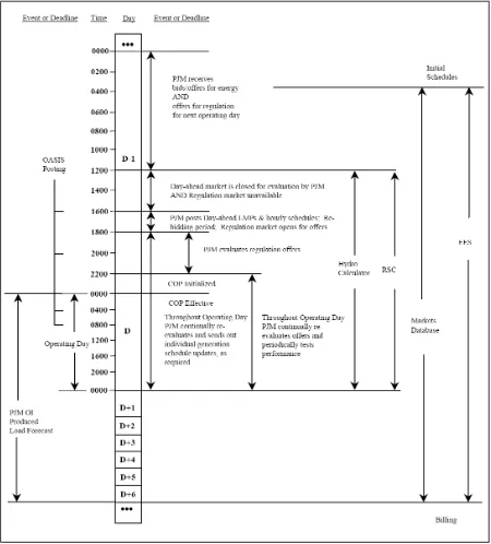
The operation activities in the form of a time line that is referred from scheduling operation manual of PJM market is shown in Figure 2-2 [8]. The reference point of the timeline is the operating day. Specific detailed operation rules can be found in different power markets.
Figure 2-2 Scheduling timeline
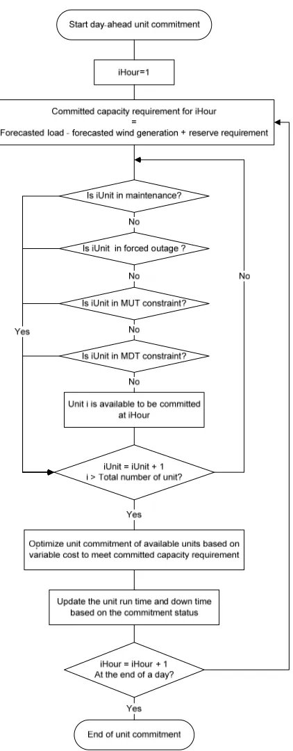
2.2.2.2. Unit Commitment
Among the operation procedures, unit commitment is very critical. Firstly, it decides the available capacity to be dispatched for load serving during real time. Secondly, it affects overall system economic efficiency. Meanwhile, it has to take system uncertainties into account so that sufficient capacity is available for maintaining system reliability. Unit commitment problem can be defined as the production scheduling of electric power generating units over certain time horizon. Meanwhile, the problem solution must respect both generator physical constraints and system operational constraints. The key outcomes determine each generating unit’s hourly status that is to either be committed online, namely, synchronized with system or stay offline. Unit commitment is essentially an optimization problem that can be mathematically represented by Equation (7) to Equation (14) in which each generator is marked by unit index i and hour number t.
, , ,
it it it
i t i t i t
Minimize
∑
FixedCost +∑
GenerationCost +∑
StartupCost (7)subject to,
it t
i
TotalGeneration =Load
∑
(8)it t
i
SpinningReserve =SpinningReserveRequirement
∑
(9)i it i
MinimumCapacity ≤Generation ≤MaximumCapacity (10)
MinimumUpTime Constraint (11) MinimumDownTime Constraint (12)
Ramping Constraint (13)
Transmission System Constraint (14)
The objective function of the optimization is to minimize the total system production cost that contains:
♦ Fixed cost is a constant cost whenever the generator is committed and not associated with generation dispatch.
♦ Generation cost associated with dispatch amount of a generator typically includes fuel cost and Operation and Maintenance (O&M) cost.
♦ Startup cost is the cost for turning on a generator from offline status. Because the temperature and pressure of a thermal unit must be moved slowly, a certain amount of energy must be expended to bring the unit on-line. This energy does not result in any generation from the unit and it brought into the unit commitment problem as startup cost.
There are different kinds of constraints that make the optimization really complicated.
♦ Energy balance constraint makes sure total generation from committed generators meets system load for each hour.
♦ Operational spinning reserve as a part of ancillary services is to help maintain the security and the quality of electricity supply. Spinning reserve can be generally defined as the unused capacity which can be activated on decision of the system operator and which is provided by generating units which are synchronized to the network and able to affect the active power. Spinning reserve is a critical resource to respond to unforeseen events, such as unit forced outage, wind generation forecast error. Its requirement can be given by a fixed value based on the most serious contingency. Spinning reserve amount from qualified generators needs to satisfy system reserve requirement.
♦ Total output from each generator is limited by maximum and minimum capacity.
♦ Output from each generator for spinning reserve purpose is limited by maximum and minimum spinning reserve capacity.
♦ Minimum up time, also known as minimum run time, is the minimum number of hours of operation at or above the minimum generation. In another word, once the
unit is committed to generate power, it must stay online and can not be turned off for specific hours.
♦ Minimum down time is the minimum number of hours between the time the generator is shut down and the time the generator is re-committed to generate power.
♦ Ramping constraints restrict the deviation of individual generation dispatch between present hour and next hour in terms of ramp up rate and ramp down rate.
♦ Transmission constraints honor the limitation of the transfer capability of transmission systems, such as thermal rating of individual transmission line, contingency constraint, flow gate constraint, etc.
Unit commitment could be a large-scale and very complicated optimization problem according to the size of system, required constraints and the level of model details. Unit commitment can be solved by various optimization methods, such as priority-list schemes, Dynamic Programming (DP), Mixed Integer Programming (MIP) and so on. MIP is able to very well represent unit commitment. Term “Integer” in MIP appropriately represents the binary variable for the hourly commitment status of a generator. One MIP may determine the hourly generator scheduling for certain period in terms of the planning needs, for example, one day or one week. Therefore, the number of the integer variables for hourly commitment status of individual generator is the total number of hour in the optimization period. Nevertheless, due to the solving difficulty, MIP is still under investigation and improvement. The latest research of unit commitment is detailed in [9].
2.2.2.3. Reliability Assessment
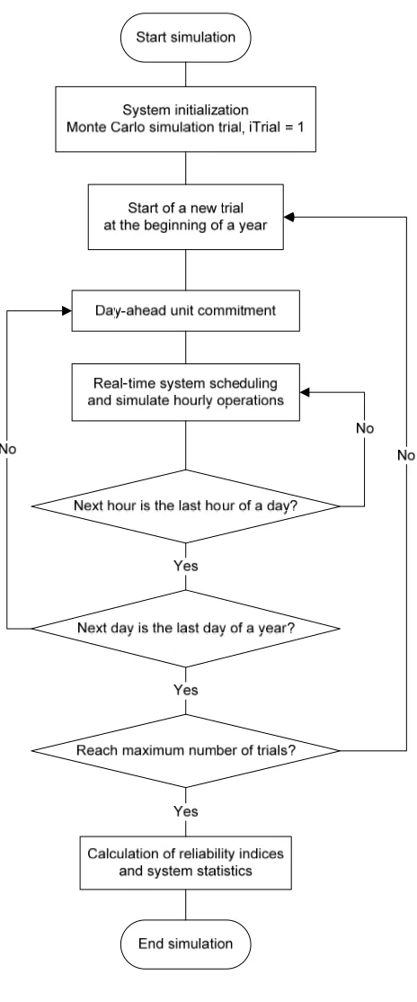
Reliability evaluation using Monte Carlo simulation requires significant amount of calculation effort. The expect value of the statistics based on the simulation results is achieved by largely replicating realistic system planning and operation processes during specific period. Chronological load profile needs to be prepared. A typical procedure is consisted of the following steps.
1. Simulation starts typically at the beginning of a year.
2. Perform day-ahead unit commitment.
3. Perform real-time operation by economic dispatch based on generator availability and load profile. Meanwhile, system random behaviors, such as generator forced outage, are modeled.
4. Repeat step 2 and step 3 until the end of the year.
5. Count the annual number of hours at which the total available generating capacity is not enough to serve the corresponding load. Sum up the amount of unserved load for all hours, if any, to get total unserved load in MW for the whole year.
6. Repeat step 1 to 5 until the stop criterion, such as the maximum number of replication, is reached.
After plentiful replications of system operation for the same period, statistic expectation of any system performance is computed. Calculation of reliability indices LOLE and EENS can be found in Equation (15) and Equation (16), where N is the total number of trials and y is the trial number.
1
( /
N
y y
Total Hours of Loss of Load
)
LOLE Hours Year
N
=
=
∑
(15)1
( /
N
y y
Total Amount of Loss of Load
)
EENS MWh Year
N
=
=
∑
(16)Chapter 3
Wind Power Generation Fundamentals
3.1. Wind Power Production
The kinetic energy per unit time, or power, from wind is given by Equation (1) [10]. Wind power is proportional to the cube of the wind velocity.
3
1
* * * 2
Power of Wind = ρ A V (1)
where, P is power in watts, ρis air density in kg/m3, A is area exposed to the wind (m2), and V
is wind speed in m/s.
The actual power production potential of a wind turbine must take into account the fluid mechanics of the flow passing through a power producing rotor, the aerodynamics and efficiency of the combination of rotor and generator. In practice, a maximum of about 45% of the available wind energy is harvested by the best modern wind turbines. Power output from wind turbine can be seen in Equation (2).
3
1
2 p
Wind Turbine Power Output = ∗ ∗ ∗ρ A C ∗V ∗Ng Nb∗ (2)
where, P is power in watts, ρis air density in kg/m3, A is area exposed to the wind (m2), V is
wind speed in m/s, is performance coefficient (Maximum 0.59), Ng is generator
efficiency (80% on average for grid-connected induction generators), and Nb is gearbox and bearings efficiency (Maximum 95%).
p C
The power produced by a wind turbine can be shown by a power curve. The power curve of a wind turbine is a function that indicates how large the electrical power output will approximately be for the turbine at different wind speeds. The power curve illustrates three important characteristic velocities:
♦ Rated wind speed: the wind speed at which the rated power of a wind turbine, generally the maximum power output of a generator at highest efficiency, is produced.
♦ Cut-in wind speed: the minimum wind speed at which a generator starts delivering power.
♦ Cut-out wind speed: the maximum wind speed at which the turbine is allowed to produce power, usually limited by engineering design and safety constraints. No power will be produced by a wind turbine beyond the cut-out speed.
Figure 3-1 shows the power curve of GE 3.6 MW offshore series wind turbine, where rated speed is 14 m/s, cut-in speed is 3.5 m/s and cut-out speed is 27 m/s.
Figure 3-1 Power curve of GE 3.6 MW offshore wind turbine
A group of wind turbines at the same location are interconnected with a medium voltage power collection system and communication networks, which forms a wind farm. Figure 3-2 shows a typical configuration of a wind farm. The power generated from individual turbine
are aggregated and delivered to major power systems from the substation at wind farm through transmission systems. A wind farm may be located offshore to take advantage of strong and steady winds blowing over the surface of an ocean or lake.
Figure 3-2 Wind farm configuration
3.2. Impacts on Power Systems
In chapter one, the favorable and unfavorable features of wind generation are described. Even though wind generation brings various benefits to power system, it introduces challenges to electric grids due to its unpredictability, intermittence and high fluctuation. Wind generation, as an uncontrollable generating resource, will impact power system long-term planning and short-long-term operation process.
During operation scheduling stage, system operators assume to employ the best forecasted wind generation for making commitment decision of conventional generators. Certain amount of capacity including energy and reserve requirement will be committed online at designated time to server upcoming, typically next day, load demand. While it is very
difficult to accurately forecast wind generation and no perfect wind forecasts are guaranteed. Consequentially, difference between forecasted and actual amount of wind generation will raise issues for system reliability and extra operating cost during operating hours. There are two scenarios can be expected.
3.2.1. Under forecast of wind generation
The day-ahead forecasted value is less than the real-time actual value, which possibly leads to over-commitment. If capacity is over-committed, some units might need to reduce dispatch at real time. If capacity is too much over-committed, consequently, the total minimum capacity of all the committed generators is greater than the actual net load that is difference between actual load and actual wind generation. In order to maintain operation feasibility, some generators have to be shut down or wind generation is curtailed. The reason of this is that the forecast of wind generation is much low than the actual wind generation. Unnecessary startup or shutting down will incur additional operating cost. However, under forecast of wind generation will normally not jeopardize system reliability.
3.2.2. Over Forecast of Wind Generation
The day-ahead forecasted value is greater than the real-time actual value. In this scenario, committed capacity, as well as the import power from outside of the system, which are scheduled during day-ahead unit commitment, may not be able to entirely meet the real-time net load. Typically, operation reserve will pick up a small amount of generation deficiency. If operation reserve is not enough to deal with such emergency, in result, during real-time dispatch, more expensive units including quick start units must be immediately fired up to recover the capacity shortage, which will also cause energy price rising. If available units are not quick enough to respond, load shedding will happen.
Wind characterizes volatility and unpredictability, so does wind generation. Moreover, the fast ramping up and down is hard to be captured by day-ahead hourly forecast and large forecast error between day-ahead forecast and the actual value at present hour is expected.
Figure 3-3 shows the historical hourly generation of wind farm Prince in Canada on September 7th, 2007. It is obviously to see the fast ramping up and down in the plot. Wind generation suddenly drops 92 MW from 2pm to 3pm and bumps up 108 MW from 4pm to 5pm. These features of wind generation will make difficulties for system operation and forecast, particularly, when high wind penetration happens in bulk power systems.
Figure 3-3 Fast ramp up and down of wind generation
From the analysis of the impacts by wind generation, on the one hand, the system may incur additional operating cost due to the adjustment of operation scheduling. On the other hand, more seriously, system reliability is potentially endangered due to the unfavorable features of wind generation that may create operation difficulties. Actions, such as adjustment of spinning reserve requirement, preparation of more quick start units, must be taken when high penetration of wind generation occurs in power systems.
3.3. Wind Energy Forecasting
One of the most important prerequisites for effective wind power planning and operation in bulk power systems is the precise wind power and speed forecasting. Highly random
fluctuation of wind affected by conditions of atmosphere, weather and terrain results in the difficulties of forecasting and it happens on all time scales from short-term to long-term. In comparison with load daily, weekly and seasonal patterns, there are much less patterns of wind can be obeyed. Therefore, wind generation is considered as one of the most difficult predictable variables [11]. Wind power forecasting were investigated over the decades, some researches can be seen in [12], [13], [14], [15], [16], [17] and [18].
Basic economic operating functions such as unit commitment, interchange evaluation and security assessment require a reliable and accurate wind power forecasting. The applications of wind power forecasts over a varying period of time include following items:
♦ Very short-term wind forecast from seconds to minutes is applied for wind turbine control systems that include yaw orientation and blades rotation.
♦ For the optimization of conventional power plants scheduling, such as economic dispatch, prediction horizons can vary from minutes to several hours depending on the size of the system and the types of conventional units.
♦ In day-ahead market, predictions looking ahead from 1 hour to 48 hours are required by different types of end-users for different functions such as unit commitment, dynamic security assessment for operators, bidding strategies for market participants in the power market.
♦ Longer time scales would be interested by maintenance planning of large power plants, wind turbines or transmission systems. However, the accuracy of weather predictions decreases strongly looking at 5-7 days in advance.
♦ Long-term wind forecasts is used for development planning of wind power generation, as well as power system planning with integration of wind generation.
3.3.1. Importance of Wind Forecasting
Accurate wind power forecasts are beneficial for wind plant operators, utility operators, and utility customers. An accurate forecast allows grid operators to schedule generation economically and efficiently to meet demand of electrical customers. In particular, under
deregulated power market environment, reliable long-term wind power forecast is beneficial for system resource and transmission planning to ensure the generation adequacy. Furthermore, as the must-taken energy, wind generation plays a very important role by straightly impacting SCUC and SCED, reserve requirement and market clearing price in day-ahead and real-time market. System operators will be benefit from accurate short-term wind forecasting by economically scheduling generation to reliably serve the load.
3.3.2. Wind Forecasting Methodology
Persistence forecasting model, also called naive method, is the most frequently used model. It is the simplest forecasting models. In this model, forecast for all times ahead is set to be the value as present value, in another word, wind speed at time t + x is the same as it was at time t. For short-term forecast, persistence model performs very well for up to 3 hours ahead forecast. The accuracy of this forecasting method quick reduces when increasing x. Therefore, by definition, error for zero time steps ahead is zero. For short prediction horizons (seconds, minutes to hours level), this model is the benchmark all other prediction models have to beat. The common used criteria to evaluate the performance of wind power forecasting are listed below. They are computed by comparing wind power forecasts with historical data or persistent model forecast results.
♦ Root Mean Square Error (RMSE)
♦ Mean Absolute Error (MAE)
♦ Median Error (ME)
♦ Frequency distribution of error
Short-term wind power forecasting is used for wind turbine controls, real-time dispatch or generation scheduling depending on the time scale of specific purpose. In general, forecasting methods can be broken down into two main categories or their combination.
♦ Physical model considers Numerical Weather Prediction (NWP), detailed conditions of wind farms and their surrounding terrain. It reaches the best possible estimation of the local wind speed and reduces the remaining error.
♦ Statistical time-series related methods include Auto-Regressive Moving Average (ARMA) [12], [13], Artificial Neural Networks (ANN) [14], [15], Fuzzy Logic [16], Kalman Filter, and so on. Statistical models catch the relationships between variables including NWP results and online measured data and usually employ recursive techniques. Prediction capabilities and accuracy of the models or their combination are quite different in terms of forecasting interval. The overview of short-term wind power forecasting methodologies and their corresponding performance can be found in [17]. Typical input and output data of commercial wind power forecasting tool can be found in Figure 3-4.
Figure 3-4 Structure of commercial wind power forecasting tool
Long-term wind forecasting typically scaled from several months to multiple years is applied to estimate overall wind resource condition, optimize wind turbines layout in a wind farm and determine the wind farm sites. A number of possible approaches including statistical method, computer modeling, wind atlas, ecological methods have been developed.
3.3.3. Time Series Models
One of the widely used time series models is Auto-Regressive Moving Average (ARMA). ARMA procedure analyzes and forecasts equally spaced univariate time series data, transfer function data, and intervention data. An ARMA model predicts a value in a response time series as a linear combination of its own past values, past errors and current and past values of other time series. The model is usually referred to as ARMA (p, q) model where p is the order of auto-regressive part and q is the order of the moving average part. Mathematical representation of ARMA (p, q) can be seen in Equation (3).
1 1
p q
t t i t i j t
i j
x ε ϕx− θ ε −j
= =
= +
∑
+∑
(3)where, (ϕi i=1, 2,..., )p are the parameters for Auto-Regressive (AR), (θj j=1, 2,..., )q are the
parameters for Moving Average (MA), and εt is a normal white noise process with zero
mean and a variance of 2
a
σ , namely, , 2
t N(0 a)
α ∈ σ .
An ARMA analysis is typically divided into three stages, corresponding to the stages described by Box and Jenkins [19].
1. Identification: In the identification stage, the response series will be specified. The pre-processing of the input time series includes basic statistics analysis, computation of autocorrelations, inverse autocorrelations, partial autocorrelations, and cross-correlations. Stationarity tests can be performed to determine if differencing is necessary. The orders of AR and MA will be tentatively determined.
2. Estimation: In the estimation and diagnostic checking stage, the parameters of ARMA model to fit to the variable specified in the previous stage will be estimated. Diagnostic statistics can be produced to judge the adequacy of the model. Significance tests for parameter estimation indicate whether some terms in the model might be unnecessary. White noise tests for residuals indicate whether the residual
series contains additional information that might be used by a more complex model. If the diagnostic tests indicate problems with the model, another model will be estimated and then repeat the estimation and diagnostic checking stage.
3. Forecasting: In the forecasting stage, future values of the time series will be forecasted based on the selected ARMA model from previous stage and confidence intervals for these forecasts from the ARMA model will be generated as well.
3.4. Capacity Value of Wind Power
Wind generation brings a great amount of benefit to power systems, such as cheap energy, emission reduction, power provision for remote areas, etc. However, whether a WTGS can be assigned any capacity credit is controversial among power markets and utilities. If so, how much appropriate capacity credit can be assigned?
Capacity value of a wind generating system must be careful decided. In order to ensure electric supply reliability, ISO and RTO as well as utilities measure resource adequacy. When capacity value of wind generation is considered as part of generation planning process, system operators and planners are able to estimate conventional generation expansion in which the sites, timing and amount of new generation additions are determined. Accurately evaluating wind capacity value may stint the investments of new generation additions for the purpose of maintaining capacity reserve. When wind capacity value is underestimated, system may overpay for reliability by investing too much reserve capacity.
Capacity value of a WTGS can be paid in capacity markets. In a deregulated power market environment, wind generation is treated as the must-taken energy and is paid based on market clearing price and the amount of generation. According to different markets settlement rules, a WTGS will be charged for penalty cost if scheduled energy can not be delivered on time. The economic benefit of a WTGS can not be guaranteed all the time. In addition, subsidizing program and tax reduction are founded for the economic incentives for wind power development. A WTGS may receive revenue from capacity markets based on its capacity value. Generally speaking, in a locational capacity market, suppliers are paid based
on their demonstrated ability to supply energy or reserves in shortage hours in which there is a shortage of operating reserves. Thus, only supply that contributes to reliability is rewarded [20]. Revenue from capacity market is the supplement of WTGS’s revenue received from the energy and reserves markets.
3.4.1. Methodologies for Capacity Value Estimation of A WTGS
Capacity value of a WTGS is determined mainly by its impact on power system reliability and resource scheduling. In general, capacity value of a generating unit is not the nameplate capacity and primarily depends on the actual availability of generating capability during critical periods with high risks, such as system peak load period, which can be determined based on the installed capacity, force outage rate, maintenance requirement, fuel availability, and so on.
Because wind generators only generate electricity when wind blows, effective forced outage rate, namely, the probability of unavailability, for wind generators may be much higher than one of conventional generators when recognizing the intermittent, fluctuant availability of wind. In addition, capacity value of a WTGS to a specific electric system may also vary quite a bit. Generation from certain wind farms may highly positively correlate with system load and thereby can be seen as supplying capacity when it is most needed. In this situation, a wind generating plant should have a relatively high capacity credit. On the other hand, output from other wind generating plants could be out of phase with system load, and therefore a lower capacity value to the electric system should be assigned [21].
A metric evaluating capacity value needs recognize the probability of generating failure during critical period and reward a generating unit that experiences less outage more capacity credit than the one with more unavailability. The capacity value must therefore be a probabilistic-based metric that can take wind generation and system load profile into account. The way to assign capacity credit for a WTGS currently varies among power markets and utilities [22]. Basically, there are three methods to estimate the capacity value of a WTGS.
3.4.1.1. Effective Load Carrying Capability (ELCC)
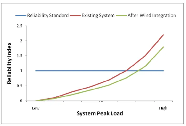
ELCC is deemed the prevalent metric of the capacity value of any generating unit. The very original concept of ELCC was developed in 1966 and can be found in [23]. Conceptually, ELCC is the additional load peak value that can be served with satisfying the same reliability standard of existing system after the integration of any new generating unit. It also can be applied to evaluate the capacity value for a wind generating system, such as a wind farm, that produces the energy aggregated from individual wind turbine. ELCC can be carried out by a power system reliability model. If yearly LOLE is measured for reliability index, Equation (4) shows the calculation of ELCC.
1 1 1
( , ) ( ,
N N M
i i j
i i j
LOLE C L LOLE C W L ELCC
= = =
= + +
∑
∑
∑
) (4)where, N is the number of existing generating units, is the capacity of unit i, L is annual
peak load, M is the number of additional wind farms, is the capacity of wind farm j.
i C
j W
The left hand side stands for the reliability value of existing system with N generating units. After integrating M wind farms into system, ELCC value can be found using the new system peak load when the reliability value in the right hand side is equal to the one in left hand side. Figure 3-5 more vividly explains the concept of ELCC. The blue line is assumed
the reliability criterionRc, for example, 1 day in ten years. ELCC is the difference part on the
blue curve between existing system and the new system with new wind generation.
Figure 3-5 ELCC illustration
3.4.1.2. Equivalent Conventional Generating Unit
The characteristics of the conventional generating units, such as thermal units and hydro units are well known. The method is to compare a WTGS with a conventional generating unit to server the same system load at same reliability level and take the capacity of the conventional generating unit as the capacity value of a WTGS.
Firstly, the existing power system is modeled without a WTGS. By using a reliability evaluation model, system load is adjusted to achieve a certain level of reliability requirement, for example, LOLE of one day in ten years. Once the desired LOLE target is achieved, the WTGS is integrated into the system and the system reliability is re-estimated. The new, lower LOLE (higher reliability) is noted, and the WTGS is removed from the system. Then the benchmark unit is added to the system by taking small incremental capacities until the LOLE with the benchmark unit matches the LOLE that was achieved with the WTGS. The capacity of the benchmark unit is then noted, and becomes the ELCC of the renewable generator. It is important to note that the ELCC documents the capacity that achieves the same risk level as would be achieved without the renewable generator.