Statistical Methods for Family-Based Association Studies for Complex Human Diseases: Single-Locus and Haplotype Methods

ABSTRACT

CHUNG, REN-HUA. Statistical Methods for Family-Based Association Studies for Complex Human Diseases: Single-Locus and Haplotype Methods. (Under the direction of Dr. Eden Martin.)

STATISTICAL METHODS FOR FAMILY-BASED ASSOCIATION STUDIES FOR COMPLEX HUMAN DISEASES: SINGLE-LOCUS AND HAPLOTYPE METHODS

by

REN-HUA CHUNG

A dissertation submitted to the Graduate Faculty of North Carolina State University

In partial fulfillment of the Requirements for the degree of

Doctor of Philosophy

BIOINFORMATICS

Raleigh, North Carolina 2006

APPROVED BY:

__________________________ ___________________________ Bruce S. Weir Eden R. Martin

Co-chair of Advisory Committee Co-chair of Advisory Committee

__________________________ ___________________________ Trudy F.C. Mackay Dahlia M. Nielsen

To my parents,

Biography

Acknowledgement

I am very grateful for the advice of my advisor, Eden Martin, during my doctoral studies. She is always patient and provides very helpful suggestions for the problems I encounter during my research. I always feel lucky and am proud of working with her. I also thank Dr Bruce Weir for his comments on my research and advice about course selection. I also would like to thank my other committee, Trudy Mackay, Dahlia Nielsen, Jung-Ying Tzeng, and also the graduate school representative, David McAllister.

I would like to thank the staff at the Bioinformatics Research Center, especially Juliebeth Briseno, who answered so many questions I had about graduate school regulations. I also thank Elizabeth Hauser, Richard Morris and Yi-Ju Li at Center for Human Genetics at Duke University for their advice and comments on my research. I also appreciate the support from members at CHG for testing and suggestions for the computer programs I have written.

I would like to express my special thanks to Ying-Erh Chen, who supports me with love and sincerity.

Table of Contents

List of Tables ... viii

List of Figures... ix

1 Review ... 1

1.1 Introduction to disease-gene mapping ... 2

1.2 Linkage analysis... 5

1.3 Association analysis... 6

1.3.1 Population-based association analysis ... 7

1.3.2 Family-based association analysis ... 9

1.3.3 Association in the Presence of Linkage method ... 13

1.4 X-linked analysis ... 16

1.5 Correlation between linkage and association analyses ... 20

1.6 Conclusion ... 23

2 The APL Test: Extension to General Nuclear Families and Haplotypes

and Examination of Its Robustness... 25

2.1 Abstract ... 26

2.2 Introduction... 26

2.3 Methods... 29

2.3.1 Review of the APL model... 29

2.3.2 Variance estimation ... 32

2.3.3 Extension to three affected siblings ... 33

2.3.4 Extension to multiple-marker haplotype analysis... 34

2.3.5 Rare alleles and rare haplotypes ... 36

2.3.6 HWE assumption ... 37

2.3.7 Computer simulations ... 37

2.4 Results... 39

2.5 Discussion ... 44

2.6 Acknowledgements... 47

2.7 Tables... 48

2.8 Figures... 55

3 X-APL: An Improved Family-Based Test of Association for the X

Chromosome... 58

3.1 Abstract ... 59

3.2 Introduction... 60

3.3 Methods... 63

3.3.1 X-APL statistic... 63

3.3.2 Variance estimation ... 66

3.3.3 Separate tests for males and females ... 67

3.3.4 Extension to multiple-marker haplotype analysis... 68

3.3.5 Hardy-Weinberg equilibrium assumption... 69

3.3.6 Computer simulations ... 70

3.4 Results... 73

3.4.1 Type I error and power ... 73

3.4.2 HWE effect ... 77

3.4.3 MAO genes for Parkinson disease... 78

3.5 Discussion ... 79

3.6 Acknowledgements... 84

3.7 Tables... 85

3.8 Figures... 93

4 Interpretation of simultaneous linkage and family-based association

tests in genome screens ... 95

4.1 Abstract ... 96

4.3.3 Incomplete pedigrees ... 103

4.4 Results... 105

4.4.1 Affected Sib Pairs with Parents ... 105

4.4.2 Extended pedigrees ... 109

4.4.3 Incomplete pedigrees ... 110

4.5 Discussion ... 111

4.6 Acknowledgement ... 114

4.7 Tables... 115

4.8 Figures... 120

5 Conclusions... 121

List of Tables

Table 2.1 Association configurations in SIMLA for the power simulations for haplotype tests.

... 48

Table 2.2 Mean, Variance and Type I error of the single-marker APL test across 5000 replicate data sets. ... 49

Table 2.3 Type I error of the multiple-marker haplotype APL global test across 5000 replicate data sets. ... 50

Table 2.4 Type I error of the single-marker APL test before and after the adjustment. ... 51

Table 2.5 Type I error of the multiple-marker haplotype APL test before and after the adjustment. ... 53

Table 2.6 Type I error of APL tests with HWE deviations... 54

Table 3.1 Genetic models used in simulations... 85

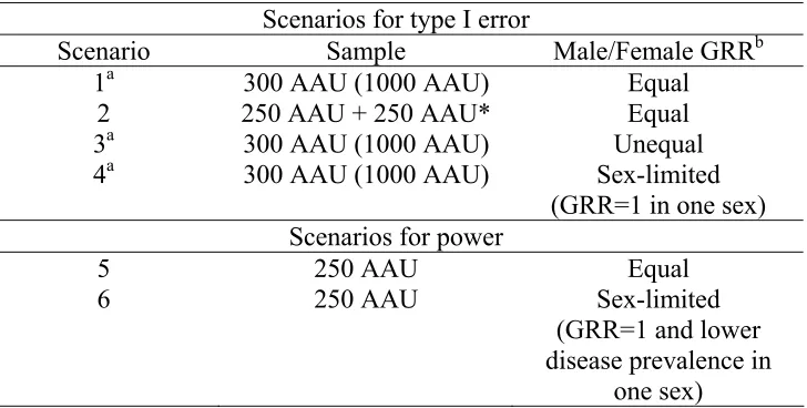
Table 3.2 Scenarios simulated for different family structures and genetic effects. ... 86

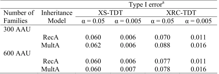
Table 3.3 Type I error of XRC-TDT and XS-TDT for 5000 simulated data sets... 87

Table 3.4 Type I error of XMCPDT for 5000 simulated data sets... 88

Table 3.5 Type I error of the X-APL tests for 5000 simulated data sets. ... 89

Table 3.6 Power estimates for X-APL test using all data and separate tests for males and females. ... 90

Table 3.7 Type I error of X-APL tests with HWE deviations... 91

Table 3.8 XS-TDT, XPDT, and X-APL results for MAOB gene analysis ... 92

Table 4.1 Parameters for simulated data. ... 115

Table 4.2 Correlation coefficient between MERLIN and PDT statistics... 116

Table 4.3 Type I error rates for PDT given a significant MERLIN test and MERLIN given a significant PDT. ... 117

Table 4.4 Correlation coefficient between MERLIN and APL statistics... 118

List of Figures

Figure 2.1 Power comparison for single-marker analysis... 55

Figure 2.2 Power comparison for haplotype analysis ... 57

Figure 3.1 Power comparison for single-marker analysis... 93

Chapter 1

1.1 Introduction to disease-gene mapping

In 1865, the Bohemian monk Gregor Mendel published “Experiments of Plant Hybridyzation,” which later became Mendel’s law of inheritance, and this law turned into an essential chapter in today’s genetics textbooks. Mendel studied traits that were mainly caused by segregation of a single gene. Thus, diseases caused by mutations in one gene are referred to as Mendelian diseases. Finding disease susceptibility genes is one of the major tasks in human genetics studies. Disease-gene mapping has been fairly successful for Mendelian disorders, mainly by the process of positional cloning [Risch, 2000]. Traditionally, genes were isolated based on the amino acid sequences of known proteins. Positional cloning has the property that genes are identified and mapped solely based on the inherited traits and no biological knowledge regarding the traits is required [Botstein and Risch, 2003]. A total of 1822 genes have been reported that cause monogenic Mendelian diseases in “the online version of Mendelian Inheritance in Man” database (OIMM) [Antonarakis and McKusick, 2000; Antonarakis and Beckmann, 2006].

such as incomplete penetrances, phenocopies and late age at disease onset also limit the progress of complex disease gene mapping [Gillanders et al., 2006]. Hence, disease-gene mapping efforts for complex diseases have not been as successful as those for Mendelian disorders [Weiss and Terwilliger, 2000; Todd, 2001; Tabor et al., 2002]. For example, the number of genes and environmental factors involved in schizophrenia is not clear. The genes encoding dysbindin (DTNBP1) and neuregulin 1 (NRG1) are considered to have strong evidence of association with schizophrenia [Owen et al., 2005]. Other genes such as “disrupted in schizophrenia 1” (DISC1), “D-amino-acid oxidase” (DAO), “D-amino-acid oxidase activator” (DAOA) and “regulator of G-protein signaling 4” (RGS4) still do not have convincing results for schizophrenia [Owen et al., 2005].

maps were constructed using denser microsatellites [Cooperative Human Linkage Center, 1994; Dib et al., 1996]. SNPs, which usually contain two alleles, have drawn significant attention as markers for genetic disease-mapping studies due to their high abundance across the human genome [Kruglyak, 1997; The International SNP Map Working Group, 2001]. It was estimated that there are around 7.1 million SNPs with a minimal allele frequency of at least 0.05 in the human population [Kruglyak and Nickerson, 2001]. With the completion of PHASE I of the HapMap Project, the number of SNPs in the public database (dbSNP) increased from 2.6 million to 9.2 million [The International HapMap Consortium, 2005].

1.2 Linkage analysis

The first step of positional cloning is linkage analysis. Then genes are cloned according to the mapped positions from linkage analyses to study their functions. Linkage analyses are used to find chromosome regions that do not recombine with a proposed disease locus. Linkage is often evaluated by the logarithm of the odds (LOD) score [Morton et al., 1955], which is the logarithm of odds of the recombination rate equal to θ estimated from the observed data with respect to the assumption that the recombination rate is 0.5. A traditional LOD score assumes that a single locus contributes to the disease with a specific model of inheritance (e.g., dominant or recessive model). Hence, this type of method that requires a genetic model assumption is called parametric and may not have high power for complex diseases, since an obvious genetic segregation of markers cannot be observed in the polygenic disorders [Weeks and Lathrop, 1995].

compare the observed estimates of IBD parameters in the data with the expected IBD parameters (1/4, 1/2, 1/4) derived under the null assumption that there is no linkage. A significant departure of the observed IBD parameters from the expected IBD parameters implies the presence of linkage. A major advantage of the allele-sharing method is that it does not require the information of a genetic model. Hence, it is referred as a non-parametric model and is robust under different genetic models.

Linkage analysis can be performed with either two-point or multipoint estimates [Kruglyak et al., 1996]. For two-point linkage analysis, only one marker and the disease locus are considered when calculating the statistic. For multipoint linkage analysis, several markers are considered simultaneously with the disease locus. Hence, we can define the most likely position of the disease locus on the marker map. A map of the markers with distances between them is required for multipoint linkage analysis.

1.3 Association analysis

can be used as a complementary method to linkage analysis. The association test can be more powerful than the linkage test, and it requires fewer samples than linkage analysis to achieve the same power for common complex diseases [Risch and Merikangas, 1996].

Association analysis tests whether the disease and marker alleles are in linkage disequilibrium (LD). Disease phenotypes are used for association analyses instead of disease loci since, in general, the disease loci are unknown [Weiss and Terwillinger, 2000]. LD generally spans only small distances, and the markers used for association analysis are often very tightly spaced. Therefore, association analysis provides a higher resolution for locating disease genes than linkage analysis. A common strategy for identifying complex disease genes is to conduct linkage analyses first and then follow significant results with tests for association at a denser panel of markers in an attempt to further localize the disease gene [Cardon and Bell, 2001].

1.3.1 Population-based association analysis

Regression-based analyses such as logistic regression can also be used in the case-control test [Agresti, 2002]. The main limitation of the case-control analysis is that the presence of confounding effects in the samples could cause a high false positive rate in the analysis [Risch, 2000; Devlin et al., 2001]. For example, population admixture and population substructure can cause confounding, which can produce association between unlinked loci [Ewens and Spielman, 1995].

1.3.2 Family-based association analysis

Another approach for the association test uses family data. A widely used family-based method, the TDT [Spielman et al. 1993], compares the differences of alleles transmitted and untransmitted from parents to affected siblings in triad families (one affected offspring and both parents). A McNemar’s chi-squared test is used for the paired transmitted and untransmitted statistics. The TDT was originally proposed to test for linkage in the presence of association, but it is also a valid test for association in the presence of linkage [Ewens and Spielman, 2005]. In terms of statistical power, the TDT has similar power compared with case-control studies for association tests when the number of triad families is equal to the number of cases and the number of cases is equal to the number of controls for case-control studies [McGinnis et al., 2002]. Hence, performing case-control studies for association can cost less, since collecting family data generally requires more resources in terms of time and money [Laird and Lange, 2006]. However, the TDT test has the advantage that it is valid even when population stratification is present in the data [Ewens and Spielman, 1995], since the test is conditional on parental data.

One solution is to randomly select one affected sibling from each family and perform the TDT [Wang et al., 1996]. However, affected sibling pairs can significantly increase the power and efficiency of the family-based association test [Risch 2000]. It was estimated that less than half of the number of families with one affected sib are required for families with two affected sibs to achieve the same power as families with one affected sib [McGinnis et al., 2002]. Hence, it is not an optimal solution for the TDT to use only one affected sibling in the family when other affected siblings’ information is available.

TDT was also extended to large pedigrees (extended pedigrees). In Martin et al. [2000a], the extended pedigrees are partitioned into several related nuclear families, and the transmissions in each related nuclear family sums to a statistic. The variance for the statistic was estimated based on independent transmissions between each extended pedigree. Abecasis et al. [2000] also used a similar strategy to Martin et al. [2000a] that generalized TDT to extended pedigrees.

Another approach to deal with missing parental genotypes uses siblings’ genotypes to infer the missing parental genotypes and then compares the number of alleles transmitted and untransmitted from parents to affected siblings [Weinberg, 1999]. Knapp [1999] proposed “reconstruction combined TDT” (RC-TDT), which reconstructs missing parental genotypes first and then performs the combined TDT and S-TDT test. The missing parental mating-types are reconstructed based on siblings’ genomating-types. However, because of the same property inherited from TDT and S-TDT, RC-TDT is not a valid test for association in the presence of linkage when multiple affected siblings are used in the data. Clayton [1999] proposed a score test derived from the likelihood of parental genotypes and offspring genotypes conditional on disease in the offspring. When there are missing parents in the data, the likelihood for possible parental genotypes was used for in the likelihood to derive the score test. The variance was estimated by taking the variability for inferring possible parental genotypes into consideration.

disease and marker loci. However, in a linkage region, ignoring linkage when inferring the missing parental genotypes with multiple affected sibs in the data can inflate the type I error rate in TRANSMIT [Martin et al., 2003].

1.3.3 Association in the Presence of Linkage method

The Association in the Presence of Linkage (APL) method, proposed by Martin et al. [2003], is a powerful family-based association tool. The APL uses nuclear families with at least one affected offspring. The APL compares the difference between the number of copies of a specific allele in affected offspring and the expected number under the null hypothesis of no association conditional on parental genotypes. The APL can infer missing parental genotypes properly in the linkage region by taking the IBD parameters for affected siblings into consideration. Hence, APL does not have the problem of possible inflation of the type I error rate, as in TRANSMIT, if linkage is present and multiple affected siblings’ data are used [Martin et al., 2003]. Martin et al. [2003] demonstrated that APL can have more power than PDT and FBAT [Rabinowitz and Laird, 2000] for nuclear family data with missing parents. Hence, APL provides a useful family-based association tool for late-onset diseases in which parental data are usually not available.

should be considered for each type of family structure separately. Moreover, the original APL can use nuclear families with up to two affected sibs. However, in real data analysis, the data can contain a mixture of different nuclear family structures. For disease with higher prevalence, more than two affected sibs can be present in a family. Taking more affected sibs into account in the statistic may increase the power for a family-based association test. IBD status between each pair of affected sibs should be considered in the linkage region to infer missing parental genotypes when including multiple affected sibs in the test. In order to resolve these problems, a novel variance estimator based on the bootstrap approach [Efron and Tibshirani, 1993], which allows APL for different nuclear family structures and extension to use of three affected sibs, will be introduced in Chapter 2. A strategy of inference for missing parental genotypes based on IBD status between multiple affected sibs will also be introduced in Chapter 2.

when analyzing haplotypes individually [Morris et al., 1997]. Hence, a tool for haplotype association tests is desirable. A single-marker test was proposed in the original APL method. An extension of the single-locus APL test to a multiple-locus haplotype test will also be introduced in Chapter 2.

The TDT has the advantage over a population-based association test in that it is robust to population stratification. Thus, keeping this feature in developing a family-based association test is important. The presence of population admixture can cause the allele frequencies to deviate from the Hardy-Weinberg Equilibrium (HWE). For the APL statistic, HWE for allele or haplotype frequencies may be required to reduce the number of parameters required to be estimated by APL. Hence, there was a need for the robustness of APL toward the deviations from HWE assumption. We used simulations to generate data sets with allele and haplotype frequencies that are deviated from HWE and evaluated the robustness of APL in Chapter 2.

may not hold. The violation of the normal approximation under the null hypothesis may inflate the type I error rate for the APL test. Hence, it is very important to investigate the type I error rate for the APL test when the tested markers have rare alleles. In Chapter 2, a guideline of deciding when the APL test is a valid test for rare alleles or haplotypes will be provided and discussed.

1.4 X-linked analysis

The mammalian sex chromosomes (the X and Y chromosomes) derived from a pair of autosomes around 300 million years ago, and the Y chromosome then lost almost all genes shared with the X chromosome [Ross et al., 2005]. The X chromosome has the property that females have two copies of the chromosomes – one is inherited from the mother and the other from the father – while males only inherit one X chromosome from the mother. One copy of the X chromosomes in females undergoes X inactivation in early development and remains inactivated in somatic tissues [Gartler, 1983]. This process achieves dosage compensation, which equalizes gene expression between males and females [Lyon, 1961]. The inactivated X chromosome later enters a reactivation step in meiosis [Gartler, 1983]. The mechanism of choosing which X chromosome will undergo inactivation in females is still not fully understood [Vallender et al., 2005].

but were sex-limited. X-linked diseases are diseases in which genes responsible for the diseases are located on the X chromosome. X-linked inheritance has several specific properties [Dobyns, 1996]. For example, male-to-male transmission of X-linked disease can never happen. Female siblings are always heterozygous for the X-linked disease when the father is affected but the mother is not. In general, X-linked disease genes affect a greater proportion of males than females due to the fact that the hemizygous males can express recessive traits [Dobyns, 2006].

The X-linked sibling TDT (XS-TDT) and reconstruction-combined transmission/disequilibrium test for X-chromosome markers (XRC-TDT), proposed in Horvath et al. [2000], are the first association methods specifically for X-chromosome markers. XRC-TDT was modified from RC-TDT proposed by Knapp [1999], which can reconstruct missing parental genotypes and combine the transmissions from parents to affected siblings and the difference of the number of a specific allele between affected and unaffected siblings. XS-TDT was modified from S-TDT proposed by Spielman and Ewens [1998], which compares the difference of the number of a specific allele between affected and unaffected siblings. XRC-TDT and XS-TDT were originally proposed for linkage tests, but theoretically they are also valid tests for association in the presence of linkage for families with a single proband. However, XRC-TDT and XS-TDT, which assume independent transmissions between affected siblings, are not valid tests for association when linkage is present and there are affected sib pairs in the data. This is the same problem faced by RC-TDT and S-TDT, as discussed in the previous sections.

data analyses, true allele frequency is always unknown. As discussed in Ding et al. [2006], the allele frequency can be estimated from the parents (founders), but the statistic does not account for the variability in this estimate. For late-onset diseases the parental genotypes are often missing. It is not clear if a small portion of founders for the estimate of allele frequency can affect the validity of the XMCPDT test. Though the examples simulated by Ding et al. [2006] show no inflation of type I error, the validity of the test with varying amounts of missing parental data has not been thoroughly examined.

The APL test accounts for linkage when inferring missing parental genotypes based on affected sib pair data [Martin et al., 2003]. The APL can estimate allele frequency based on the siblings’ data even when parental data are not available. The extended APL uses the bootstrap approach to account for the variability in the parameter estimation [Chung et al., 2006]. The APL also remains a valid test when multiple affected siblings are used in the linkage region. The same strategies can be applied to X-chromosome markers as well. In Chapter 3, we present X-APL, a novel test for association in the presence of linkage on the X chromosome.

Disease loci can have different effects on males and females. For example, BRCA1 and

Shahedi et al., 2006]. Knowing that the effects of genes vary according to sex helps in follow-up studies. For example, resequencing may be performed only in males or females if there is a sex-specific effect. Therefore, in addition to the test using all data from both sexes, a strategy for testing sex-specific effects will also be introduced in Chapter 3.

1.5 Correlation between linkage and association analyses

For family-based association analysis design, the same data are often tested for linkage and association analyses. For example, in the study of linkage and association for schizophrenia in Schwab et al. [2002], microsatellite markers in the region on chromosome 6q were genotyped from 69 families with at least two affected siblings per family. Nonparametric multipoint linkage analysis and TDT for association were both applied on the same microsatellite markers. In the study of linkage and association for alcoholism in McQueen et al. [2005], a total of 11555 SNPs, released by the Genetic Analysis Workshop 14 (GAW 14), were genotyped from 143 families. Multipoint linkage analysis and quantitative trait association analysis were both performed on the same SNP markers. As discussed in McQueen et al. [2005], this strategy can provide more information than just performing linkage or association analysis alone.

corrections required for the huge number of hypothesis tests. This multiple-testing issue is a challenging problem for whole-genome association analysis [Carlson et al., 2004]. Recently, a novel approach for GWA analyses uses linkage test results to weight the p-values of association tests, and this approach shows more power than association tests alone if the linkage tests are informative [Roeder et al., 2006]. If the linkage tests are not informative, the loss of power for association is small. Hence, even in the era of genome-wide association analysis, linkage analysis can still play an important role. Furthermore, we must keep in mind that due to the limitation of association analyses for finding rare variants associated with the diseases, linkage analyses will still remain essential [Wang et al., 2005].

To help interpret the results from linkage and association tests conducted on the same data, it is desirable to know when the tests are correlated. In Chapter 4, we will introduce our theoretical and simulation studies to estimate the correlation between the linkage and association statistics. General pedigree structures such as extended pedigrees and incomplete pedigrees (families with missing parents) were used in the simulations to estimate the correlation between the linkage and association statistics. Commonly used methods for linkage and association implemented in software packages were used. For linkage statistics, the Kong and Cox’s LOD score [Kong and Cox, 1997], extended from the allele-sharing method in Kruglyak et al. [1996] and implemented in the software package MERLIN [Abecasis et al., 2002], were used. For association statistics, the PDT software package [Martin et al., 2000a], which can handle extended pedigrees, and APL [Martin et al., 2003], which is implemented in the APL software package and can handle missing parents in nuclear families [Chung et al., 2006], were used.

1.6 Conclusion

Chapter 2

The APL Test: Extension to General Nuclear

Families and Haplotypes and Examination of Its

Robustness

Ren-Hua Chung, Elizabeth R. Hauser, Eden R. Martin

2.1 Abstract

Objective: The Association in the Presence of Linkage test (APL) is a powerful statistical method that allows for missing parental genotypes in nuclear families. However, in its original form, the statistic does not easily extend to mixed nuclear family structures nor to multiple-marker haplotypes. Furthermore, the robustness of APL in practice has not been examined. Here we present a generalization of the APL model and an examination of its robustness under a variety of non-standard scenarios. Methods: The generalization is made possible by incorporating a bootstrap variance estimator instead of the original robust variance estimator. This allows for use of more than two affected siblings. Haplotype analysis was accomplished by combining estimation of haplotype phase into the EM algorithm. Computer simulation was used to examine robustness of the APL to departures from test assumptions. Results: The extended APL tests both single-marker and multiple-marker haplotypes and shows more power than other association methods. Simulation results showed that the single-marker APL test is robust to the departure from HWE. For the haplotype test, violation of the HWE assumption can inflate type I error. We also evaluated general guidelines for the validity of APL with rare alleles and rare haplotypes. Software for the APL test is available from http://www.chg.duke.edu/research/apl.html.

2.2 Introduction

for example, can be used to test for association in the presence of linkage (i.e. linkage disequilibrium) in family triads (one affected offspring and both parents). However, the TDT is not a valid test of association when more than one affected sibling is used and there is linkage between disease loci and markers. Modifications of the TDT have been proposed to take linkage into consideration for families with multiple affected siblings [Martin et al., 1997, 2000a; Abecasis et al., 2000; Rabinowitz and Laird, 2000].

due to the fact that the different parameters in the variance estimator should be considered for each type of family structure separately. Furthermore, only the single-marker test was proposed in the original APL method and up to two affected siblings were considered. The robustness of APL toward the rare alleles or rare haplotypes and the deviations from the Hardy-Weinberg Equilibrium (HWE) assumption were not examined either.

In order to generalize APL to be flexible in real data applications, we modified and extended the APL method. A bootstrap variance estimator, instead of the original robust variance estimator, is used. The bootstrap variance estimator has the advantage that mixed family structures can be easily incorporated when estimating the variance. Two affected siblings in families were considered for estimating IBD parameters for inferring missing parental genotypes in Martin et al. [2003]. We extended APL to utilize three affected siblings by considering IBD between every two affected siblings in the three siblings and we compared its power to APL using only two affected siblings.

the power of the modified APL to other association analysis methods. For the single-marker test, we compared the power of APL to two alternative methods in nuclear families: the pedigree disequilibrium test (PDT) [Martin et al., 2000a] and the family-based association test (FBAT) [Lake et al., 2000]. For the haplotype test, we compared the power of APL to PDTPHASE [Dudbridge, 2003] and the haplotype FBAT (HBAT) [Horvath et al., 2000].

To examine the robustness of the APL statistic, we use computer simulation to investigate two issues that frequently occur in real data analyses: rare alleles or rare haplotypes and the deviations from the HWE assumption. Since APL assumes HWE for the haplotype test, we simulated several data sets that have deviations from HWE and observed the effect on APL statistic. Finally, a powerful software package is provided based on the implementation of the generalized APL model, which will be very useful for family-based disease association studies.

2.3 Methods

2.3.1 Review of the APL model

genotypes. Ts is the sum of T’s over all families in the sample. If the parental genotypes are missing, probabilities of consistent parental mating types are used to estimate the expected copies of the allele in parents. When affected siblings are used, mating types are correctly inferred by taking linkage into consideration. Linkage between disease loci and markers was accommodated by including IBD parameters for affected siblings when estimating parental type probabilities. For an affected sib-pair family, the probability of parental mating-type Gp was estimated based on the siblings’ genotypes G and their affection status A in Martin et al. [2003] equation (2):

) | ( ) , | ( ) , | ( 2 0 A G P k IBD G G P z A G G

P G k k p

p

p ∑ =

= μ = ₍₁₎

where μ_Gp is the unconditional mating-type probability and zk is the IBD parameter which denotes the probability that the affected siblings share k alleles IBD. The parameters

p G

μ and

zk (k = 0, 1, 2) can be estimated by EM algorithm. The probability P(G | Gp,IBD = k) in the numerator is simply a function of Mendelian segregation probabilities. The probability P(G |

A) in the denominator can be calculated by summing all terms in the numerator over all possible parents, Gp, for a given G.

If there is only one affected sibling in a family, the probabilities P(G | Gp, IBD = k) reduce to

transmissions to unaffected siblings are independent conditional on parental genotypes and do not depend on disease status. Hence, if unaffected siblings are present, the probabilities

P(G | Gp, IBD = k) are multiplied by the Mendelian transmission probabilities for the unaffected siblings for a given parental genotypes. Partial parental genotypes can also help APL estimate the parental mating-type probabilities. If one parental genotype, P1, is present and the other parent, P2, is missing, equation (1) can be modified by conditioning on P1 as well: P(P2 | P1, G, A). The calculation procedures are similar to equation (1) with a restriction that P1 is known.

Under the null hypothesis that there is no association (with or without linkage), the expected value of Tsis 0. Tscan be standardized to have an asymptotic normal distribution with mean 0 and variance 1. The statistic, called the APL statistic, takes the following form Martin et al. [2003]:

) ( ˆ

s s Var T

T (2) where Vˆar(T_s) is an estimate of the variance of Ts.

2.3.2 Variance estimation

In Martin et al. [2003], a robust variance estimator which takes into account the variance associated with estimation of IBD parameters was used to estimate the variance of Ts. However, the estimator is practically difficult to implement when various family structures exist in a data set. To offer more flexibility, we implement a different approach for variance estimation based on the bootstrap method. Assume there are n families in the sample. We perform k bootstrap resamplings. Each family is treated as an independent unit for resampling. For each bootstrap sample, a new set of n families are resampled with replacement from the original n families. We measure the Ts statistic from the ith set of families and we can obtain Ti, where i = 1,2,...k. The estimation of the variance of Ts is the sample variance of the kTi’s [Efron and Tibshirani, 1993]:

ˆ ( )

(

)

2

−

∑ −

=

= T T k

T ar

V k

i i

s (3)

where T = ∑

=

k i 1Ti k

When k is large, the sample variance of the kTi’s is close to the variance of Ts.

sampling scheme based on current data. Hence, the bootstrap variance estimator estimates the variance caused by sampling errors and parameter estimation in the APL model. We verified the validity of the bootstrap variance estimator by simulations.

2.3.3 Extension to three affected siblings

In Martin et al. [2003], no more than two affected siblings were considered when inferring the missing parental genotypes. This requires three IBD parameters between the two affected siblings (z0: IBD=0, z1: IBD=1, z2: IBD=2). Here we extend the algorithm to three affected

siblings by considering IBD status between every pair of the three affected siblings. We follow the IBD configurations for IBD sharing among three siblings in Whittemore et al. [1998] table 3. Four IBD parameters, k0, k1, k2 and k3, denote IBD sharing of (2,1,1), (2,2,2),

(1,0,1), and (2,0,0) alleles among three sibling pairs, respectively. For example, for three siblings A, B and C, (2,1,1) means that A and B share 2 alleles IBD, B and C share 1 allele IBD and A and C also share 1 allele IBD. Hence, when three affected siblings are present in a pedigree, the probability of a missing mating-type Gpin Martin et al. [2003] equation (2) is modified as: ) | ( ) , | ( ) , | ( 3 0 A G P k status IBD G G P k A G G

P G i i p i

p

P ∑₌ =

= μ (4)

where G is the set of genotypes of the three affected siblings, A is the affection status, and P

G

The IBD parameters k0, k1, k2 and k3 are estimated by the EM algorithm jointly with μ_GP and

z0, z1 and z2 from sibpair families. The IBD parameters between two individuals can be

obtained from the IBD parameters between three individuals by simply considering the IBD of the first pair of the three individuals. The relationships between z0, z1, z2 and k0, k1, k2, k3 are

indicated in equation (5). These relationships are included as one additional step in the “M-Step” of EM algorithm.

z0 = (k2 / 3) + 2×(k3 / 3)

z1 = 2×(k0 / 3) + 2×(k2 / 3)

z2 = (k0 / 3) + k1 + (k3 / 3) (5)

2.3.4 Extension to multiple-marker haplotype analysis

We extended the APL test to a multiple-marker haplotype test suggested by Martin et al. [2003]. For simplicity, no recombination is assumed to occur between the markers within the families. The number of parental mating types increases exponentially with the number of haplotypes that are used for testing. Hence, the APL program assumes the Hardy-Weinberg Equilibrium (HWE) for haplotype frequencies in order to reduce the number of parameters that will be estimated. Under HWE, only haplotype frequencies and IBD parameters need to be estimated to obtain the mating-type probabilities.

probabilities of the haplotype phases for each family are calculated by taking IBD parameters into consideration. Therefore, the modified APL test correctly infers the phase probabilities under the null even when linkage is present. Tj is calculated as an expected value of the statistic T from all possible phases for a family and Ts is the sum of allTj’s over all families. Here T is a vector where each element in T corresponds to a specific haplotype.

We calculate the global test statistic X to evaluate the haplotype effect. A global test of all haplotypes can be used to capture the multiple haplotype effect [Horvath et al., 2004]. The statistic X is a quadratic form that asymptotically follows a chi-squared distribution under the null hypothesis that none of the haplotypes is in linkage disequilibrium with the disease allele:

X ' 1 ~

s s T

T_Σ−

= 2

1

−

p

χ (6)

where Σ is the variance-covariance matrix of Ts and p is the number of haplotypes tested. The variance-covariance matrix Σ of Ts can be estimated easily from the bootstrap samples. Due to the property that the elements in Tssum to 0, the variance-covariance matrix of Ts is not full rank and is not invertible. We substitute the generalized inverse of Σ in the quadratic form. The statistic still has a chi-squared distribution, where the degree of freedom is the rank of Σ[Rao, 1971].

this procedure may not be valid. In the APL test, IBD and mating-type parameters are estimated under the global null hypothesis. Estimation under a haplotype-specific null hypothesis is not straightforward in this context. Consequently, we implement only the global test for haplotype analysis.

2.3.5 Rare alleles and rare haplotypes

mixture of singleton and multiplex families to examine if the guidelines are appropriate for mixed nuclear family structures.

2.3.6 HWE assumption

The default version of the single-marker APL test assumes HWE. A version of single-marker APL test without the HWE assumption is also implemented. The HWE assumption for haplotype frequencies is used solely in the multiple-marker haplotype test in order to reduce parameters that are estimated by the EM algorithm. In the real data, genotyping errors or population admixtures may cause the deviation from HWE. To examine the effect of the deviation from HWE on the APL test, we generated a data set by combing two simulated data sets from random-mating populations with different allele frequencies into one data set. This population admixture generates deviation from HWE. Several data sets with different degrees of deviation were generated. Data with two markers were generated to evaluate the effect for haplotype tests. We measure the degree of HWE deviation using the HWE goodness-of-fit test statistic, which has a chi-squared distribution with 1 degree of freedom. We evaluate the robustness of the APL test when the HWE assumption is violated in simulations.

2.3.7 Computer simulations

samples of families with different disease models and three types of family structures AA, AAU and AAAU. An AA family has one affected sibling pair, an AAU family has one affected sibling pair and one unaffected sibling and an AAAU family has three affected siblings and one unaffected sibling. Families with both parental genotypes missing and only one parental genotype missing were simulated. We used the same parameter values for SIMLA as Martin et al. [2003] table 1 to generate different disease models including four recessive models (RecA, RecB, RecC, RecD) and four multiplicative models (MultA, MultB, MultC, MultD) and marker loci, where the recurrence-risk ratios for siblings range from 1.26 to 1.02. Genetic markers were simulated under the assumption of complete linkage to the disease locus.

markers with frequencies 0.512, 0.128, 0.128, 0.032, 0.128, 0.032, 0.032, 0.008, respectively. None of them is associated with the disease allele.

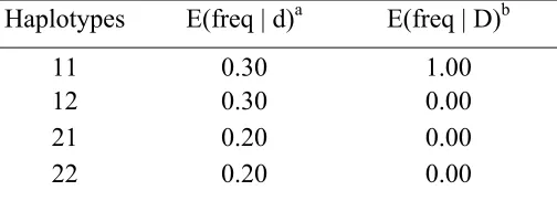
For single-marker tests, power simulations assumed that the marker and disease alleles were in perfect association. Therefore, the marker locus is in fact equivalent to the disease locus. For multiple-marker haplotype tests, two markers were simulated having four possible haplotypes (11), (12), (21), (22) with frequencies 0.3, 0.3, 0.2, 0.2, respectively. Table 2.1 shows the association configurations between these haplotypes and the disease alleles used in SIMLA.

2.4 Results

2.4.1 Type I errors and power

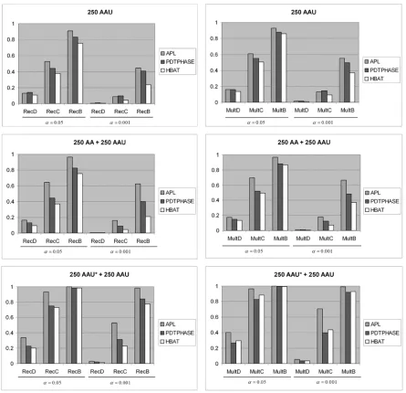
We next compared the power of the modified APL test and other family based tests of association. PDT [Martin et al., 2000a], FBAT/HBAT [Lake et al., 2000; Horvath et al., 2004] and PDTPHASE [Dudbridge, 2003] were selected for comparison since they remain valid tests for association when linkage is present. TRANSMIT was not included in the comparison since it has an inflated type I error when linkage is present [Martin et al., 2003]. Figure 1 shows the results for single-marker analysis. Compared with figure 1 in Martin et al. [2003], APL using bootstrap variance estimator obtains more power than the APL test using the original variance estimator. For example, APL using the bootstrap estimator has estimated power 0.44 at the 0.05 significance level for the RecD model for 250AAU families and the power estimate for APL using the original variance estimator under the same model is 0.32.

We also see that, for different types of family structures, the modified APL has more power than the other two methods under all genetic models considered. APL typically has an outstanding power for the RecD and MultD models. In the combined data sets with both AAU and AA families, the PDT and FBAT do not use the families without unaffected siblings. The APL test will use information from the entire collection of families. The results in figure 1 show that these AA families add a little power to the APL test for all models while the PDT and FBAT maintain the same power.

Figure 2 shows the comparison of the power of global haplotype analysis between APL, HBAT, and PDTPHASE. The pattern is similar to the single-marker results. APL continues to have more power than HBAT and PDTPHASE in most of the examples tested, and in some cases can have considerably more power.

2.4.2 Rare alleles and haplotypes

Table 2.4 also shows the adjusted type I error rate after all replicates that have estimated variances of Ts less than 2.5 and 5 were eliminated. For allele frequency of 0.01, the adjusted type I error rate becomes smaller and is often conservative, relative to the inflated rate before adjustment. Table 2.4 shows the guideline using variance 2.5 may not work well in some cases. For example, for a sample that has 100 AAU families and a rare allele with frequency 0.1, the adjusted type I error rates using a cutoff of 2.5 are inflated (0.061 and 0.058) for the RecA and MultA models, respectively. The guideline of variance 5 generally avoids inflated type I error rate shown in Table 2.4. The results of simulated data sets for disease models RecA and MultA generally show the same pattern in Table 2.4. Moreover, we can also observe the same pattern in the mixed nuclear family structures of singleton and multiplex families in Table 2.4. Note that we did not show the adjusted type I error rate using variance of 5 for the mixed family structures of 50 singleton and 50 multiplex families since only a few data sets have variance greater than 5. Hence, it is not suggested that such small sample should be tested with APL for a rare allele frequency 0.01 in real data analysis. The same pattern was observed in dominant and additive models as well using the same family structures in Table 2.4 (results not shown).

with corresponding variances of Ts less than 5 are close to the 0.05 level. We also observed

the same pattern in dominant and additive models using the same family structures. The simulation results show that requiring a variance estimate > 5 serves as a good guideline of deciding whether the APL test is valid or not when rare alleles or rare haplotypes are present.

2.4.3 HWE effect

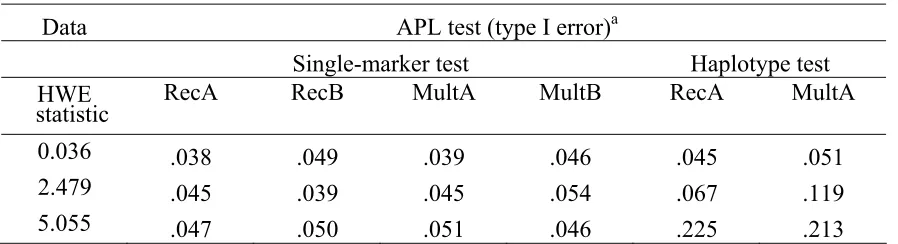
Table 2.6 shows the effect of deviations from HWE for APL single-marker analysis. It shows that even with deviations from HWE (Goodness-of-fit statistics from 0.036 to 5.055), the APL test remains valid so that the type I error under different models is close to the nominal 0.05 level. The version of APL single-marker test without the HWE assumption was also tested and found to have correct type I error rate by simulations (results not shown). The APL single-marker test with the HWE assumption is preferred since it has more power than the version without the HWE assumption, according to our simulation results (results not shown).

would be crucial for APL. Therefore, it may not be prudent to conduct haplotype analysis with the APL if there is evidence of deviation from HWE.

2.4.4 Performance

The APL program is written in C++ and available for Linux, Sun and Windows platforms. Since APL needs to perform a certain amount of bootstrap iterations, it is not as efficient as Transmit without the bootstrap option, which has the same time complexity for calculating Ts as APL. Generally APL can finish a single-marker analysis within one minute for 300 families with all parental genotypes missing. Haplotype analysis causes higher density of calculations and APL usually takes 30 minutes for a data set that has 300 families and 3 markers with all parental genotypes missing running on a Sun workstation equipped with a 1.2GHz CPU.

2.5 Discussion

model. Our simulation results showed that by using the bootstrap variance estimator, the modified APL obtains more power than the APL statistic using the robust variance estimator. We demonstrated the proper implementation of the modified APL by testing its type I error rate from different family structures and disease models.

Our simulation results showed that under different family structures, the bootstrap variance estimator correctly estimated the variance of Ts. Even when there was a mixture of different nuclear family structures, the variances were correctly estimated. In addition to the results for mixtures of multiplex families presented in Table 2.2, we also simulated a mixture of singleton and multiplex families and the type I error rate was as expected (results not shown). Hence, the bootstrap variance estimator is robust to mixed nuclear family structures.

We examined the robustness of APL for the deviations of HWE and rare alleles or rare haplotypes. HWE is assumed in the haplotype analysis to reduce the number of parameters. Though we found deviations from HWE had little impact on single-marker tests, they do affect validity of haplotype analyses. We also considered the situation when rare alleles or haplotypes are present in the data. They could affect the validity of APL statistic leading to an inflated or conservative type I error rate. When there is extensive LD between markers, rare haplotypes are more likely to exist. In this case, the global haplotype statistic may not be valid. As the TRANSMIT online manual suggests, we confirmed with simulations that variance greater or equal to 5 provides a general guideline of deciding whether to accept APL statistic or not. For global haplotype analysis, haplotypes with variance less than 5 are ignored. Another possible approach to reduce the effect of extensive LD on global haplotype analysis is to collapse rare haplotypes into one haplotype. However, the strategy of choosing which haplotypes to collapse is not trivial. The simulations presented here suggest that collapsing rare haplotypes until they exceed a variance of 5 may be a good strategy.

pedigrees and can be used as a complementary tool for APL for family-based association studies.

In conclusion, we have included several useful extensions to the APL algorithm and provided a comprehensive software package for single marker and haplotype analysis. The APL software provides a useful approach for fine-mapping complex disease genes in sibships or nuclear families that can dramatically outperform existing methods. APL can be publicly accessed at http://www.chg.duke.edu/research/apl.html.

2.6 Acknowledgements

2.7 Tables

Table 2.1 Association configurations in SIMLA for the power simulations for haplotype tests.

Haplotypes E(freq | d)a E(freq | D)b

11 0.30 1.00 12 0.30 0.00 21 0.20 0.00 22 0.20 0.00

Table 2.2 Mean, Variance and Type I error of the single-marker APL test across 5000 replicate data sets.

Data APL test

N and model of inheritance Mean Variance Type I errora N = 300 AAU:

RecA -.011 .994 .048

RecB .051 .988 .045

MultA -.013 1.018 .051

MultB -.014 1.004 .049

N = 300 AAAU:

RecA -.047 1.029 .052

RecB -.018 .991 .049

MultA -.023 .989 .047

MultB -.013 1.028 .054

N = 250 AA + 250 AAU

RecA -.028 .995 .050

RecB -.051 1.101 .051

MultA -.056 .994 .051

MultB -.035 1.010 .048

N = 200 AAAU + 100 AAU

RecA .004 .978 .046

RecB -.017 .989 .050

MultA -.014 1.025 .052

MultB -.058 .972 .047

N = 250 AAU* + 250 AAU

RecA .007 .963 .049

RecB -.021 1.009 .049

MultA -.013 1.000 .053

MultB -.023 1.047 .054

a _{Proportion of data sets with p-value ≤ 0.05.}

Table 2.3 Type I error of the multiple-marker haplotype APL global test across 5000 replicate data sets.

Data APL test

N and haplotypes Type I errora N = 300 AAU:

RecA .046

MultA .050

N = 250 AA + 250 AAU:

RecA .041

MultA .047

N = 250 AAU* + 250 AAU:

RecA .052

MultA .053

a _{Proportion of data sets with p-value ≤ 0.05.}

Table 2.4 Type I error of the single-marker APL test before and after the adjustment.

Data APL test

N and model of

inheritance E(freq)a Type I error Type I errorb Type I errorc N = 100 AAU

RecA 0.10 .065 .061 (99%d) .052 (97%)

RecAe 0.01 .069 .005 (18%) .041 (2%)

MultA 0.10 .060 .058 (99%) .047 (96%)

MultAe 0.01 .076 .006 (18%) .052 (2%)

N = 300 AAU

RecA 0.10 .053 .053 (100%) .053 (100%)

RecA 0.01 .076 .033 (77%) .020 (34%)

MultA 0.10 .051 .051 (100%) .051 (100%)

MultA 0.01 .078 .042 (76%) .023 (34%)

N = 600 AAU

RecA 0.10 .050 .050 (100%) .050 (100%)

RecA 0.01 .055 .054 (99%) .039 (33%)

MultA 0.10 .053 .053 (100%) .053 (100%)

MultA 0.01 .063 .069 (99%) .047 (88%)

N = 50 AU + 50

AAU

RecA 0.10 .066 .064 (99%) .040 (88%)

RecAe 0.01 .071 .010 (9%) N/A

MultA 0.10 .048 .048 (98%) .043 (83%)

MultAe 0.01 .078 .018 (6%) N/A

N = 150 AU + 150 AAU

RecA 0.10 .051 .051 (100%) .051 (100%)

RecAe 0.01 .061 .024 (60%) .032 (15%)

MultA 0.10 .049 .049 (100%) .049 (100%)

Table 2.4 (Continued)

Three types of family structures, 100 AAU, 300 AAU and 600 AAU, were simulated with two types of allele frequencies, 0.01 and 0.1, for the RecA and MultA models across 5000 replicate data sets. Two types of mixed family structures, 50AU (one affected child and one unaffected child) plus 50AAU and 150 AU plus 150 AAU, were also simulated. All parental genotypes are assumed to be missing.

a _{E(freq) is the expected frequency of the rare allele.}

b _{The adjusted type I error rate calculated by the proportion of data sets with p-value ≤ 0.05}

where alleles with variance < 2.5 were excluded.

c _{The adjusted type I error rate calculated by the proportion of data sets with p-value ≤ 0.05}

where alleles with variance < 5 were excluded.

d _{The percentage shows the percentage of the replicates remaining for type I error}

calculation.

e _{100,000 replicate data sets were generated for 100 families and 20000 replicate data sets}

Table 2.5 Type I error of the multiple-marker haplotype APL test before and after the adjustment.

Data APL test

Haplotypes Set1 Set2

E(freq)c E(freq)

111 0.84645 0.612

211 0.09405 0.108

121 0.04455 0.153

221 0.00855 0.027

112 0.00495 0.068

122 0.00045 0.017

212 0.00095 0.012

222 0.00005 0.003

Models Type I error

N = 300 AAU RecA:

Global test .027 .035

Global testa .044 .038

Global testb .048 .049

N = 300 AAU MultA:

Global test .021 .036

Global testa .037 .039

Global testb .047 .053

Two sets, set1 and set2, were simulated across 5000 replicate data sets with different haplotype frequencies, including rare haplotypes, for the RecA and MultA models. All parental genotypes are assumed to be missing.

a _{The adjusted type I error rate calculated by the proportion of data sets with p-value ≤ 0.05}

where haplotypes with variance < 2.5 were excluded.

b _{The adjusted type I error rate calculated by the proportion of data sets with p-value ≤ 0.05}

where haplotypes with variance < 5 were excluded.

Table 2.6 Type I error of APL tests with HWE deviations.

Data APL test (type I error)a

Single-marker test Haplotype test HWE

statistic RecA RecB MultA MultB RecA MultA

0.036 _{.038 .049 .039 .046 .045 .051}

2.479 _{.045 .039 .045 .054 .067 .119}

5.055 _{.047 .050 .051 .046 .225 .213}

300 AAU families were simulated with HWE deviations for RecA, RecB, MultA and MultB models without parental genotypes.

2.8 Figures

Figure 2.1 Power comparison for single-marker analysis

Figure 2.2 Power comparison for haplotype analysis

Chapter 3

X-APL: An Improved Family-Based Test of

Association for the X Chromosome

Ren-Hua Chung, Richard W. Morris, Li Zhang, Yi-Ju Li,

Eden R. Martin

(2007) The American Journal of Human Genetics

3.1 Abstract

tests. To show its utility and discuss interpretation in real data analysis, we also applied the X-APL to candidate gene data in a Parkinson disease family sample.

3.2 Introduction

Family-based association methods are often used for localizing genes in complex diseases when family data are available; however, methodological developments have focused primarily on analysis of autosomal markers [Spielman et al., 1993; Martin et al., 1997; 2000; Abecasis et al., 2000; Rabinowitz and Laird, 2000]. Linkage analyses have identified regions on the X chromosome for several diseases, such as Parkinson disease [Scott et al., 2001; Pankratz et al., 2003], autism [Shao et al., 2002; Vincent et al., 2005] and early-onset cardiovascular disease [Hauser et al., 2003]. Although association analysis is often applied to further localize disease susceptibility genes in linkage regions, fine-mapping of such regions on the X chromosome has been slow, in part due to the lack of appropriate statistical methods for family-based association analysis on the X chromosome.

affected siblings, can have an inflated type I error rate when linkage is present between a marker and the disease locus. This is the same problem faced by the original TDT and S-TDT [Martin et al., 1997]. Because association analyses are often conducted in regions showing evidence of linkage, it is critical that family-based association tests allow for the presence of linkage under a null hypothesis of no association when multiple affected offspring are available.

Here we extend the Association in the Presence of Linkage (APL) method [Martin et al., 2003] developed for autosomal markers to the analysis of X-chromosome markers in nuclear families. Like the APL, our proposed procedure, which we refer to as X-APL, properly infers missing parental genotypes in regions of linkage by considering identity-by-descent (IBD) parameters for affected siblings. We use a bootstrap procedure to adjust for the variation in parameter estimates, which does not assume allele frequencies are given. X-APL can perform both single-locus and haplotype association tests. Recognizing the existence of sex-limited traits, we introduce into the X-APL separate tests for males and females, which allow inference about different effects in the sexes.

3.3 Methods

The X-APL statistic is a modification of the APL statistic [Martin et al., 2003]. The APL statistic is based on the difference between the observed number of copies of a specific allele in affected siblings and the expected number of copies conditional on parental genotypes under the null hypothesis that there is no association or no linkage in nuclear families. When parental genotypes are missing, APL infers missing parental genotypes using siblings’ genotypes and accounts for linkage by taking the IBD parameters into consideration, see Martin et al. [2003] for details. The APL software can analyze families with up to three affected siblings and arbitrary numbers of unaffected siblings [Chung et al., 2006].

3.3.1 X-APL statistic

= (m,f) if one affected sibling is male and the other is female = (f,f) if both affected siblings are female

Under the null hypothesis, the expected value of Ij can be estimated conditional on the parental genotypes and sexes of the affected siblings:

⎪ ⎩ ⎪ ⎨ ⎧ = + = + = = ) , ( if 2 ) , ( if ) , ( if ) , | ( E f f sex N N f m sex N N m m sex N sex I mj fj mj fj fj pj j G

where Nfj , the number of allele 1 in the female parent, takes values 0, 1 or 2 and Nmj, the number of allele 1 in the male parent, takes values 0 or 1 in the jth family. The expected value of Ij for a singleton family has a simpler form. E(Ij| Gpj, sex = m) is (1/2)×Nfj and E(Ij |

Gpj, sex = f) is (1/2)×Nfj+Nmj. We define the statistic Tj to be Tj = Ij – E(Ij | Gpj, sex) in the jth family. In complete pedigrees, Nfj and Nmj can be counted directly from the parental data and the transmissions from male parent to affected siblings cancel in Tj; therefore, male parents provide no information for the X-APL statistic in complete pedigrees.

disease locus when inferring the missing parental genotypes. The IBD for the alleles transmitted from the male parent is fully determined by the sexes of the affected sibling pair. That is, when we consider IBD sharing for alleles transmitted from the male parent, the affected siblings share 0 allele IBD when sex = (m,m) or (m,f) and 1 allele IBD when sex = (f,f). Thus, only IBD status for alleles transmitted from the female parent needs to be estimated. The affected siblings share either 0 or 1 allele IBD from the female parent.

When there is no association and tight linkage, the probability Pr(Gp | G, A, sex) is similar to Martin et al. [2003] equation (2) and can be written as:

) , | Pr( ) , , | Pr( ) , , | Pr( 1 0 sex A sex k IBD z sex

A G k k p

p p G G G G G ∑ =

= μ = ₍₁₎

where μ_Gp is the unconditional probability of parental mating type Gp and zk is the probability that the affected siblings share k alleles IBD from the female parent. Since disease penetrances are expected to be low for any particular locus for complex diseases, transmissions to the unaffected siblings are assumed to be independent of disease status. Then IBD parameters for an unaffected sibling pair, or a pair with one affected and one unaffected sibling, can be approximated by (z0, z1) = (1/2, 1/2). Therefore, when there are unaffected siblings in a family, the probabilities Pr(G| Gp,IBD=k,sex) are multiplied by the Mendelian transmission probabilities for the unaffected siblings for given parental genotypes.

The EM algorithm is used to estimate the parameters p G

Martin et al. [2003] For singleton families, the probability Pr(G| Gp, IBD = k, sex) reduces to Pr(G | Gp, sex), which depends only on Mendelian transmission probabilities. When parental genotypes are missing, the expectation of Ij is taken over missing parental genotypes as well as transmissions from (female) parents, as follows:

= − ∑ ∈Ω

G G

G

i pi j j pi

j

j I A sex E I sex

T Pr( | , , ) ( | , ) (2) where Ω is a set of all possible parental mating types. Partial parental genotypes can be used

to improve estimation of the parental mating-type parameters, using the same methods discussed in Martin et al. [2003]. Let Ts be the sum of Tj over families, then under the null hypothesis that there is no association or no linkage, the expected value of the statistic Ts is 0. The X-APL test is based on this summary statistic Ts.

3.3.2 Variance estimation

variance Var Tˆ ( )_s can be obtained from the BTs’s. When B is large, the sample variance will be asymptotically close to the variance of Ts.

Finally, the X-APL statistic takes the following form:

) ( ˆ

s s

T ar V

T

(3)

Under the null hypothesis of no linkage or no association, this statistic is asymptotically normal, with a mean of 0 and a variance of 1.

3.3.3 Separate tests for males and females

showed that type I errors for the X-APL statistic for the sex with no disease-locus effect can be inflated when all data are used to estimate the parameters. A solution is to divide the data into two sets: one set that has only male affected siblings and another set that has only female affected siblings. The two sets may have overlapping families if some families have both affected male and female siblings. All unaffected individuals are retained in both sets. Then X-APL tests can be applied separately on the two sets using parameters estimated in their respective sets. We refer to the test using only male affected sibs and the test using only female affected sibs as X-APL male and female test, respectively. Since both male and female tests may be performed simultaneously, multiple testing should be considered when we interpret the p-values from the two tests. An adjustment for the p-values may be required such as Bonferroni correction in order to interpret the p-values properly.

3.3.4 Extension to multiple-marker haplotype analysis

disease locus, is calculated using the method in Chung et al. [2006] to measure the overall haplotype effect:

G₌T_s'_Σ−1T_{s (4)}

where the vector Ts contains the X-APL statistics for each possible haplotype, Σ is the variance-covariance matrix of Ts. If h is the number of haplotypes tested, then the statistic G

is asymptotically distributed as chi-square with h-1 degrees of freedom.

A global test for all haplotypes can be more informative than individual haplotype tests since it can capture multiple haplotype effects [Horvath et al., 2004]. The global test also can have more power than individual haplotype tests since it does not have the multiple-testing issue faced when analyzing haplotypes individually [Morris et al., 1997]. Moreover, in the X-APL test, IBD and parental mating-type parameters are estimated under the global null hypothesis that none of the haplotypes are in LD with a disease allele. It is not straightforward to estimate those parameters under a haplotype-specific null hypothesis. For these reasons, we base inference solely on the global test for haplotype analysis.

3.3.5 Hardy-Weinberg equilibrium assumption