Numerical Modeling and Experimental Verification on Sensitivity Properties of MHD Sensor

2018 International Conference on Physics, Computing and Mathematical Modeling (PCMM 2018) ISBN: 978-1-60595-549-0

Numerical Modeling and Experimental Verification on Sensitivity

Properties of MHD Sensor

Hai-jia ZHOU

, De-tian LI and Guang-feng CHEN

Science and Technology on Vacuum Technology and Physics laboratory, Lanzhou Institute of Physics, Lanzhou, 730000, China

*Corresponding author

Keyword: Magnetohydrodynamic effect, Laminar fluid, Segregated step, Magnitude-frequency characteristics, Amplitude non-linearity.

Abstract. For the insight of MHD sensor’s transferring function, the time-varying laminar flow model of magnetohydrodynamic effect was established. In the physical model the inlet and outlet, which directly drive the flows of annulus, were substituted for external walls that drive them by viscous forces. Physical model was decomposed by finite element method and iteratively solved by the scheme of segregated steps. The prototype MHD sensor was designed, fabricated, and calibrated by rotational table. Sensitivity factors of magnitude-frequency characteristics between 5 and 500Hz

from the model and the prototype were 44V/(rad/s) and 48V/(rad/s) respectively. The amplitude non-linearities of 0.02-0.10rad/s, derived from the model and the prototype, were about 2% and 5% each. The results show that sensitivity properties derived from the model are consistent with ones from the prototype sensor, which will provide a reference for improving the performance of MHD sensor.

Introduction

Magnetohydrodynamic (MHD) effect is a phenomenon that magnetic fields induce Lorentz force in the moving conductive fluid while creating electric currents and changing the original magnetic fields [1]. Based on MHD effect, MHD angular rate sensors were invented to measure angular signals in the surroundings [2,3]. The features of MHD angular rate sensor are low noise and high bandwidth without any moving mechanical parts, so they can be used in many areas, such as remotely-sensed imaging, laser communication, seismic monitoring [4-6].

The research of MHD effect stemmed from Hannes Alfvén, who was awarded Nobel Prize in 1970s[1]. Because diffusive term and coupling terms of flow field, electric fields, and magnetic field in the MHD effect, the equation sets were hard to solve. Baylis and Hunt studied the steady MHD flow in a rectangular duct, which was driven by electric fields[7]. Khal’zov and Smolyakov[8] calculated the two-dimensional MHD flows of incompressible conductive fluid in the circular duct using the iteration Gauss–Seidel method, which was used to calculate the steady-state flows. Xu et al.[9,10] analyzed the three-dimensional unsteady motion of conducting fluid in the circular container by finite volume method. Chowdhury et al. discussed the steady electric potential distributions on channel walls and inside the flow of MHD fluid using analytical and experimental method [11]. Schwarz and Fröhlich presented numerical simulations of the ascent of bubble in the liquid metal with and without an external magnetic field [12]. Bujurke analyzed the effect of surface roughness on the MHD film between two rectangular plates[13]. There are a large number of papers about numerical analysis of liquid metal MHD effect, especially the steady-state analysis. However, the sensitivity of the MHD sensor based on the time-varying numerical analysis of MHD effect is rarely reported.

Physical Model, Numerical Analysis and Testing Method Control Equations and Boundary Conditions

Assuming the density of conductive fluid  remains constant in the process, the conservation of momentum can be expressed as [14]:

△ p

t











u

u

u

u

J

B

g

where u is velocity of conductive fluid, p is pressure, J is current density, B is magnetic flux density.

According to conservation of mass, the velocity vector u needs satisfy:

0

 u  ₍₂₎

Assuming current density vector of the fluid satisfies the ohm’s law[8]:

  

 _   _

J E u B

(3) where E = - V is electric field intensity, V is electric potential among the fluid.

The current density in the fluid satisfies the conservation of current:

0

  J 

(4) Eq.1, eq. 2, eq.3 and eq.4 constitute the equation set which controls the MHD behavior of conductive fluid:                    _{  }   _{    }       △ 0 0 p t u

u u u J B g

u

J E u B

J

(5) Because conductive liquid of MHD sensor is encased into an annulus and axially symmetry, just a quarter of cylindrical conductive fluid is studied, shown in Figure 1. The sets of boundaries are

expressed as     1 2_{, where} 1 _{represents the radial boundaries,} 2 _{represents the}

axial boundaries. Then, the boundary conditions can be set as:

       _{ }      0 0 w all u n

u n U

J n

where Uwall is velocity vector of exterior wall.

When the boundaries rotate, the magnetic field inside the sensor rotates. Due to the inertia conductive fluid tends to remain stationary and cuts through the moving magnetic lines of flux. Because the moving magnetic field in the analysis is difficult to deal with, it is assumed that the annulus of conductive fluid and magnetic field are stationary while conductive fluid is driven. The driving angular velocity U core is exerted perpendicular to the surfaces of the inlet and outlet

shown in Figure 2. Then the boundary sets become the new sets,       _{1 2 3}, where

outlet) in the fluid. For the new system, MHD equation sets remain steady while boundary conditions alter into:

z-axis z-axis R2 R2 R1 R1

Uwall=

A0*r*sin(2πft)

Uwall=

A0*r*sin(2πft)

z-axis z-axis

Ucore= A0*r*sin(2πft)

Ucore=

A0*r*sin(2πft) inlet inlet outlet outlet Ucore= A0*r*sin(2πft)

Ucore=

A0*r*sin(2πft)

Uwall=0 Uwall=0

Figure 1. The original boundary conditions of MHD sensor.

Figure 2. The boundary conditions of the approximate MHD model.        _                1 2 3 3 1 2 , , 0 0 0 core u

u n U

u n

J n

(6)

Discretization and Solution

Considering that the discrete spaces of stokes problems in fluid dynamic are also fit for MHD

problems of the fluid, we adopt Lagrange polynomials, P P1 1, to discretize the space [15].

The control equation sets are decomposed using the scheme of segregated steps. Assuming the

step size of time is t , the equation sets of time t n1 can be derived from ones of time t n:

1 1 1 1 0 1 △ ( ) 0 n n

n n n n

n n n n

n t             _{     }   _{    }  _{ }       u u

u u u J B

J E u - u B

J

(7)

1

1 1 1

1

1 1 1 1

0

△

0

( )

n n

n n n n

n

n n n n

t                 _{     }   _{  }   _{    }     u u

u u u J B

u

J E u - u B

(8)

where the superscripts of physical quantities n and n+1 mark the ones of times t n and t n1, respectively.

Figure 3. The grid model of conductive fluid annulus.

Testing Method

The sensitive structure of MHD angular rate sensor is composed of magnetic loops (such as permanent magnets, magnetic yoke assemblies), electrodes and transformer, shown in Figure 4.

Figure 4. The profile of sensitive structure in MHD sensor.

The mass of the prototype MHD sensor is approximately 1Kg, and the dimension is about Φ50mm*70mm. The word length of the analog-digital converter is 16bit, and the sampling frequency is 2000Hz. The pictures of the prototype sensor and rotational table are shown in Figure 5.

Figure 5. The pictures of the prototype MHD sensor (left) and rotational table (right).

The magnitude-frequency characteristics and amplitude non-linearity of MHD sensor are calibrated using rotational table. Testing frequencies of magnitude-frequency characteristics are between 5Hz and 500Hz, and the magnitudes of input angular displacement are approximately 5-40′′. Testing frequency of amplitude non-linearity is 8Hz, and the magnitudes are about 0.02-0.12rad/s. Test results of magnitude-frequency characteristics and amplitude non-linearity are processed by Matlab.

Results and Discussion

Physical Images of Time-varying MHD Numerical Model

When the time-varying numerical model above are fed by a series of sinusoidal signals, the velocity

Permanent Magnet

Electrodes Magnetic Yoke

Assemblies Transformer

Conducting Metallic Fluid

MagneticLoops

fields and voltage fields across the conductive fluidic annulus are altering as time goes. The images of time-dependent velocity fields and voltage fields in the half cycle are shown in Figure 6 when the magnitudes of input signals are 0.01rad/s.

Figure 6. The images of velocity fields (top) and electrical potentials (bottom) in the half cycle.

The tops of Figure 6 indicate that the magnitudes of velocities in the sections perpendicular to the flowing direction are heterogeneous. The contours of velocities are similar to the sections of the walls, which is the unique phenomenon of MHD effect[14-16]. The magnitudes of velocities in the core on the time t=T/4 are nearly 1.6×10-4m/s, while the values fall down as the times deviate from the moment t=T/4 in the half cycle.

The bottoms of Figure 6 show that electrical potentials are almost distributed along the z axis in every moment. As time goes from 0 to T/4, electrical potential differences between the top and the bottom wall reach the highest about 1×10-6V on T/4, while the values drop as time continues in the half cycle.

The Analysis of Magnitude-frequency Characteristics

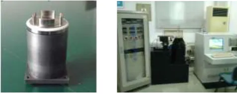
For the input sinusoidal signals of some frequencies between 0.01Hz and 10000Hz, every sets of voltage signals outputted from MHD numerical model are handled by four-parameter least square fit of sinusoid, which are partially shown in Figure 7. The expression of this least square fit is:

( ) (1)*cos(2* * (2)* ) (3)*sin(2* * (2)* ) (4)

f X a pi a X a pi a X a ₍₉₎

where a(1), a(2), a(3), a(4) are four unknown parameters, f(X) is the unknown sinusoidal objective function.

The residues of the least square fit can be expressed as:

2

[ ( i) i]

i

f X Y



(10)

where Yi is output voltages at the time Xi, f X( i) _{is objective function at Xi.}

Figure 8. Magnitudes of the output voltages in the frequency domain.

The diagram shows that the output voltages are very close to the sinusoidal objective functions under 0.1Hz and 1000Hz. The residues under 0.1Hz and 1000Hz are 5.0×10-14V2 and 6.8×10-14V2 respectively. The results of the frequencies between 0.01Hz and 10000Hz demonstrate that the voltages fit well to the sinusoid.

Using the magnitudes of the resulting sinusoidal objective functions under different frequencies of 0.01-10000Hz, frequency characteristics of the output voltages are analyzed and the result is shown in Figure 8. The result shows that the magnitudes of output voltages between 1 and 10000Hz almost remain consistent and are about 1×10-6V, while the values of 0.1Hz and 0.01Hz are 9.7×10-7V and 9.5×10-7V respectively. The differences may result from the mesh of the conductive fluid, which should be refined further.

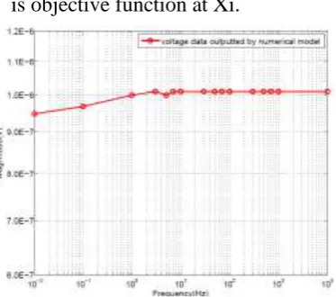
Figure 9. Frequency characteristics of the transformer in MHD sensor.

Frequency characteristics of the transformer in MHD sensor, which are the in-situ magnification part for the output voltages, are also analyzed. Some key parameters (such as primary inductance and secondary inductance) of transformer under some frequencies from 10Hz to 1000Hz are measured and analyzed. Then the curve-fitting to the magnification of the transformer under the frequencies, which is shown in Figure 9, is done. The figure shows that the magnifications of the transformer from 10Hz to 1000Hz are almost stable, the maximum and minimum are about 9.7×103 and 9.1×103, when the curve drop as the frequency increases or decreases outside the frequency band.

The sensitivities derived from MHD model and the prototype sensor are compared, shown in Figure 10. The sensitivity factors of MHD model, S , can be expressed as:

m* t* e

a

U M M

S





(11)

where Um _{is the magnitude of voltage outputted by numerical model,} Mt _{is the magnification}

of the transformer derived above, Me _{is the magnification of the circuit (here is set to 50),} a _is

angular rate inputted into numerical model.

Figure 10 shows that experimental curve between 5Hz to 500Hz is almost overlapped by the one derived from MHD model. The mean value of the prototype sensor’s and MHD model’s sensitivity factors is 48V/(rad/s) and 44V/(rad/s) respectively. There are some tiny fluctuations of the prototype’s sensitivities around the numerical model’s values in the frequencies of larger than 100Hz. I suppose that they may be originated from the bubbles in the sensor.

The Analysis of Amplitude Non-linearity

magnitudes of 0.01rad/s and 0.10 rad/s are about 1×10-6V and 1×10-5V respectively.

Figure 10. Frequency characteristics of MHD model’s and the prototype sensor’s sensitivity factors.

Figure 11. The changing voltages as the input angular rates.

Figure 12. Comparison between linear curves of output voltages.

The difference between linear curves of the output voltages derived from MHD model and the one derived from the prototype sensor is compared in Figure 12. The lines of the output voltages representing the numerical model and the prototype almost overlap. The slopes of the lines, named after standard sensitivity factor, are all 45V/(rad/s) for numerical model and the prototype. The intercepts of two lines for the model and the prototype are 9.3×10-3V and 2.5×10-2V each.

Figure 13. Change rates of sensitivity factors derived from the model and the prototype sensor.

the prototype sensor are discussed, which is shown in Figure 13. It shows that the lines representing two sensitivities are approaching. The slope derived from the model are -5V/(rad/s)2. The intercept of the line is 46V/(rad/s). The expression of the MHD model’s sensitivity factors can be conveyed:

46 5* 

  

i i

S

(12) So the input limits is 0.22rad/s and substituted into eq.12, and the amplitude non-linearity of

MHD model can be computed as:  5*0.22 / 46 100% 2%.

According to the method computed above, the prototype sensor’s sensitivity factors can be expressed as:

46 10* 

  

i i

S

(13)

The amplitude non-linearity of the prototype can be computed as:  10*0.22 / 46 100% 5%.

Conclusion

Based on time-varying MHD equations, the magnitude-frequency characteristics and amplitude non-linearities of the sensitivity are analyzed by numerical analysis and experimental verification. The frequency characteristics and amplitude non-linearities of physical model are almost the same with the results that are derived from experiment. The mean values of the MHD model’s and the prototype MHD sensor’s sensitivity factors are 44V/(rad/s) and 48V/(rad/s) respectively. The minor differences of the frequency higher than 100Hz may be stemmed from neglect of some elements in the MHD model, such as the bubbles in the conductive fluid. The linear curves of output voltages of numerical model and the prototype sensor almost overlaps, and amplitude non-linearities of the model and the prototype are 2% and 5% respectively. The verified physical model will provide a reference for optimizing the structure and improving the performance of MHD sensor.

References

[1]Magnetohydrodynamics,http://en.wikipedia.org/wiki/Magnetohydrodynamics.

[2]D.R. Laughlin. MHD sensor for measuring microradian angular rate and displacement. U.S. Patent 6173611 (2001).

[3]D. R. Laughlin. Angular motion sensor. U.S. Patent 4718276 (1988).

[4]T. Iwata, T. Kawahara, N. Muranaka, D.Laughlin. High-bandwidth attitude determination using jitter measurements and optimal filtering. AIAA Guidance, Navigation, and Control Conference (2009):1-21.

[5]J. Kaufmann, F. Hakimi, D. Boroson. Using a low-noise interferometric fiber optic gyro in a pointing, acquisition and tracking system. Proc. of SPIE 8610 (2013): 1-14.

[6]B. Pierson, W. A. Vandermeer, D. Laughlin. Rotation-Enabled 7-Degree of Freedom Seismometer for Geothermal Resource Development. Phase 1 Final Report. Technical Report (2013):1-121.

[7]J.A. Baylis, J.C.R. Hunt. MHD flow in an annular channel：theory and experiment. J. Fluid Mech 48 (1971): 423-428.

[8]I.V. Khal’zov, A.I. Smolyakov. On the Calculation of Steady-State Magnetohydrodynamic Flows of Liquid Metals in Circular Ducts of a Rectangular Cross Section. Technical Physics 51(2006):26-33.

[9]M.J. Xu, X.F. Li, T.F. Wu, C. Chen, Y. Ji. Error analysis of theoretical model of angular velocity sensor based on magnetohydrodynamics at low frequency. Sensors and Actuators A 226(2015): 116-125.

[11]V. Chowdhury, L. Bühler, C. Mistrangelo. Influence of surface oxidation on electric potential measurements in MHD liquid metal flows. Fusion Engineering and Design, 2014, 89:1299-1303.

[12]S. Schwarz, J. Fröhlich. Numerical study of single bubble motion in liquid metal exposed to a longitudinal magnetic field. International Journal of Multiphase Flow 62 (2014):134-151.

[13]N.M. Bujurke, N.B. Naduvinamani, D.P. Basti. Effect of surface roughness on magnetohydrodynamic squeeze film characteristics between finite rectangular plates. Tribology International 44(2011):916-921.

[14]Q.F. Wu, H. Li. Magnetohydrodynamic. National Defense Science and Technology University Press, Changsha, China, 2007.

[15]S. Sahu, R.P. Bhattachryay, E. Rajendrakumar. COMSOL as a tool for studying MagnetoHydroDynamic effects in liquid metal flow under transverse magnetic field. Comsol conference (2013).