1
Abstract—In this paper, we focus on developing a novel method to extract sea ice cover (i.e., discrimination/classification of sea ice and open water) using Sentinel-1 (S1) cross-polarization (vertical-horizontal, VH or horizontal-vertical, HV) data in extra wide (EW) swath mode based on the machine learning algorithm support vector machine (SVM). The classification basis includes the S1 radar backscatter coefficients and texture features that are calculated from S1 data using the gray level co-occurrence matrix (GLCM). Different from previous methods where appropriate samples are manually selected to train the SVM to classify sea ice and open water, we proposed a method of unsupervised generation of the training samples based on two GLCM texture features, i.e. entropy and homogeneity, that have contrasting characteristics on sea ice and open water. We eliminate the most uncertainty of selecting training samples in machine learning and achieve automatic classification of sea ice and open water by using S1 EW data. The comparison shows good agreement between the SAR-derived sea ice cover using the proposed method and a visual inspection, of which the accuracy reaches approximately 90% - 95% based on a few cases. Besides this, compared with the analyzed sea ice cover data Ice Mapping System (IMS) based on 728 S1 EW images, the accuracy of extracted sea ice cover by using S1 data is more than 80%.
Index Terms—Cross polarization, Machine learning, SAR, Sea ice cover
I. INTRODUCTION
ATELLITE remote sensing is among the primary tools used to monitor polar regions where severe weather conditions present great obstacles to field research. Sea ice, as one of the most important indicators of climate change in polar regions, has major impacts on the atmosphere, oceans, and terrestrial-marine ecosystem. Thus, numerous attempts have been made to monitor sea ice in polar regions.
The spaceborne radiometer (passive sensor) and scatterometer (active sensor) are two major techniques used for
The manuscript is being under second-round revision. This study is partially supported by the National Key Research and Development Project (2018YFC1407100). (Corresponding author: Xiao-Ming Li.)
X.-M. Li, Yan Sun and Qiang Zhang are with the Key Laboratory of Digital Earth Science, Aerospace Information Research Institute, Chinese Academy of
monitoring sea ice in polar regions. Observations have been widely explored to derive sea ice extent, concentration, and motion for operational service [1] – [4]. In particular, the spaceborne microwave radiometer yields the longest time-series of sea ice cover in the polar regions since 1979, showing that the average Arctic Sea ice extent is declining at a rate of 0.53 106 km2 . decade-1 [5].
Sea ice cover is a fundamental factor indicating Arctic changes. Along with the accelerating decline of sea ice and reduced ice thickness in the Arctic, sea ice cover presents more significant spatial and temporal variations in the marginal ice zone (MIZ), indicating that the satellite observations of ice cover at a higher spatial resolution than operational radiometer and scatterometer products is essential. Due to the significant advantages of high spatial resolution, polarimetric capability, and flexible imaging modes, spaceborne synthetic aperture radar (SAR) is a better solution for sea ice monitoring from a more detailed perspective. The radiometer and scatterometer can yield sea ice concentration observations across large areas with spatial resolutions of 6.25 km - 12.5 km (e.g., [6]), while spaceborne SAR can provide sea ice cover information with spatial resolutions at the scale of 1 km and up to dozens of meters. Spaceborne SARs, including Seasat, ERS-1/2, ENVISAT/ASAR, RADARSAT-1/2, TerraSAR-X/TanDEM-X and Sentinel-1, have shown good capabilities for monitoring sea ice information [7], [8], e.g., ice cover/extent [8], [9], ice classification (including ice floes, leads, polynyas) [10] – [14], ice motion/drift [15], [16], icebergs [17] – [19], and ice-wave interactions [20]. Although the methods of mapping sea ice cover or discriminating sea ice and open water from spaceborne SAR data have been proposed for a long time, such information has not been routinely used for Arctic Sea ice monitoring.
Focusing on sea open water (hereafter shortened to ice-water) classification from spaceborne SAR data, the Support Vector Machine (SVM) is a popular two-class classification machine learning algorithm. SVM-based ice-water classification methods, including pixel-based and region-based methods, have been developed for various spaceborne SAR data [8], [9], [11], [21], [22]. As the SVM is a supervised machine learning method, the most challenging task is to obtain
Sciences, Beijing, 100094, China (e-mail: [email protected]; [email protected]).
Sun is also with the University of Chinese Academy of Science, Beijing, 100049, China, Li is also with the Regional Oceanography and Numerical Modeling, Qingdao National Laboratory for Marine Science and Technology, Qingdao, China and Zhang is also with the Guilin University of Technology, Guilin, China.
Xiao-Ming Li,
Member, IEEE,
Yan Sun and Qiang ZhangExtraction of sea ice cover by Sentinel-1 SAR
based on SVM with unsupervised generation of
training data
S
well-labeled training samples, which can highlight the differences in sea ice and open water in SAR images. The training samples should be informative [23], including different sea ice types of multiyear ice, level and deformed first-year ice, new ice and many others, and different open water types, such as calm and rough sea surfaces. The acquisition of training samples, which are usually selected manually by experts, is tedious and time consuming. On the other hand, when a certain developed machine learning algorithm is adapted to other SAR data for classification of sea ice, procedures of training samples selection and re-train of the algorithm have to be repeated. Therefore, a more intelligent method of training sample generation is highly needed to develop a robust machine learning method of classifying sea ice by spaceborne SAR images.
For the ice-water classification by spaceborne SAR data, naturally, the radar backscatter intensity could be the determination basis, as the backscatter of sea ice is generally higher than that of open water, which is particularly evident in the cross-polarization channel as it is sensitive to the volume scattering while sea surface generally presents surface scattering. On the other hand, the radar backscatter of co-polarization (vertical-vertical, VV or horizontal-horizontal, HH) changes rapidly along with variation in incidence angles [8], [21], [24]. However, the radar backscatter of the sea surface in cross-polarization is slightly dependent on incidence angles and sea surface wind speed [25]; Thus, SAR cross-polarization data are proven to be more effective for ice-water classification than co-polarization SAR data [7]. Therefore, some recently proposed ice-water classification methods are based on the dual-polarization (HH and HV) SAR data of RADARSAT-2 [8], [9], [11], Sentinel-1 [21], [26], [27] and Gaofen-3 [22].
Although the SAR radar backscatter of sea ice and open water may have similar characteristics under some conditions, their texture features calculated based on the intensity can have differences. Therefore, instead of using only radar backscatter intensity, texture features are additionally used for classifying sea ice and open water. Various studies on texture analyses of SAR images have demonstrated that the gray-level co-occurrence matrix GLCM texture features can effectively reflect specific backscatter (or intensity) patterns that are different between ice types and open water [28] – [30]. Previous studies [10], [12], [28] suggest that the texture features of energy, contrast, correlation, homogeneity, entropy, and moment are informative for ice classification.
In this study, an SVM-based classification algorithm is proposed for ice-water classification in the Arctic. By introducing the GLCM texture features into the step of extracting and classifying training samples, the unsupervised generated training samples take the place of costly, manually labeled training samples. Moreover, different from previous relevant studies, the training samples generated by the proposed method are variable from one case to another one, to better be suitable for significant variations of sea ice conditions in the marginal ice zone (MIZ) of the Arctic. This idea has been preliminarily tested in a few Chinese C-band SAR Gaofen-3 cross-polarization images [22]. In this study, the algorithm is
further improved and applied to the S1 extra-wide (EW) swath data in HV polarization, and extensive validation is conducted for the EW data acquired in the Arctic.
II. DATASETS
A. Sentinel-1 Extra-Wide Swath Data
For the algorithm development and validation, 728 scenes of S1A and S1B EW data in HV polarization acquired in the Arctic during the melting season from July 1 to September 30, 2018, were used. Prior to using these data to derive sea ice cover information, all these HV-polarized EW data are denoised using the method proposed in [31].
The EW data have dimensions of approximately 10000pixels in both azimuth and range directions. Although we have achieved parallel computation of GLCM to derive texture features (which is described in detail in Section III), the EW HV-polarized data are resampled by spatially averaging to half the size of its original dimension, leading to the pixel size being changed from 40 by 40 m to 80 by 80 m, which significantly improves the efficiency of GLCM textures computation.
B. IMS Data
The Multi-sensor Snow and Ice Mapping System (IMS, https://nsidc.org/data/G02156/versions/1) sea ice extent data produced by the National Snow and Ice Data Center (NSIDC) are used for comparison with the S1-derived sea ice cover results. The sea ice information derived from the passive microwave (radiometer), active microwave (SAR) and optical (multiple spectra) remote sensing sensors, as well as in situ data, are used to produce the IMS sea ice product. These data are considered valid at 0:00 UTC each day. The analysts compile the sea ice cover map based on the collected satellite imagery and other data acquired over different times within a day [32]. In this study, the IMS data at a spatial resolution of 1 km by 1 km are used for comparison.
C. GSHHS Data
The Global Self-consistent Hierarchical High-resolution
Geography Database (GSHHG,
https://www.ngdc.noaa.gov/mg
g/shorelines/gshhs.html) is used for masking land presented in S1 EW images. The full resolution product in a 1 1 arc-minute grid of version 2.3.7 was released in 2017.
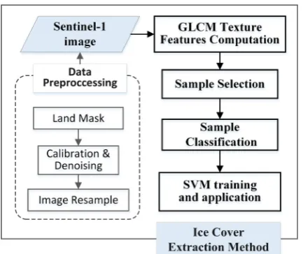
III. METHODOLOGY
Fig. 1. Flowchart of the proposed method for deriving sea ice cover from S1 EW data in HV polarization.
A. Calculation of texture feature using GLCM
GLCM, which was first proposed by Haralick et al. [33], is a widely applied method for texture feature extraction. The GLCM represents the distance and angular spatial relationship over an image subregion of a specific window. The GLCM calculates how often a pixel with gray level (also called gray tone) value 𝑖 occurs either horizontally, vertically, or diagonally to adjacent pixels with value 𝑗.
Four key parameters that need to be set in the GLCM calculation, i.e., number of gray levels b, window size (dimension) w, direction θ, and distance d. Based on the GLCM in one sliding window, one value per pixel position of each texture feature (introduced below) can be acquired. Then, the step size s of the sliding window that determines the spacing resolution of the texture features can be selectively set according to the research demands.
In this study, the number of gray levels 64, the orientation of 0°, 45°, 90°, and 135° are chosen based on previous studies, e.g., [10], [28]. We conducted a series of experiments with the S1 EW data to test the parameters of window size varying from 16 to 64 pixels and the distance varying from 4 to 16 and verify which setting of the parameters can highlight the discrimination between sea ice and open water. Finally, we decided to set the window size to 24×24 pixels, the distance to 6 pixels. The step size was set to be 12 pixels, i.e. the pixel size of the SAR-derived sea ice cover data is 960 m (12 pixels*80 m/pixel), which is convenient for comparing the SAR-derived sea ice cover with the IMS data with a grid size of 1000 m. In principle, one can reduce the step size to obtain sea ice cover information in higher spatial resolution.
Texture features reflect the visually changing features in the image. Numbers of textures can be extracted using GLCM [28], [30], [33], while some of them are highly correlated and therefore do not need to be used repetitively in the classification. Based on other studies (e.g., [10], [12], [30]) and our previous work on X-band [11] and C-band [22] SAR data, the mean intensity and other five textures, i.e., energy (also known as angular second moment [33]), entropy, contrast, correlation,
and homogeneity, are determined to be more useful for ice-water classification. These six parameters are defined in the following:
I̅ ∑ ∑ (1)
𝑒𝑛𝑒𝑟𝑔𝑦 ∑ ∑ 𝑠 𝑖, 𝑗 (2)
𝑒𝑛𝑡𝑟𝑜𝑝𝑦 ∑ ∑ 𝑠 𝑖, 𝑗 𝑙𝑜𝑔 𝑠 𝑖, 𝑗 (3)
𝑐𝑜𝑛𝑡𝑟𝑎𝑠𝑡 ∑ ∑ 𝑖 𝑗 𝑠 𝑖, 𝑗 (4)
𝑐𝑜𝑟𝑟𝑒𝑙𝑎𝑡𝑖𝑜𝑛 ∑ ∑ , (5)
ℎ𝑜𝑚𝑜𝑔𝑒𝑛𝑒𝑖𝑡𝑦 ∑ ∑ , (6)
I̅ is the mean intensity values of pixels in a window 𝒘 with dimensions of 𝑚 columns and 𝑛 rows. 𝑖, 𝑗 is the pixel pairs of grayscale, and s i, j is the frequency value of the pixel pairs
𝑖, 𝑗 in the GLCM. 𝑢 , 𝑢 are the mean frequency values of rows and columns, respectively, and 𝜎 , 𝜎 are standard deviations, which are computed as follows:
𝑢 ∑ ∑ 𝑖 ∗ 𝑠 𝑖, 𝑗 (7)
𝑢 ∑ ∑ 𝑗 ∗ 𝑠 𝑖, 𝑗 (8)
𝜎 ∑ ∑ 𝑖 𝑢 𝑠 𝑖, 𝑗 (9)
𝜎 ∑ ∑ 𝑗 𝑢 𝑠 𝑖, 𝑗 (10)
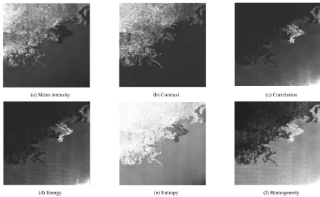
Fig. 2 shows the six texture images derived from a denoised S1 EW HV-polarized image using the method proposed in [31]. As expected, these texture features show distinguishable differences between sea ice and open water that sea ice usually presents more randomness and complexity variations in the SAR images. Therefore, it has larger values of contrast and entropy textures than those of open water. In contrast, as the open water is rather smooth with more regular and stable textures, higher values of correlation, energy, and homogeneity are presented. These opposing trends in sea ice and open water textures, particularly the most distinct ones of energy, entropy and homogeneity, yield the possibility of sample classification. In Fig. 2, there is a region close to the distinct sea ice boundary appearing extremely low backscatter values, which might be frazil or grease ice. Frazil or grease ice has different thicknesses and radar backscatter characteristics of different phases during forming [34]. This area presents high values of correlation, energy and homogeneity textures, similar to those of open water.
(a) Mean intensity (b) Contrast (c) Correlation
(d) Energy (e) Entropy (f) Homogeneity
Fig. 2. Image textures of an S1 EW image in HV polarization acquired on September 26, 2018 over the Beaufort Sea. (a) - (f) are the corresponding nomalized mean intensity value, contrast, correlation, energy, entropy, and homogeneity, respectively. Image ID: S1A_EW_GRDM_1SDH_20180926T164932_20180926T165032_023872_029AF3_4D04.SAFE
B. Extraction of Training Samples
The core idea of extracting samples is to use the watershed transformation to segment the homogeneity and entropy texture images independently based on their gradient magnitudes to polygons (i.e. the so-called “catchments”) of “pure” sea ice and open water samples. The watershed transformation is a region-based segmentation approach. Sea ice and open water presented in S1 images often are widely connected with no obvious watershed ridges existing (leading to under-segmentation), and the watershed transformation is sensitive to details and noise (leading to over-segmentation) in the image. Therefore, the marker-controlled watershed image segmentation (e.g., [35]) is applied in this study, which is accomplished based on the MATLAB tools in our study.
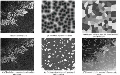
The watershed transformation is applied twice in the sample segmentation processing. The first transformation is conducted on the local gradient minima of several sub-regions to extract the edges of the Euclidean distance transform. Then, the morphological reconstruction of the gradient magnitude is conducted by using the first watershed ridges as foreground markers and the local minima as background markers. After all these, the second transformation is conducted on the marker-controlled gradient magnitude to obtain the resulted sample segmentation. Fig. 3 shows the step-by-step breakdown process of sample segmentation in a texture image of homogeneity.
Step Ⅰ: The Sobel operator is used to calculate gradient magnitude of the homogeneity texture, as shown in Fig. 3(a).
We can see that there are no obvious edges in the large areas of ice and water covered in Fig. 3(a). Therefore, in the following steps, we need background and foreground markers to obtain the catchments that are desired for extracting training samples by the watershed transformation. To evenly obtain training samples over the whole EW images, we divided the whole Fig. 3(a) into 10×10 segmented subregions (i.e. sub-images) to find the local minima of the gradient magnitude. Each subregion generates at least one minimum gradient (green dots in Fig. 3(b)), and then a binary matrix is built with values of 1 in the minima pixels and 0 in other pixels. These minimum points are used as background markers in step III.
Step Ⅱ: Based on the binary matrix (minima or not) obtained in the first step, we get the Euclidean distance transform, as shown in Fig.3(b). In the figure, the white edges are the boundaries in which the pixels have the same distances to every two adjacent minima (the green dots). The gradient gray represents the increased Euclidean distance from the minima to the edges. We accomplished this process in MATLAB by using the function called “bwdist”.
edges of these polygons are used as foreground markers in Step III.
(a) Gradient magnitude (b) Euclidean distance transform (c) Polygons achieved after the first watershed transformation
(d) Morphology reconstruction of gradient
magnitude (e) Polygons after the second watershed transformation (f)Obtained training samples in homogeneity image Fig. 3. Intermediate results of extracting samples using the marker-controlled watershed transform method for the case presented in Fig.2. The processing details are presented in the main text.
Step Ⅲ: The morphology reconstruction of the gradient magnitude is accomplished by using the minima as background markers and the edges of polygons as foreground markers. The principle is to modify the gradient magnitude image so that its only regional minima occur at the binary marker pixels. Comparing to Fig. 3(a), the gradients after the morphology reconstruction shown in Fig. 3(d) are smoothed and highlighted, while the black dots and watershed ridges replaced the darkest areas in the gradient image. This process was accomplished by using the MATLAB function imimposemin.
Step IV: The second watershed transformation is applied to the marker-controlled gradient magnitude, and the extracted polygons are shown in Fig. 3(e), i.e., the polygons filled in light gray tones. Fig. 3(f) shows the final extracted sample polygons superimposed in the homogeneity texture image, where the training samples are evenly distributed throughout the whole image. Most of these samples are pure sea ice or open water, though there are few polygons (4 ones among the extracted 100 polygons of this case) include mixture samples.
Similarly, the above described processing is also applied to the entropy texture image to extract the respective training samples.
C. Classification of Training Samples
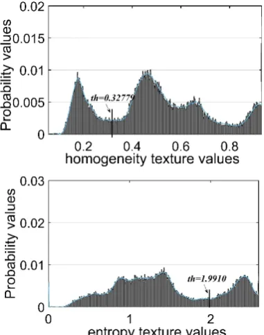
Fig. 4. Type Ⅰ: the typical bimodal histograms of homogeneity (upper) and
entropy (lower) texture features. The thresholds exist between the two peaks. Fig. 5. Type Ⅱ: the typical “large homogeneity” histograms of homogeneity (upper) and entropy (lower) texture features.
Fig. 6. Type Ⅲ: the typical “small homogeneity” histograms of homogeneity
and entropy texture features. Fig. 7. Type Ⅳ: the typical other multimodal histograms of homogeneity and entropy texture features.
Fig. 4 shows the bimodal probability distribution histograms of the two textures of entropy and homogeneity that presented in Fig. 2. By applying Otsu's method to the histogram of homogeneity texture, the threshold of 0.24164 is determined, and the same is done for the histogram of entropy texture with a threshold of 2.2812.
Although Otsu's method performs well in cases with bimodal histograms, the histograms of textures are often multimodal due to complicated sea ice and open water conditions. In our
experiments, we utilized the major thought of Otsu's method that using a histogram to find the valley value between two classes. We conclude with nearly all possible conditions into four typical cases to build the criterion of threshold computations. The four group histograms of Fig. 4 to Fig.7 are acquired from four single images that belong to the four cases respectively, in which the thresholds are obtained independently in each image.
texture of the image that is dominated by a large area of open water (the case presented later in Section IV, Fig. 11(a)). In this case, the lesser amount of sea ice has the lowest homogeneity values and the highest entropy values, whereas the open water has a large range and densely distributed texture values that present as the high peaks in Fig. 5(a) and (b). According to the contrasting characteristics of the two textures, we use the homogeneity histograms for explanation hereafter. Different to Fig. 4(a), the major peaks corresponding to open water in Fig. 5(a) exist in the last half of the histogram. Thus, instead of the valley values between the two large peaks, the threshold is selected at the front of the major peaks.
Conversely, Fig. 6 shows the two texture histograms of the image dominated by a large area of sea ice (the case presented in Fig. 12(a)). In this image, the lesser amount of water has the highest homogeneity values and the lowest entropy values, whereas the sea ice has a large range and densely distributed texture values that present as the high peaks in Fig. 7. The determined homogeneity threshold is selected following the high peaks, and the entropy threshold is selected close ahead of the high peaks.
Generally, in the homogeneity texture histogram, the stronger the sea ice radar backscattering is, the lower the texture values of the first peak (corresponding to sea ice) will be; and the more concentrated the sea ice radar backscattering is, the higher the first peak probability will be. No matter the size of the first peak, it most likely represents sea ice. As shown in Fig. 7, in the fourth type with multimodal histograms, the thresholds can be selected at the tail behind the first peak, while the thresholds of the corresponding entropy histograms can be selected at the front of the last peak.
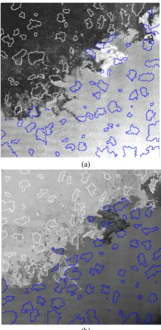
After acquiring the thresholds from the homogeneity and entropy texture histograms, the samples are classified. Taking Fig. 4 as an example, once the average homogeneity value of one sample polygon is lower than the determined threshold with a value of 0.24164 or the average entropy value is higher than the threshold of 2.2812, the sample is classified as sea ice ( white polygons in Fig. 8(a)). Otherwise, it is classified as open water (blue polygons in Fig. 8(b)). Note that we used the unnormalized texture values to compute the thresholds.
During our studies on determining thresholds to classify training samples following the steps described in Part B, it is found that the Otsu method does not perform accurately for many cases. Therefore, we tried to adjust and optimize the pre-determined thresholds (using the Otsu method) based on visual interpretation of SAR texture images and their corresponding histograms. The threshold is optimized by comparing the peaks and troughs in the histograms with the observed sea ice and open water in texture images. By processing numbers of SAR images, we can get a general rule of determining the threshold and apply to other cases.
(a)
(b)
Fig. 8. The classified sea ice samples (white polygons) and open water samples (blue ones) in the homogeneity (a) and entropy (b) texture images. Mean radar backscatter and all the texture features of these samples are used to train the SVM.
D. Application of SVM
In addition to the homogeneity and entropy textures of the selected training samples, we add other four textures of these samples to train the SVM. The LibSVM (developed in [37]) is used for the training and implementation of the SVM, where the Gaussian kernel function is applied. For the demonstration case, an image size of 9992 by 10320 pixels was first resampled to half size, with the pixel size reduced to 80 m by 80 m. The GLCM is calculated in a 24×24 pixel sliding window with a sliding step of 12 pixels. Therefore, the final SAR-derived sea ice cover data have a pixel size of 960 m.
Fig. 9(b) shows the extracted sea ice cover in this case using the processed method, where the sea ice is white and open water is cyan. We also derived the sea ice boundary by visual inspection, shown as red lines in Fig. 9(a), to evaluate the comparison result using the parameter accuracy. The correctly classified sea ice and open water pixels are recorded as True Positive (TP) and True Negative (TN), respectively [13]. Then the accuracy is defined as:
𝐴𝑐𝑐𝑢𝑟𝑎𝑐𝑦 ∙ 100% (11)
accuracy of the SAR-derived result using the proposed method is 96.30%, suggesting a good consistency with the visual inspection result. The particularly dark spot was interpreted as grease ice (refer to the main text of Fig.2), which has similar texture pattern with the calm water. Thus, the proposed method does not discriminate it from open water. And due to the uncertainty of identifying this region to be grease ice or open water, it is not confirmed as sea ice cover in the visual inspection result.
For each S1 EW image in HV-polarization, the above described steps, i.e. selecting training samples based on watershed transformation, classifying these samples based on contrast texture of homogeneity and entropy and the subsequent training and application of SVM, are conducted independently. In the following Section, more cases of extracting sea ice cover information based on the proposed method and their comparisons with other products are presented.
(a) (b) (c)
Fig. 9. (a) Visual interpretation of sea ice cover (the boundary is marked by the red line), (b) extracted sea ice cover (white) using the S1 EW image, and (c) the comparison of the SAR result with visual interpretation. The accuracy of sea ice cover in this case is 95.6%. Taking the visual interpretation as the actual ice cover, the white and blue indicate the correctly classified sea ice (TP) and open water (TN) pixels, and the pinkand green indicate the wrongly classified sea ice (FP) and open water (FN) pixels. The same colors used in the following comparisons.
IV. RESULTS AND VALIDATION
In this section, we present the comparisons of the SAR-derived sea ice cover results with visual inspection results based on a few cases, and with the IMS data based on a large amount of EW data(728 scenes)acquired over the MIZ in Arctic ocean. Further, we presented a few cases in winter season to demonstrate that the proposed method has good applicability to classify sea ice in different seasons.
A. Comparison with the visual inspection results
Fig. 10 presents four images (two cases in the summer of 2017 and another two ones are in the summer of 2018) of derived sea ice cover by S1 EW data and their comparisons with the visual interpretation results. The accuracies of the four cases are 95.6%, 96.1%, 89.2% and 97.3%, which suggests that the sea ice and open water were overall well classified based on the proposed method. The proportions of TP, TN, FP, and FN to the number of the total pixels of the four cases are listed in Table. 1. The values in Table 1 generally indicate that the fraction of mismatched open water pixels is higher than that of sea ice. The MIZ is generally defined as the transition between the open ocean and sea ice, where the mixture of sea ice and open water is complicated. The case shown in (c) and (g) have
compact edges of sea ice, therefore, the comparisons show good consistency between the detection and the visual inspection results. The case shown in (e) presents the situation of both dense pack ice and thin ice existing. While the later has low radar backscatter, close to that of open water, a large fraction of FN (the mismatch of open water pixels) is found in this case. On the other hand, even visual inspection of discriminating thin ice and open water in this case becomes difficult, which can cause bias of drawing the sea ice boundaries.
Because it is not possible to evaluate the SAR-derived sea ice cover for a large amount of data compared with visual interpretation, we choose the IMS sea ice cover data for further comparison.
TABLE I
The proportions of TP, FP, TN and FN in the full S1 image pixels of the four cases presented in Fig. 10.
Image ID TP FP TN FN
8ADD 27.9% 2.2% 67.8% 2.2%
F320 43.7% 0.50% 52.40% 3.40%
1CC3 19.8% 0.6% 69.4% 10.2%
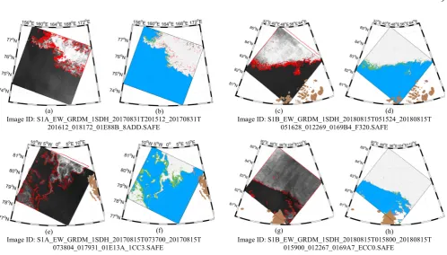
(a) (b) (c) (d) Image ID: S1A_EW_GRDM_1SDH_20170831T201512_20170831T
201612_018172_01E88B_8ADD.SAFE
Image ID: S1B_EW_GRDM_1SDH_20180815T051524_20180815T 051628_012269_0169B4_F320.SAFE
(e) (f) (g) (h)
Image ID: S1A_EW_GRDM_1SDH_20170815T073700_20170815T
073804_017931_01E13A_1CC3.SAFE Image ID: S1B_EW_GRDM_1SDH_20180815T015800_20180815T 015900_012267_0169A7_ECC0.SAFE
Fig 10. Four cases of S1 EW images (a, c, e, and g) in cross-polarization where the sea ice boundaries are interpreted by visual inspection. Their corresponding extracted sea ice cover results using the proposed algorithm are shown in (b), (d), (f), and (h), respectively. The accuracies of the four cases are 95.6%, 96.1%, 89.2% and 97.3%. The land is masked by brown in the images, which is the same for other images.
B. Comparison with the IMS data
To evaluate the overall accuracy of the proposed method, we derived sea ice cover from 728 scenes of S1 EW data, which was acquired during the summer season (July to September) of 2018 in the Arctic. For better validation of the ice-water classification results, the EW data acquired during this period with sea ice coverage of the entire image not in the range of 10% to 90% (using the IMS product as a reference) are not included in the validation dataset. The reason for data screening is that both the threshold determination with the Otsu’s method and the SVM training would simply fail if there are not two distinct classes in one single image. Besides this, we also discarded those data with a land proportion of more than 90% to reduce instability that may be caused by the inaccuracy of land mask.
The extracted sea ice cover data have a pixel size of 960 m, which is close to the resolution of the IMS sea ice data (1 km); therefore, these data are matched with the IMS data on a pixel-by-pixel basis. We first present three examples of the S1-derived sea ice cover with the IMS data, as shown in Fig. 11 to Fig. 13. The accuracies of the extracted sea ice cover in these three cases are 82.3%, 92.3% and 73.3%. These three cases highlight the advantages of sea ice detection using spaceborne SAR with a high spatial resolution to map sea ice cover in MIZ.
Fig. 11. A case of S1-derived sea ice cover and its comparison with the IMS data: (a) the denoised S1 image in HV polarization, (b) the extracted sea ice cover using the proposed method, (c) the IMS sea ice chart, and (d) the
match-up between (b) and (c). (ID:
Fig. 12. The same as Fig. 11 but for the case acquired on Aug. 22, 2018 (ID: S1B_EW_GRDM_1SDH_20180822T132251_20180822T132351_012376 _016D10_A313.SAFE)
Fig. 13. The same as Fig. 12, but for the case acquired on July 14, 2018 (ID: S1B_EW_GRDM_1SDH_20180714T030454_20180714T030554_011801 _015B6D_56DD.SAFE)
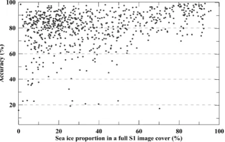
Fig. 14 shows the comparison of the extracted sea ice cover derived from the 728 EW scenes with the IMS data, along with the sea ice proportion (i.e., the proportion of sea ice cover in the full coverage of S1 image) variation, and the corresponding statistical result of the accuracy is shown in Fig. 15. Note that we used the SAR-derived results to recalculate the proportions of sea ice and used them as the x-axis values in Figs. 14 and 15. The overall accuracy of the 728 cases is 80.3%. Forty-nine cases have accuracies below 60%. Many of the cases with low accuracy have the circumstances of the radar backscatter intensities of newly formed sea ice similar to those of open water, which breaks the principle that using a threshold to accurately segment the sea ice and open water samples, therefore leading to misclassifications. The mean accuracy of all cases along with sea ice proportion is rather stable, which
varies between 77.5% and 88.1%, and the standard deviation varies from 10.4% to 15.2%.
The accuracy of S1-derived sea ice cover compared with IMS data is relatively lower than the comparisons with the visual interpretation results. This should have two reasons. On the one hand, the IMS data are produced using various satellite data, which have different spatial resolutions and may lead to smoother results in the process of data fusion, while the SAR-derived sea ice cover in this paper is pixel-based. On the other hand, multi-sensor satellite data used for generating the IMS daily products are acquired at different time, while the SAR-derived results are snapshots of the sea ice conditions at the SAR data acquisitions. The temporal variation in sea ice can also lead to some differences between the SAR observation and the IMS data.
Fig. 14. Variation in the accuracy of sea ice cover derived from the 728 S1 EW images in HV polarization acquired during July 1 to September 30, 2018 along with the sea ice proportion of the full image cover.
Fig. 15. The average accuracy values (dots) and the standard deviation (error bar) for different proportions of sea ice cover of full SAR image covers. The accuracy is rather stable, with a variation between 77.5% and 88.1%, and the standard deviation varies from 10.4% to 15.2%.
has low radar backscatter. In the homogeneity texture image shown in Fig. 16(b), the values of the sea ice are very close to those of the windy sea surface, particularly in the lower right region. The algorithm finds the thresholds in the histograms of homogeneity (Fig. 16(c)) and entropy (Fig. 16(d)), and eventually, we obtain the extracted sea ice cover, as shown in Fig. 16(e). Obviously, the sea ice in the upper-left region is misclassified as open water. In this case, the two types of samples cannot be segmented automatically by only the homogeneity and entropy textures. This is also the main reason that the 49 scenes have low accuracies in terms of sea ice detection. Moreover, the validation dataset is taken in the melting season of Arctic, therefore, the surface of sea ice is wet, which may also cause their textures similar to those of open water and the consequent misclassification, particularly when the sea surface is rather rough. Thus far, this is a weakness in the proposed algorithm. Even by manually classifying the training samples by visual interpretation, the SVM cannot achieve a good ice-water classification result in this case. In further development, better characteristics are needed to distinguish between the two types.
(a) (b)
(c) (d)
(e)
Fig. 16. An example of an S1 EW image in cross-polarization presenting thin ice and windy sea surface that is not correctly classified when using the proposed method. (a) denoised S1 EW image, (b) its homogeneity texture image, and (e) extracted sea ice cover using the training samples determined by the histograms of (c) homogeneity and (d) entropy texture features. (ID: S1B_EW_GRDM_1SDH_20180711T073722_20180711T073822_011760 _015A2A_A0C7.SAFE)
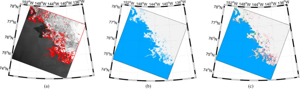
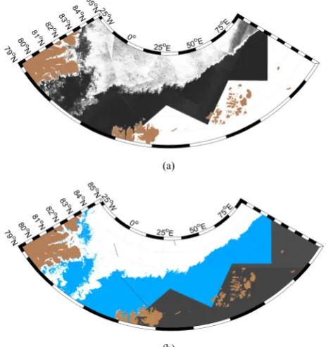
Besides, in Fig. 17, we present a relatively large panorama of the Greenland Sea, the Barents Sea and the surrounding sea areas with a longitude range of 29°W to 90°E and latitude range of 79° N to 85°N, which was assembled from 13 S1 EW images obtained on August 15, 2018 between 03:53 and 12:04 UTC. This panorama highlights the advantages of spaceborne SAR in detecting sea ice in the MIZ, and it also illustrates that the proposed algorithm performs well in classifying sea ice and open water with good accuracy.
(a)
(b)
Fig. 17. (a) The mosaic denoised S1 images and (b) the extracted sea ice cover based on 13 images acquired in the Arctic between 03:53 and 12:04 UTC on August 25, 2018. The white regions in (a) represent the S1 data with full open water cover.
C. Cases in the winter season
All the cases and statistical analyses presented above are based on the S1 HV-polarized images acquired in the melting season. This is because in the melting season, sea ice at the MIZ in the Arctic present significant spatial and temporal variations, while we would like to highlight the advantages of mapping sea ice cover by spaceborne SAR in high spatial resolution. Early studies (e.g., [38]) have shown that sea ice in different seasons can present variable radar backscatter characteristics in SAR images. Therefore, in this section, we present two cases to demonstrate the application of the proposed method to S1 data acquired in the winter season to extract sea ice cover. Note that the proposed method is not intended to apply to extract sea ice cover from S1 HV-polarized data acquired in specific seasons. In other words, we expect that the method can perform well for sea ice in different seasons.
right column of the figure. The two cases were acquired in the Kara Sea, and the Greenland Sea, respectively. The extracted sea ice cover is in good agreement with visual inspection of the original S1 images. In the Kara Sea case, the sea ice closed to the southeast coast of the archipelago presents similar radar backscatter feature with that of the surrounding open water, which was not well classified by the proposed method. The sea ice was well classified in the Greenland Sea case, which presents highly spatial variations of sea ice. This is an interesting case as well, one can observe the runoff pattern (the
bright linear feature elongating from land to open sea) of freshwater from the melting glacier to the open sea, which should contribute to the significant spatial variation of the sea ice over that region.
While the two cases indicate that the proposed method generally can discriminate sea ice and open water in the winter season, more S1 data need to be analyzed to examine the discrepancy of performance of the proposed algorithm on data acquired in different seasons.
(a)
ID: S1A_EW_GRDM_1SDH_20190104T030737_20190104T030837_025322_02CD45_23FA.SAFE (Kara Sea)
(b)
ID: S1A_EW_GRDM_1SDH_20181202T083009_20181202T083109_024844_02BC4B_D07D.SAFE (Greenland Sea)
Fig.18 Two cases to demonstrate the application of the proposed method to S1 data acquired in the winter season to extract sea ice cover.
V. SUMMARY AND CONCLUSIONS
The two SAR sensors carried by S1A and S1B have been acquiring images in wide swath (~ 400 km) HH and HV polarizations, and these sensors are dedicated to monitoring sea ice in the Arctic. The SAR data in cross-polarization are suitable for sea ice detection, mainly because these data are less sensitive to incidence angles and sea surface roughness compared with the co-polarization data. However, compared with spaceborne radiometers and scatterometers, the high spatial resolution of SAR is a unique advantage. While sea ice melting in the Arctic is accelerating, sea ice observations of fine
features in MIZ has drawn more focus for investigations of interactions among ocean surface dynamics and sea ice, as well as for shipping safety in the Arctic. Therefore, we aim to develop an effective algorithm to derive sea ice cover using S1 EW data.
selecting these samples to cover as many conditions as one can. When analyzing the texture features of hundreds of EW images acquired in the Arctic MIZ, we found that sea ice and open water generally have contrasting GLCM textures because of their different polarimetric characteristics on the cross-polarization data. Therefore, we expect to generate the ice and water training samples without supervise based on textures, specifically, homogeneity and entropy textures. Following the generation of training samples, the SVM training is conducted using all parameters, i.e., mean radar backscatter, and six textures of contrast, correlation, homogeneity, energy and entropy of these samples. Then, the trained SVM is applied to the full EW image and discriminate sea ice from open water. The key point is that we do not have a set of “fixed” training samples of sea ice and open water for a “fixed” SVM and then apply the model to all images; instead, the training samples vary along with sea ice and open water condition changes from image to image. Thus far, we had applied this method to the C-band SAR data of S1 in EW mode and the Chinese GF-3 data in stripmap mode [22]. We had also tried the proposed method using the X-band TerraSAR-X and presented the result in the TerraSAR-X/TanDEM-X science meeting 2019.
The algorithm is validated by comparing the SAR-derived sea ice cover (from 728 scenes of images) to the IMS data. The overall accuracy is 80.3%. As the daily IMS data are compiled based on various satellite observations within a day, we infer that it may not present spatial and temporal variations of sea ice due to the used data with different spatial resolutions and acquisition times. This can lead to discrepancies in sea ice cover between the SAR observations and the IMS data. Although the comparison with visual inspection were conducted in only four images, higher accuracy of approximately 90% are achieved. In addition to the validation was conducted for a dataset acquired in summer season, we present two cases of the S1 data acquired in winter season to demonstrate applicability of the proposed method. The results are also in good agreements with visual inspection, which are not surprising to us because the method is based on contrasting textures of sea ice and open water. Although melting of sea ice or snow accumulated on sea ice can change radar backscatter to some extent, it does not alter such contrasting trends.
As noted in the Section IV discussion, a weakness of this algorithm is that it can misclassify sea ice (e.g., thin ice) that has very similar radar characteristics to that of open water, especially the rough sea surface. This limitation is because their texture features are quite similar and therefore the thresholds to classify training samples cannot be accurately determined. We have not yet found a reasonable solution to this misclassification.
In the proposed algorithm, the EW data in HH polarization (acquired simultaneously with the HV polarization) is not used. We also attempted to add the HH-polarized data (as well as polarization ratio or polarization difference between HH and HV) to the SVM, but the result did not improve.
Machine learning is certainly a good means of detecting sea ice by spaceborne SAR data. The SVM based methodology is a traditional way of classifying two types of objects, e.g., sea ice
and open water. There are also other supervised algorithms available for the ice - water classification (e.g., presented in [26], [27]). However, we still face some challenges, e.g., our brains tell us what is sea ice and what is open water in the SAR images, whereas the detected results of some cases are not ideal. We are now moving to deep learning, e.g., using the good results achieved in the SVM classification as training for a deep learning network.
ACKNOWLEDGMENT
The S1 SAR data are downloaded from the Copernicus data hub (https://scihub.copernicus.eu/). We would like to thank ESA for providing the S1 data available for worldwide users. Use of the reference data of IMS data (https://www.natice.noaa.gov/ims/) and GSHHG data (https://www.soest.hawaii.edu/pwessel/gshhg/) is also acknowledged.
REFERENCE
[1] J.C. Comiso, D. J. Cavalieri, C. L. Parkinson, P. Gloersen, “Passive microwave algorithms for sea ice concentration: a comparison of two techniques” Remote Sens. Environ., vol. 60, no. 3, pp. 357-384, Jun. 1997. [2] N. P. Walker, K. C. Partington, M. L. V. Woert, T. L. T. Street, “Arctic sea ice type and concentration mapping using passive and active microwave sensors”, IEEE Trans. Geosci. Remote Sens., vol. 44, no. 12, pp. 3574-3584, Dec. 2006.
[3] J. Karvonen, “Baltic sea ice concentration estimation using SENTINEL-1 SAR and AMSR2 microwave radiometer data”, IEEE Trans. Geosci. Remote Sens., vol. 55, no. 5, pp. 2871-2883, May. 2017.
[4] R. Kwok, A. Schweiger, D. A. Rothrock, S. Pang, C. Kottmeier, "Sea ice motion from satellite passive microwave imagery assessed with ERS SAR and buoy motions", J. Geophys. Res., vol. 103, no. C4, pp. 8191-8214, Apr. 1998.
[5] P. R. Teleti and A. J. Luis, “Sea Ice Observations in Polar Regions: Evolution of Technologies in Remote Sensing”, International Journal of Geosciences, vol. 4, no. 7, pp. 1031–1050, Jan. 2013.
[6] G. Spreen, L. Kaleschke, and G. Heygster, (2008), Sea ice remote sensing using AMSR-E 89-GHz channels, J. Geophys. Res., 113, C02S03, doi:10.1029/2005JC003384
[7] L. E. B. Eriksson, K. Borens, W. Dierking, A. Berg, M. Santoro, P. Pemberton, H. Lindh, B. Karlson, "Evaluation of new spaceborne SAR sensors for sea-ice monitoring in the Baltic Sea", Can. J. Remote Sens., vol. 36, no. S1, pp. S56-S73, 2010.
[8] N. Zakhvatkina, A. Korosov, S. Muckenhuber, S. Sandven, M. Babiker, "Operational algorithm for ice–water classification on dual-polarized RADARSAT-2 images", Cryosphere, vol. 11, no. 1, pp. 33-46, 2017, [online] Available: https://www.the-cryosphere.net/11/33/2017/. [9] S. Leigh, Z. Wang, D. A. Clausi, "Automated ice-water classification using
dual polarization SAR satellite imagery", IEEE Trans. Geosci. Remote Sens., vol. 52, no. 9, pp. 5529-5539, Sep. 2014.
[10]N. Y. Zakhvatkina, V. Y. Alexandrov, O. M. Johannessen, S. Sandven, I. Y. Frolov, "Classification of sea ice types in ENVISAT synthetic aperture radar images", IEEE Trans. Geosci. Remote Sens., vol. 51, no. 5, pp. 2587-2600, May 2013.
[11]H. Liu, H. Guo, L. Zhang, "SVM-based sea ice classification using textural features and concentration from RADARSAT-2 dual-pol ScanSAR data", IEEE J. Sel. Topics Appl. Earth Observ. Remote Sens., vol. 8, no. 4, pp. 1601-1613, Apr. 2015.
[12]R. Ressel, A. Frost, S. Lehner, "A neural network-based classification for sea ice types on X-band SAR images", IEEE J. Sel. Topics Appl. Earth Observ. Remote Sens., vol. 8, no. 7, pp. 3672-3680, Jul. 2015.
[13]D. Murashkin, G. Spreen, M. Huntemann, and W. Dierking, “Method for detection of leads from Sentinel-1 SAR images,” Annals of Glaciology, vol. 59, no. 76pt2, pp. 124–136, Jul. 2018.
[15]S. Muckenhuber, A. A. Korosov, and S. Sandven, “Open-source feature-tracking algorithm for sea ice drift retrieval from Sentinel-1 SAR imagery”,
The Cryosphere, vol. 10, no. 2, pp. 913 -925, Apr. 2016.
[16]A. S. Komarov, D. G. Barber, "Sea ice motion tracking from sequential dual-polarization RADARSAT-2 images", IEEE Trans. Geosci. Remote Sens., vol. 52, no. 1, pp. 121-136, Jan. 2014.
[17]I. Zakharov, D. Power, M. Howell, S. Warren, “Improved detection of icebergs in sea ice with RADARSAT-2 polarimetric data”, 2017 IEEE International Geoscience and Remote Sensing Symposium (IGARSS), pp.
2153-7003, 2017. [online] Available:
https://ieeexplore.ieee.org/abstract/document/8127448.
[18]R. S. Gill, “Operational detection of sea ice edges and icebergs using SAR,” Can. J. Remote Sens., vol. 27, no. 5, pp. 411–432, 2001.
[19]T. A. M. Silva and G. R. Bigg, “Computer-based identification and tracking of Antarctic icebergs in SAR images,” Remote Sens. Environ., vol. 94, no. 3, pp. 287–297, Feb. 2005.
[20]M. H. Meylan, L. G. Bennetts, A. L. Kohout, "In situ measurements and analysis of ocean waves in the Antarctic marginal ice zone", Geophys. Res. Lett., vol. 41, no. 14, pp. 5046-5051, 2014, [online] Available: http://dx.doi.org/10.1002/2014GL060809.
[21]W. Tan, J. Li, L. Xu, M. A. Chapman, "Semiautomated segmentation of Sentinel-1 SAR imagery for mapping sea ice in Labrador coast", IEEE J. Sel. Topics Appl. Earth Observ. Remote Sens., vol. 11, no. 5, pp. 1419-1432, May 2018.
[22]M. Zheng, X. -M. Li, and Y. Ren, ‘The method study on automatic sea ice detection with GaoFen-3 synthetic aperture radar data in polar regions’,
Haiyang Xuebao, vol. 40, no. 9, pp. 113-124, Sep. 2018.
[23]M. Pal, G. Foody, "Evaluation of SVM RVM and SMLR for accurate image classification with limited ground data", IEEE J. Sel. Topics Appl. Earth Observ. Remote Sens., vol. 5, no. 5, pp. 1344-1355, Oct. 2012. [24]M. Mäkynen, T. Manninen, M. Similä, J. Karvonen, M. Hallikainen,
"Incidence angle dependence of the statistical properties of C-band HH-polarization backscattering signatures of the Baltic sea ice", IEEE Trans. Geosci. Remote Sens, vol. 40, no. 12, pp. 2593-2605, Dec. 2002.J. W. Park, [25]K. C. Partington, J. D. Flach, D. Barber, D. Isleifson, P. J. Meadows, P.
Verlaan, "Dual-polarization C-band radar observations of sea ice in the Amundsen Gulf", IEEE Trans. Geosci. Remote Sens., vol. 48, no. 6, pp. 2685-2691, Jun. 2010.
[26]A. Korosov, N. Zakhvatkina, and S. Muckenhuber, “Ice/water classification of Sentinel-1 images”, EGU General Assembly 2015, [online] Available: http://adsabs.harvard.edu/abs/2015EGUGA..1712487K [27]J. W. Park, A. A. Korosov, J. S. Won, M. W. Hansen, H. C. Kim,
“Classification of Sea Ice Types in Sentinel-1 SAR images”, The Cryosphere Discussions, pp. 1–23, June 2019, [online] Available: https://doi.org/10.5194/tc-2019-127
[28]L. -K. Soh, C. Tsatsoulis, “Texture analysis of SAR sea ice imagery using gray level co-occurrence matrices”, IEEE Trans. Geosci. Remote Sens., vol. 37, no. 2, pp. 780-795, Mar. 1999.
[29]D. A. Clausi, Y. Zhao, "Grey level co-occurrence integrated algorithm (GLCIA): A superior computational method to rapidly determine co-occurrence probability texture features", Comput. Geosci., vol. 29, no. 7, pp. 837-850, Aug. 2003.
[30]D. A. Clausi, "Comparison and fusion of co-occurrence Gabor and MRF texture features for classification of SAR sea-ice imagery", Atmos. Oceans, vol. 39, no. 3, pp. 183-194, 2001.
[31]Y. Sun, X-M. Li, “Denoising Sentinel-1 Extra-Wide mode cross-polarization images over sea ice”, IEEE Trans. Geosci. Remote Sens., under review.
[32]S. Helfrich, M. Li, C. Kongoli, L. Nagdimunov and E. Rodgriguez, “Interactive multisensory snow and ice mapping system - algorithm theoretical basis document”, Version 3, Jul. 15, 2019. [Online]. Available: https://nsidc.org/sites/nsidc.org/files/files/data/noaa/g02156/IMS_V3_AT BD_2_5.pdf
[33]R. M. Haralick, K. Shanmugam, I. Dinstein, "Textural features for image classification", IEEE Trans. Syst. Man Cybern., vol. SMC-3, pp. 610-621, 1973.
[34]L. H. Smedsrud, R. Skogseth, “Field measurements of Arctic grease ice properties and processes”, Cold Regions Science and Technology, vol. 44, no. 3, pp. 171-183. Apr. 2006.
[35]M. A. Hamdi, "Modified algorithm marker-controlled watershed transform for image segmentation based on curvelet threshold." Middle East Journal of Scientific Research, vol.20, no. 3, pp.323-327, 2014.
[36]X.-C. Yuan, L.-S. Wu, Q. Peng, "An improved Otsu method using the weighted object variance for defect detection", Appl. Surf. Sci., vol. 349, pp. 472-484, Sep. 2015.
[37] C. C. Chang, C. J. Lin, “LIBSVM: A library for support vector machines”,
ACM Transactions on Intelligent Systems and Technology (TIST), vol. 2, no. 3, Apr. 2011.