A SIMPLE-MODEL OF ROSSBY-WAVE HYDRAULIC BEHAVIOR

Journal of Fluid Mechanics

http://journals.cambridge.org/FLM

Additional services for Journal of Fluid Mechanics:

Email alerts: Click here Subscriptions: Click here Commercial reprints: Click here Terms of use : Click here

A simple model of Rossby­wave hydraulic behaviour

P. H. Haynes, E. R. Johnson and R. G. Hurst

Journal of Fluid Mechanics / Volume 253 / August 1993, pp 359 ­ 384 DOI: 10.1017/S0022112093001831, Published online: 26 April 2006

Link to this article: http://journals.cambridge.org/abstract_S0022112093001831 How to cite this article:

P. H. Haynes, E. R. Johnson and R. G. Hurst (1993). A simple model of Rossby­wave hydraulic  behaviour. Journal of Fluid Mechanics, 253, pp 359­384 doi:10.1017/S0022112093001831

Request Permissions : Click here

J . Fluid Mech. (1993), vol. 253, pp. 359-384 Copyright 0 1993 Cambridge University Press

359

A simple model of Rossby-wave

hydraulic behaviour

By P. H. HAYNES', E. R. JOHNSON A N D R. G. HURST'

Department of Applied Mathematics and Theoretical Physics, University of Cambridge, Silver Street, Cambridge CB3 9EW, UK

Department of Mathematics, University College, Gower Street, London WClE 6BT, UK

(Received 24 February 1992 and in revised form 23 December 1992)

This paper considers hydraulic control and upstream influence in systems where the only wave propagation mechanism arises from the variation of vorticity or potential vorticity. These systems include two-dimensional shear flows as well as many simple paradigms for large-scale geophysical flows. The simplest is a flow in which the vorticity or potential vorticity is piecewise constant. We consider such a flow confined to a rotating channel and disturbed by a topographic perturbation. We analyse the behaviour of the system using steady nonlinear long-wave theory and demonstrate that it exhibits behaviour analogous to open-channel hydraulics, with the possibility of different upstream and downstream states. The manner by which the system achieves such states is examined using time-dependent long-wave theory via integration along characteristics and using full numerical solution via the contour-dynamics technique. The full integrations agree well with the hydraulic interpretation of the steady-state theory. One aspect of the behaviour of the system that is not seen in open-channel hydraulics is that for strong subcritical flows there is a critical topographic amplitude beyond which information from the control cannot propagate far upstream. Instead flow upstream of the topographic perturbation adjusts until the long-wave speed is zero, the control moves to the leading edge of the obstacle and flow downstream of the control is supercritical, with a transition from one supercritical branch to another on the downstream slope of the obstacle.

1. Introduction

The phenomenon of Rossby-wave propagation, depending on a gradient of vorticity or potential vorticity, is ubiquitous in large-scale geophysical fluid dynamics. It is relevant in the oceanic context to the theory of the large-scale thermohaline and wind- driven circulation and to the theory of coastal circulations, and in the atmospheric context to the theory of the general circulation of the troposphere, stratosphere and mesosphere. Because of this wide potential application we choose in this paper to concentrate on Rossby-wave propagation in the presence of background rotation. However, waves analogous to Rossby waves exist in non-rotating two-dimensional shear flows and the methods and interpretation developed in this paper apply equally well to this case.

360

P.

H . Haynes, E.

R.

Johnson and

R.

G . Hurst

can be captured in relatively simple models. Examples include the balance between nonlinear and dispersive effects captured in weakly nonlinear wave theory and allowing phenomena such as solitary waves, and the nonlinear breaking of waves in localized regions of the flow and the resulting local scale cascade and wave-mean flow interaction, as captured in nonlinear critical-layer theory.

Another area of nonlinear wave behaviour is concerned with the question of hydraulic control and upstream influence, in particular the manner in which wave propagation effects can control, for example, the volume flow through a system, and the related question of whether the disturbance associated with flow over an obstacle will propagate upstream and thereby have a permanent effect on the oncoming flow. It is now realized that this sort of behaviour can occur in quite general wave systems and can be analysed quite independently of the detailed physical mechanisms involved in any particular system (Benjamin 1970; Gill 1977). In order to identify hydraulic behaviour in a specific system it seems almost essential to analyse some of the particular physical and mathematical details of that system.

A number of previous studies have studied hydraulic control in a geophysical context, i.e. in flows in which stratification and rotation play a role. The single-layer rotating channel problem has been studied by Whitehead, Leetma & Knox (1974), Gill (1977), and others and has been reviewed by Pratt & Lundberg (1991). The corresponding multilayer problem has been considered by Hogg (1983). Hydraulic effects in non-rotating multilayer and continuously stratified flow have been reviewed by Baines (1987).

In all these examples the waves that control the propagation of information and therefore determine the structure of the flow are so-called ‘fast modes’, e.g. boundary Kelvin waves, internal gravity waves, or coastal Kelvin waves. Of course there is no reason why ‘slow modes’ should not play a controlling role and indeed this seems to be the case in Hughes (1985a,b, 1986a,b, 1987, see also 1989, Appendix), who considered hydraulic behaviour in coastal currents, where criticality of the topographic Rossby waves (or class I1 waves) is important. Pratt & Armi (1987) have analysed in some detail the steady states of rotating channel flow with non-uniform potential vorticity and have identified critical control associated with both gravity modes and Rossby modes. However the system they consider is sufficiently complicated for it to be difficult to address the question of whether critically controlled states can be achieved in practice. Very recently Woods (1993) has extended the discussion of self- similar hydraulically controlled stratified flows in Benjamin (1981) to flows on a /?-

plane, though the requirement of self-similarity requires attention to be confined to flows with constant vorticity gradients.

A simple model of Rossby-wave hydraulic behaviour 361

relationship, if any, to simple hydraulic theories, remains obscure. Indeed Hogg (1989)

has argued that the sharp gradients and upstream disturbances in Rhines’ experiments result from the formation of caustics, rather than from any hydraulic behaviour.

There is, however, a context in which a hydraulic interpretation of Rossby-wave behaviour seems beyond question and that is the case of flow where the potential vorticity takes only two values, in regions separated by a single material contour. The hydraulic behaviour of this system does not seem to have been noted before although it is similar to systems studied by Hughes (1986a) and Pratt (1989), except that Pratt considered a system in which potential vorticity gradienfs were piecewise constant between the contours across which the potential vorticity was discontinuous. The behaviour of our system will therefore be described here in some detail. Its great advantage is that the full nonlinear equations, including short-wave effects, can be integrated using the contour-dynamics method. The time dependence of the system, as well as the possible steady states may therefore be considered. Numerical solutions of the full evolution equations may be compared with the simple steady and time- dependent long-wave theories and it may be verified that the solutions predicted by these simple theories are realizible. The system also serves as a paradigm for any flow supporting Rossby-wave propagation on vorticity or potential vorticity gradients that are relatively localized.

The upstream-downstream flow pairs derived below fall into the class of conjugate flows considered by Benjamin (1971) who presented a general theory for flows where the volume and energy fluxes are conserved but the flow force is altered by an obstacle held in place in the flow. The simplifications arising in the present work from choosing a spdcific (but still very general) problem allow the identification of a unique conjugate pair with a given initial value problem and close comparison of full numerical solutions with long-wave theories. As in Benjamin (1971) we place no restriction on wave amplitude in deriving the magnitude of upstream influence. This differs from the earlier analysis of Benjamin (1970) where it was shown rigorously, on the more restrictive basis of weakly nonlinear theory (accurate to the square of wave amplitude), that upstream influence is present whenever a steady lee-wave wake occurs in open-channel flow. McIntyre (1972) derived analogous weakly nonlinear results for two-dimensional stratified flows and axisymmetric rotating flows.

The structure of the paper is as follows. In 52 we set up the mathematical formulation of the model flow to be considered, note some of its properties, and consider the long-wave theory for disturbances forced by topographic perturbations, both in the steady-state and in the time-dependent case. In $3 we use the long-wave theory, including integration along characteristics, and numerical integration of the full equations using the contour-dynamics technique, to consider the behaviour of the system in various parameter regimes. In 54 we consider the occurrence of reversed flow, which in many steady-state models have severe implications for the realizability of the predicted solutions. Finally in

5

5 we discuss some of the implications of the results and some possible extensions of this work.

2. Mathematical formulation

2.1. The model

362 P . H. Haynes, E. R . Johnson and R. G . Hurst

where @ is the streamfunction,f, is the Coriolis parameter, H i s the mean depth of the fluid layer and h is the height of the bottom topography. x and y are Cartesian coordinates, t is time and D/Dt = a / a t

+

ua/ax

+

va/ay is the advective derivative, with

u and v being the velocity components in the x- and y-directions respectively. In terms of $, u and v are given by

The quantity appearing inside the advective derivative in (2.1) is the quasi-geostrophic potential vorticity, q, say.

One special class of flows has piecewise-constant q. For these flows it follows from (2.1) that the boundaries between different q-regions are material contours and further that, given suitable boundary conditions on $, the flow may be specified completely in terms of the shapes of the contours. A method of integrating (2.1) is to follow the motion of these contours, tracking their position by a finite set of nodes. This technique, known as contour dynamics, is now widely used and is continually being improved in various ways (Dritschel 1988). It is the method used for this investigation and is described in more detail in the Appendix.

Of course the motivation for considering these flows is not just that a convenient numerical technique exists for following their evolution. One might also argue that the consideration of flows with piecewise-constant q is a natural step in the study of flows with continuous varying q, in the same way that flows with layers of fluid of homogeneous density have been used as paradigms for continuously stratified flow. Indeed a flow in which q takes only two different values is in some sense the simplest system that supports Rossby-wave propagation - the Rossby waves being manifested in the oscillations of the contour that separates the two constant-q regions.

We consider flow in a channel with boundaries parallel to the x-axis, at y = 0 and

y = L , say. We assume that the topography takes the form of a step, with topographic height being given by

(2.3 a)

with

&

tending to the constant value

Y,

as x becomes large and negative or large and positive. It is assumed that the flow at time t = 0 is a uniform stream, with velocity - U

in the x-direction. It follows that the relative vorticity is zero across the channel initially. The initial distribution of potential vorticity q is thus given by

(2.3 b)

It is clear that, unless

&

=

Y,

the q contour lying along y = &(x) is not a steady state. For future reference it is helpful to denote the regions in which q = 0 and q = Q by R, and

R-,

respectively.

It is convenient at this stage to non-dimensionalize as follows: x and y by L, $ by

QL2 and t by Q-l. The only parameter appearing in the problem apart from the size

of the non-dimensional topographic deflection is then the non-dimensional velocity

U / Q L which we denote by a. The physical system, after non-dimensionalization, is

A simple model of Rossby-wave hydraulic behaviour 363

1

t

t

X

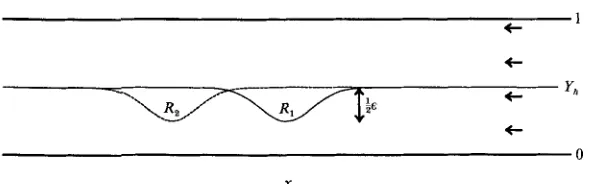
FIGURE 1. The geometry considered (after non-dimensionalization). The oncoming flow has speed 01 from right to left. The channel, assumed to be in a rapidly rotating frame of reference, is of constant width 1 with a step change in depth from a shallow shelf region in 0

<

y

<

Y,(x) to a deeper region in &(x) < y 6 1. The curve y = Y,(x) is shown as a solid line, and the vorticity contour dividing R ,

from R- is shown as a dashed line. In the cases described in detail in the text the shelf narrows smoothly by a fraction E in the neighbourhood of the origin. Region R , contains relative vorticity 1, region R, relative vorticity - 1.

It follows that the (non-dimensional) streamfunction $ satisfies the equation

Vz$ = 1 ( x E R ~ ) , ( 2 . 4 ~ )

V z $ = - l ( x E R ~ ) , Vz$ = 0 (otherwise),

(2.4b) ( 2 . 4 ~ )

where R, is the region 47

>

yh and x E R-, and

R,

the region y

<

Yh and x E R,. The boundary conditions are that @ = 0 on y = 0 and $ = a on y = 1.

The time evolution of the system is determined by the fact that the boundary between R- and R,, is %‘say, is a material contour and therefore advected by the local flow, i.e. if

%?={x(s,t); -oo < s < oo} ( 2 . 5 ~ )

then axlat = k x V$lx-x(s,t,, (2.5b)

where k is a unit vector in the vertical.

Equations (2.4) and (2.5) are sufficient to describe the evolution of the flow.

2.2. Linear theory

It is helpful to recall the linear theory for small disturbances to the basic state, perhaps induced by small deflections of the topographic step. We restrict attention to the case where the undisturbed position of the step is at the centre of the channel (i.e.

&(

f 0 0 ) = 0.5) since it is this case that will be considered later in the paper. The dispersion relation for waves on the vorticity contour, of wavenumber k and frequency o, is

o = -ak+;tanhik. (2 * 6)

The first term on the right-hand side represents the effects of advection and the second those of the q-contour. For a

>

the group velocity of all waves is negative (downstream), since the advection dominates, and no stationary (o = 0) wave of finite wavelength exists. For a

<

4

the group velocity of longer waves is positive (upstream), with the longest ( k = 0) waves having the largest upstream group velocity, and there is a finite wavelength for which waves are stationary.

Briefly, for small topographic displacements, the time evolution from an initial condition in which the q-contour lies along the topographic contour is as follows. For a

>

+

the initial perturbation in the q-contour is swept downstream and a steady stage

364 P. H . Haynes, E. R. Johnson and R. G. Hurst

waves, which propagate upstream, and shorter waves which propagate downstream.

As the displacement adjusts it builds a steady 'lee wave' pattern downstream in which the dominant wavelength is that which is stationary. The resulting steady-state pattern can therefore be highly asymmetric about the topographic displacement when the stationary wavelength is comparable to the lengthscale of the topographic perturbation.

2.3. Long-wave theory

We now consider the case where the topographic and contour displacements are finite and linear theory will not be accurate. The finite-amplitude behaviour is most tractable in the long-wave limit and we first consider possible steady states in this limit.

(i) Steady solutions

We assume that the x-scale of the topographic displacement is large compared with the width of the channel. One consequence of this assumption is that the y-coordinate of the q-contour %? is a single-valued function of x, which we denote by Y(x).

In the long-wave limit the x-derivatives can be neglected and (2.4a-c) therefore reduce to

$yy = 0 (0

<

y

<

min(Y,, Y ) ) , (2.6a)

?bYU = W ( Y -

r,)

(2.7b)

$YY = 0 (max(Y,, Y )

<

y

<

11, ( 2 . 7 ~ )

(min(Y,,

r> <

y < max(r,, Y ) ) ,

with $ = 0 on y = 0 and $ = a on y = 1.

These equations may be solved to give $(x, y) as

ay+8(1- Y ) " ( l - Y,y}y (0 < Y <

Y,),

oIy++{Y2- Y 2

?Jb-

1 ) ( Y < Y

<

11,

ay+;((I- Y y - ( l - yh)2)y (0

<

Y

<

0,

ay-;o,-Y,)2+;{Y;-Y2)(l-y) ( Y < y <

&),

$(x,y) = .y+ao,-Y)2++{Y~-Y2}(1-y)

( Y ,

<

y

<

Y ) , (2.8 a)

(2.8 b )

'I

if

&

<

Y , and

if

K

>

Y .

The steady-state solution is determined by noting that ~ ( x , Y ( x ) ) must be constant (and equal to aY, say) since there is no flow across the material contour '8, y = Y ( x ) .

It follows that Y(x) satisfies the implicit equation

= y2- y ;

Y - Y 2a ~

Y - 1 (2.9 a)

Y- Y

-2a-=(l-Y,)2-(1-Y)2 Y ( Y <

Y,).

(2.9b)

(ii) Time-dependent solutions

The long-wave theory extends directly to time-dependent flows. The same equations

(2.8a) and (2.8b) hold for $; the difference is that it is no longer required that $(x, Y ( x ) ) be constant. Instead the kinematical boundary condition at the q-contour requires that

A simple model of Rossby-wave hydraulic behaviour 365

0 0.2 0.4 0.6 0.8 1

.o

Y

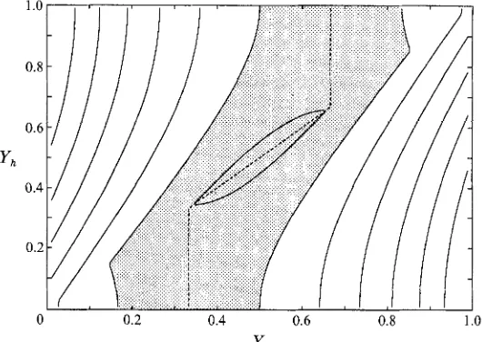
FIGURE 2. Contour plot of the long-wave speed c as a function of Y and

5

for a = 0.125. The contour interval is O.la and the highest-valued contour shown is 0.101. The region where c > 0 is shaded, The contour shapes and intervals would be the same for other values of a but the values would be different. In particular the long-wave speed is always a maximum at Y = =

t.

The zero contour therefore vanishes for a = 0.25 and the long-wave speed is then everywhere negative. To the left of the dashed line

&/a

Y > 0 and an isolated disturbance for which Y is anomalously large will therefore steepen to the right. Elsewhere such a disturbance will steepen to the left.

where the derivatives of $ are to be evaluated at y = Y(x, t). On substitution from

(2.8a) and (2.8b) it follows that

(2.11)

i

a y ay

at ax ax

- - { ~ ~ + ; [ 3 Y 2 - 2 2 - Y i ] - = (1 - Y ) Y 3

-++4[3(1- a y Y)2-2(1- Y ) - ( 1 - y h ) 2 ] } - ay = ( 1 -

r,)

Y-

a Y ,

( Y >

F-2,

( Y <

%).

at ax ax

This first-order hyperbolic equation expresses the propagation of long waves on the vorticity interface, the wave speed c being given by the coefficient of the x-derivative. Note that the wave speed is made up of two contributions, the first simply due to advection and the second to the Rossby propagation mechanism. The former is generally downstream (i.e. negative in the sign convention adopted here) for CL > 0, but

depends on Y and yh, and may under some circumstances be positive, even for a > 0.

The latter is equal to Y ( l - Y ) and is always upstream (i.e. positive).

The steepening behaviour of long waves also follows from (2.11). Note first that the form of the dependence of the wave speed on Y and

%

does not change as a function of a ; the varying part is independent of a. The steepening behaviour for all values of CL is therefore determined by the sign of ac/a Y , which is positive if Y

<

+(O <

Y ,

<

+) or

366 P . H . Haynes, E. R . Johnson and R . G . Hurst

indeed regions for which the wave speed is positive (i.e. upstream), but the shape of the contours, and the contour interval, is the same for all values of a.

3. Numerical integrations and interpretation

The evolution of the system was investigated by numerical integration of the unapproximated equations using the contour-dynamics (CD) algorithm described in the Appendix. Before considering specific cases it is useful to note the following simplifying convention. If the position of the topographic step is reflected about the channel centreline y =

i,

i.e. yh is replaced by 1 - yh, then the flow evolves with 1 - Y replacing Y. In particular, the steady-state configuration is unaltered under simultaneous reflection about both Y =

i

and yh =

i.

The following discussion and examples are thus simplified by describing only narrowing shelves where yh decreases smoothly with decreasing x from its upstream value to some minimum value in the neighbourhood of the origin x = 0. For localized topography yh then increases downstream with the shelf width far downstream returning to its upstream value. The symmetry of the problem means that the discussion applies directly to widening shelves also (though this would not be the case if the original ‘undisturbed’ configuration of the flow were not exactly symmetric). It is convenient to choose the origin x = 0 at the point of minimum shelf width and to introduce a measure of the fractional narrowing of the shelf,

For definiteness the discussion is further restricted to the case of a shelf occupying precisely half the channel width, i.e.

&++

as x + f co, but once again flow states for differing shelf widths are completely analogous to the present state and follow similarly. In this case the fraction by which the shelf narrows E = 1 -2&(0), (as indicated in figure 1). In all the cases examined numerically the topography is given by

E = 1 -

y , ( O ) / y , ( c o ) .

%(x)

=

8

1 - f2 exp [ - (x/L)21),

and the initial condition is Y(x,O) = Y,(x). The length L varies and will be given for each case as it is discussed.

It was found that the behaviour showed distinctly different forms in three different ranges of values of a. The first, a

<

a2 = 0.05448, we shall refer to as the weak subcritical regime, since the strength of the flow is weak relative to the appropriate measure of the vorticity jump and it is possible for waves to propagate upstream (for some values of Y and yh). In the second, a2 d a d a1 =

f,

the flow is stronger, but upstream propagation is still possible. We refer to this as the strong subcritical regime. Finally, in the third regime, LY > aI, the flow is stronger still and no upstream propagation is possible. We refer to this as the supercritical regime. The values for a1

and a2 are for the case where the topographic step and, initially at least, the potential vorticity contour both lie in the centre of the channel far upstream and downstream of the topographic perturbation. For other upstream configurations the values of L Y ~ and

a2 will be different, but a similar set of regimes will exist. We now describe the regimes one by one.

3.1. The weak subcritical regime

(LY

d a2 = 0.05448)

For steady flow in the long-wave limit the position Y ( x ) of the streamline &c, Y(x))

A simple model of Rossby-wave hydraulic behaviour 367

1

.o

0.8

0 6

Yll

0 4

0.2

0 0 2 0 4 0.6 0.8 1

.o

Y

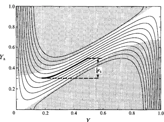
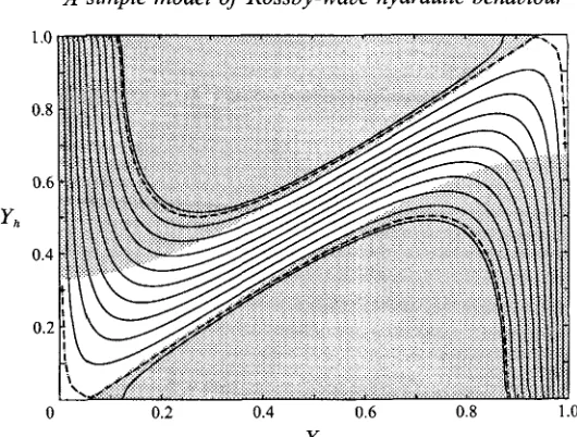
FIGURE 3. Graphs relating the position Y(x), of the streamline @(x, Y(x)) = Y dividing low-potential- vorticity fluid in y > Y(x) from high-potential-vorticity fluid in y < Y(x), to the local position %(x)

of the step change in depth, according to the steady long-wave solution (2.9a, b). The flow regime is

subcritical, with a = 1 / 6 r % is plotted as a function of Y for values of Y ranging from to 0 to a at intervals of 0. la. Part of the curve for Y =

h

is shown in bold and discussed in detail in the text. The shaded regions bounded by bold lines show those values of Y and % for which there is reversed flow (discussed in detail in 94).

plotting

5 as a function

of Y. Figure 3 gives, for 01 = 1/611 a number of curves

corresponding to different values of Y. Note the general property of such diagrams that in regions where the gradient a&/aY of the steady state curves is positive, the flow is subcritical (long waves propagate upstream) and in regions where the gradient is negative the flow is supercritical.-(This can be verified directly from (2.9a), (2.9 b ) and

(2.1 . l).) , I

Consider first the partially bold curve in figure 3 corresponding to Y = 0.501, the value of Y for the steady long-wave solution to join smoothly to unperturbed flow far upstream. This curve has a turning point where

%

is a minimum as a function of Y,

corresponding to a critical narrowing of the shelf, when E = el, with el = 0.3911 (for this value of a). Provided E < el, i.e. the shelf narrows less than the critical amount, following the bold curve gives the change in Y as

& varies. With

x decreasing from large values,

& decreases from and hence

so too does Y but more rapidly, so that

Y <

%

and the dividing streamline deviates more than the perturbation to the step: some low-potential-vorticity fluid mounts the shelf. As yh passes symmetrically through a minimum value at the origin so too does Y, and as

%

increases downstream the point ( Y ,

&)

retraces the bold curve returning eventually to

(i,

!j) Since the gradient of the bold curve is positive the free long-wave speed is greater than the imposed flow speed and the flow is subcritical throughout. We therefore describe this regime as

' symmetric subcritical '.

368 P. H . Haynes, E . R. Johnson and R. G. Hurst

- t I " " I " " I " " I " " I " " I " " 1 " " 1 " " 1 " " 1 " " I " ~ ' I " ' ' I '

X

-4 - 2 0 2 4 6

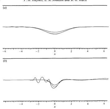
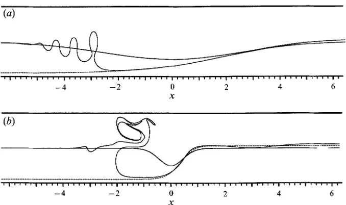
FIGURE 4. Contour-dynamical integrations of the full equations of motion for u = 1/6n and E = 0.25. Here E < z 0.39 and the flow is subcritical. In these and later diagrams the edge of the shelf step is shown as a thin continuous line and position of the material contour W at various times by thicker continuous lines. Steady solutions derived from the long-wave limit are dashed curves. ( a ) The material contour at t = 102 and L = 42/2/71, The flow deviates from the steady long-wave solution solely in the presence of a train of short lee waves of almost vanishingly small amplitude. (b) For a shorter obstacle ( L = 2 / x ) with scale more closely comparable to the wavelength of the standing wave. At t = 42 a stronger lee-wave wake begins to emerge.

The sole difference is the presence of a very small-amplitude lee-wave wake downstream of the constriction. The dominant wavelength within the wake is that of the unique small-amplitude wave with zero phase speed. This wave has finite wavelength equal, from (2.6), to 0.6667 and is of course absent from the long-wave limit. It is only weakly excited as its wavelength is only about one quarter of the length of the topographic perturbation. Figure 4@) shows a CD integration at time t = 42 for the same oncoming flow ( a = 1/6z) and constriction width (e = 0.25) but for the much shorter scale L = 2/n. The obstacle scale is far more closely comparable to the wavelength of the standing wave (determined by 01 alone) and hence a stronger lee-wave wake is beginning to emerge. For small 8 the equations of motion can be linearized about

A simple model of Rossby-wave hydraulic behaviour 369

Y

-15 - 10 - 5 0 5 10

X

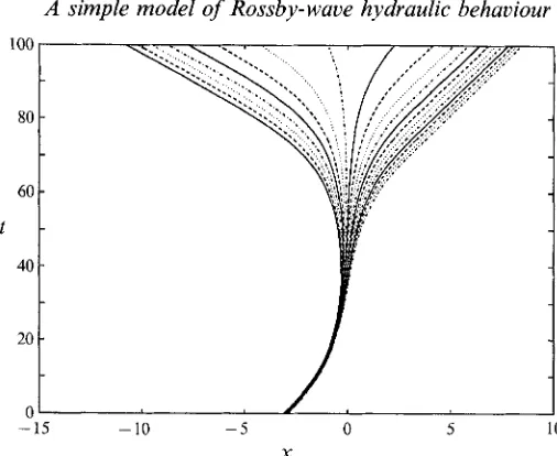
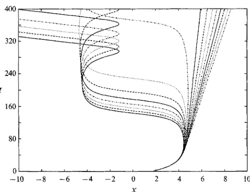
FIGURE 5. Characteristic integration of the long-wave equation as in figure 4 for L = 82/2/n: and the same flow strength a = 1/6z but with an increased narrowing, B = 0.5. The set of characteristics have been chosen to start close together and to fan out from the region of the control point at the origin.

If the shelf narrows to precisely the critical amount, i.e. E = el, then the long-wave speed vanishes at the narrowing. For narrower constrictions, E > el, the bold curve in figure 3 no longer yields a solution. A unique smooth solution for E

>

el can however be deduced through analogy with open-channel flow, by requiring that the flow is determined by the condition that the long-wave speed vanishes at the narrowest point of the shelf. In terms of the solution curves shown in figure 3, this selects the unique curve that attains its minimum & as a function of Y at the narrowest point of the shelf. Such a curve corresponds to a value of 'Y smaller than 0.5a and therefore represents a partial blocking of the flow on the shelf. The slopes of the curves in figure 3 show that the large-time solution may be determined by information propagating away from the control at x = 0. In particular, steady upstream values of Y (where the flow is subcritical) follow by requiring Y to increase along @ = Y as

Y,

increases upstream from the control, and the downstream values of Y (where the flow is supercritical) follow by requiring Y to decrease as

&

increases downstream from the control. Upstream and downstream influence therefore appear simultaneously A consistent picture emerges from the long-wave characteristic integration shown in figure 5, with

L = 81/2/n: and E = 0.5, obtained by initializing a set of closely spaced characteristics in a region from which they subsequently diverge. The characteristic passing through any fixed positive or negative x at sufficiently large time t can be traced back to a region arbitrarily close to x = 0, showing that the flow may indeed be controlled at the origin. Note however that if characteristics are initialized at a wider range of points then some intersect downstream of the constriction (x c 0) at times t

>

35 showing that Y

370 P . H . Haynes, E. R. Johnson and R . G . Hurst

-4 -2 0 2 4 6

A

(b)

_---_-_--.___.________

-

-

v

I ~ ~ ~ ~ l ~ ~ ~ " " ~ " ~ ~ ~ " ~ ~ ~ " " ~ ~ I ~ ~ ~ ~ I ~ ~ ~ ~ I ~ ~ ~ ' I " " I " " I " " I '

- 4 -2 0 2 4 6

X

FIGURE 6. Contour-dynamical integrations for the same flow strength and narrowing (a = 1/6n, E = 0.5) as figure 5. (a) For L = 81/2/n the flow at any fixed x rapidly approaches the dotted steady long-wave solution. This steady solution is joined to undisturbed flow far downstream by a down- stream propagating jump in the form of an undular bore (absent from the long-wave integration). The rear face of the bore shows here, at t = 78, fluid being pinched slightly into an eddy. This is more pronounced for the shorter narrowing in (b) where L = 2/n and by t = 45 an anticlockwise eddy has formed at the downstream propagating jump between controlled flow and undisturbed flow.

the leading edge of the upstream propagating disturbance is expected to take the form of a rarefaction. Again this is consistent with the results of the CD integration.

For smaller L the behaviour is more complex, with positive vorticity shed as an eddy in the deep flow as in figure 6 ( b ) , where e and a are unchanged but L = 2/n. Figure

6 ( b ) includes for comparison the steady controlled solution derived from figure 3,

showing that even for short obstacles the steady long-wave limit accurately predicts the upstream influence and the transition of the flow from upstream to downstream of the centre of the obstacle.

The behaviour described here, with the control at the origin, is typical of all sufficiently slow flows (a small) for which E exceeds el. (Figure 9 below gives values of the critical narrowing el as a function of the flow strength a.) For small a it can be shown that

(3.1)

and therefore el increases relatively slowly towards 1 as a decreases.

The decreasing value of Y for the material contour %? in the steady flow indicates that the flow on the shelf becomes progressively blocked with increasing e. Indeed, the steady long-wave theory predicts that under some circumstances reversed flow, and therefore recirculation, occurs. This is examined more closely in 94.

el = 1 - 2(2a)f

+

O(a),

3.2. The strong subcritical regime (a,

<

a

<

al)

A simple model of Rossby-wave hydraulic behaviour 371

0 0.2 0.4 0.6 0.8 1

.o

Y

FIGURE 7. As figure 3, but here for the critical value a2 = 0.05448 of the flow strength a. Again graphs are plotted for Y = 0, O.la,

...

0.9a, a (solid curves). The dashed curve is for that value of Y corresponding to the hydraulically controlled flow for the largest possible narrowing of E = 1, where the shelf narrows to zero width at the origin. The fact that the gradient of this curve is zero on

r,

= 0.5 indicates that the speed of long-wave perturbations decreases monotonically upstream to vanish at x =

+

CT).

Y

FIGURE 8. As figure 3, but here for faster flow with a = 1/3a. Here the dashed curves correspond to those values of Y for which the gradient of the graphs (and therefore the wave speed) vanish with

Y, = 0.5 and those for which the gradient vanishes on

r,

= 0 or 1 and which might therefore represent states that are hydraulically controlled with E = 1. In the case of interest, where

5

decreases from its upstream value, the flow pattern for sufficiently large E is eventually determined by the bold portion

of the curve marked AB. The streamline displacement Y increases as the shelf narrows and

r,

decreases, before returning symmetrically towards its undisturbed value as

r,

increases downstream. There is then the possibility of a jump from the part of this curve marked AC to that marked DE. Unlike the controlled subcritical flow the displacement of Y from

+

in the far field, the amount of

upstream influence, is determined solely by the value of a and is independent of E. It takes its

372 P . H . Haynes, E. R. Johnson and R . G. Hurst

Symmetric supercritical

Controlled from

0 0.1 0.3 0.4 0.5

o.2

t

t

CL

a, 011

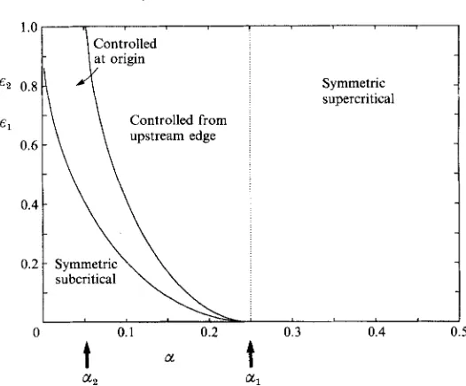
FIGURE 9. The various long-wave flow regimes determined by the flow strength a and the fractional shelf narrowing e. For large shelf step heights or slow flow (a < a,) the flow is upstream-downstream symmetric and subcritical for small narrowings (0

<

E < el), and asymmetric controlled at the origin for more extreme narrowings (el < e

<

1). For moderate step heights or flow speeds (a, < a < a,) the flow remains symmetric subcritical for e < el. The behaviour for more extreme narrowings splits: for

el < E < e2 the flow is asymmetric and controlled as for larger a but for the greatest narrowings ( E , < e) the flow is supercritical and controlled from the upstream edge, and the upstream conditions having been modified by a fast upstream propagating transient. For low shelf steps or strong flow a >

i)

the flow is supercritical with no upstream influence.

In the present example of a shelf occupying half the channel width a, = 0.05448. As

described above, for cr: d az the flow takes two forms depending on whether E is greater

or less than el. For 01

>

a, an additional form appears. Figures 7 and 8 give the curves

of

& as a function of

Y analogous to figure 3 but for faster flow, for a = a2 and a = 1/3n, respectively. In figure 8 the curve with zero long-wave speed far upstream

( yh = 0.5) is marked partially dashed and partially bold. Since a > a, this curve has a minimum of

& as a function of

Y. Denote the critical narrowing corresponding to this minimum by eZ. Here el = 0.1868 and e2 M 0.3766. As for 01

>

aZ, if 0

<

E

<

el the flow is subcritical everywhere, whilst if el d E < eZ the flow may be asymmetric, controlled at the origin (i.e. the narrowest point of the shelf). For E

>

E~ the curves corresponding to flow controlled at the narrowest point do not connect via subcritical flow to any upstream flow (where of necessity yh =

OS),

and so either of the above flow forms is possible. The variation of eZ with a is also shown in figure 9.

In order to understand what form the flow might take in this case it is useful to consider the wave speed, c( Y, yh), for the shelf width far upstream, i.e. for

&

= 0.5. For upstream propagation of disturbances, c( Y, 0.5)

>

0, which occurs only for those curves crossing yh = 0.5 between Y = 1 -

Y,

and Y =

Y,

where Y, is the unique contour displacement for which c(

Y,,

0.5) vanishes and

Y,

>

0.5. It does not seem possible for

A simple model of Rossby-wave hydraulic behaviour 373

J

-10 -8 -6 -4 - 2 0 2 4 6 8 10 X

FIGURE 10. Characteristics of the long-wave equations for CL = 1/3n and a topographic perturbation of the form Y,(x) = 0 . 5 - 0 . 2 5 ~ 0 ~ ~ ( 1 r ~ x / 3 2 ) (for 1x1 < 16/1r) and Y,(x) = 0.5 (for 1x1 > 16/1r). Thus, according to the definition (3.1), E = 0.5. The fan of characteristics shown determines the ‘upstream- edge ’ controlled solution. The characteristics on the downstream side of the topographic perturbation indicate the possibility of a short-lengthscale feature allowing a transition from the ‘ upstream-edge- controlled’ flow to the downstream supercritical flow. There is also a fan starting somewhat to the left of that shown which initially resembles the fan in figure 5. However, the upstream propagating characteristics of this fan subsequently turn downstream and so cannot affect the upstream flow.

For e

>

e2 the solution joining the flow in the neighbourhood of the constriction to the upstream flow is determined uniquely by the values of ( Y ,

&)

given by the curve

AB. As

Y,

decreases from 0.5 at A, Y increases, passing through a maximum value as

Y,

passes through its minimum at the origin. As

Y,

increases downstream towards 0.5,

Y decreases. Once Y, has increased so that the shelf displacement is less than ez, it is possible for the solution to jump from the bold curve between the points C and A to the portion of the dashed curve with negative slope between the points D and E.

Since the slope of the bold curve is negative throughout, the hypothesized steady flow is supercritical, controlled from the upstream edge of the obstacle, but with upstream influence that must be caused by the initial transients. Indeed, initially the configuration of the characteristics is similar to that in the hydraulically controlled case (as seen, for example, in figure 5). However, unlike that case, there is a later reversal of some of the characteristics that are initially propagating upstream. This leads to control by a second fan of characteristics adjacent to the unique characteristic that separates those that ultimately propagate downstream from those that ultimately propagate upstream. For a topographic perturbation of infinite width, as has been considered previously, the separatrix has x-tm as t+m, but with the gradient dx/dt increasing indefinitely. For a topographic perturbation with compact support, and therefore vanishing for x

>

xu, say, the separatrix tends to x = xu as t increases.

3 74 P . H . Haynes, E. R. Johnson and R . G . Hurst

(b)

4_

i

i

I " " l " ' l l " " l " ' ~ 1 " " 1 " " 1 " " 1 " " I " " I " " I ' " ' I " ' ' I '

-6 - 5 -4 - 3 -2 -1 0 i 2 3 4 5 6

X

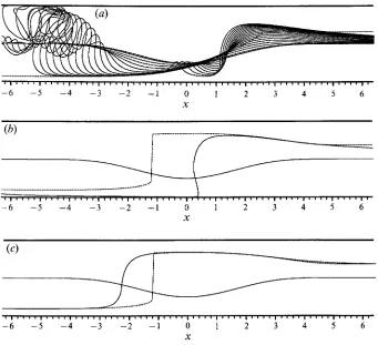
FIGURE 1 1. Contour-dynamical integrations for the cosine topography and upstream flow of figure 10. (a) The material contour W at unit time intervals from t = 0 to 18. The dashed curve gives the steady long-wave solution obtained by assuming that the flow is controlled at the narrowing. This solution extends only a finite distance upstream before the associated long-wave speed vanishes with dY/dY,+co and the predicted material contour W becomes vertical. Initially the flow develops towards supercritical controlled flow downstream of the narrowing with the supercritical flow rejoining undisturbed flow through a downstream propagating jump and a positive eddy that is also advected downstream. (b) At later times the material contour W steepens upstream of the narrowing to form, by t = 26.5, a jump that begins to move downstream. The dashed curve is the steady long- wave solution obtained by assuming that the flow is controlled from the upstream edge of the constriction and assuming that the flow jumps from off-shelf to on-shelf at the first opportunity. (c)

By t = 77.5 the jump has stopped moving, giving a steady flow that follows closely first the off-shelf upstream-edge-controlled solution, then jumps downstream of the maximum constriction onto the on-shelf branch.

the wave speed must be zero at both ends of the obstacle. The characteristics then return part of the way over the obstacle, now with the behaviour corresponding to the subcritical branch AD in figure 8, and then turn again to run downstream off the obstacle, corresponding to the supercritical branch DE. The crossing of characteristics predicted on the downstream part of the obstacle tends to indicate that the 'upstream edge controlled' solution corresponding to the curve AB will not hold over the entire obstacle and again suggests that there may be a transition from the branch AB to the branch DE somewhere on th downstream slope of the obstacle.

A simple model of Rossby-wave hydraulic behaviouv

1 0

0 8

0 6

375

0 0.2 0.4 0.6 0.8 1.0

Y

FIGURE 12. Curves relating Y to Y, as in figure 3 but here for the critical value a1 = 0.25 of the flow strength a. The bold curve representing the supercritical solution with zero long-wave speed far upstream passes through Q,;). The flow for all obstacle heights is symmetric supercritical flow with no upstream influence.

downstream of the obstacle are resolved as a developing positive vorticity eddy, allowing the downstream connection from supercritical to undisturbed flow. The evolution towards the hydraulic steady state eventually ceases as fluid piles up upstream of the constriction and the returning contour overshoots. The increasing complexity and length of the contour precludes direct longer time integrations. The integrations were however continued from the last available position by smoothly joining the downstream supercritical controlled flow to the undisturbed material contour, eliminating the need to resolve the motion of the shed eddy. Varying the time and position of this smoothing made no perceptible difference to the evolution of the flow in the neighbourhood of the constriction. The contour %2 continued to steepen immediately upstream of the origin eventually coming arbitrarily close to the sidewall as shown in figure 11 (b), before moving downstream to take up the seemingly steady shape of figure 11(c). This steady solution shows a rapid transition from off-shelf to on-shelf flow downstream of the maximum constriction. The contour shapes upstream and downstream of this transition agree closely with the forms for the two supercritical solution branches predicted by the long-wave theory.

The flow patterns described in this section are typical of the strong subcritical flows where a2

<

a < al. As flow speeds increase and a increases towards a1 the separation of the evolution into a distinct intermediate stage of flow controlled at the constriction and a final supercritical flow with modified upstream conditions blurs.

3.3. The supercritical regime (a 2 al)

With increasing flow speeds or shallower steps the range of e for subcritical and constriction-controlled flow become smaller, with both E, and e2 vanishing simultaneously at a = a1 = 0.25 (figure 12). The flow at a = a, is determined by the unique bold curve representing undisturbed flow far upstream passing through ( Y ,

5 )

376 P. H . Haynes, E. R. Johnson and R. G . Hurst

Y

FIGURE 13. Curves relating Y to as in figure 12 but here for the more rapid flow of cc = l / n > ccl. The bold curve passing through

(i,

+) with negative slope represents steady long-wave solutions formed by long waves being swept downstream at finite speed to leave supercritical, symmetric flow with no upstream influence.

I " " I ' " ' l " ' ' l " ' ' I " ' ' , l " ' l ' ' " l " ' ' I ' " " ' ' " I ' ' " I ' ' ' ' ~ '

-6 - 4 - 2 0 2 4 6

X

FIGURE 14. Contour-dynamical integrations for cc = 1/n, E = 0.5 and L = 8/n at times t = 15 and 23. The inclusion of the short waves in the full calculation removes multivaluedness predicted by the corresponding long-wave characteristic integration. The flow rapidly approaches symmetric subcritical flow that is undisturbed away from the narrowing. The dashed line shows the steady solution predicted by long-wave theory.

A simple model of Rossby-wave hydraulic behaviour 377

4. Reversed flow

It is implicit in the steady-state analysis leading to figure 3 (and its equivalents for different values of a) that the potential vorticity takes only two values across the flow. It is clear that this condition is most likely to be satisfied if the flow is everywhere in the negative x-direction (so that, for example, the potential vorticity debris arising from the formation of small-wavelength features is swept downstream away from the topographic obstacle).

The requirement for no reversed flow has also been noted in Pratt & Armi (1987) in the context of models where the potential vorticity varies continuously across the flow and the nonlinear steady solution follows from the functional relation between the potential vorticity and the stream-function, set by the assumed upstream conditions. Reversed flow, in the sense that all streamlines no longer connect smoothly to the upstream flow then invalidates the nonlinear solution. In the case studied here the requirement for the validity of the nonlinear steady solution is less severe because streamlines that lie fully within regions where the potential vorticity is homogeneous play no dynamical role. However, even in cases where it does not disrupt the nonlinear solution, reversed flow is still of interest because of the implications for tracer transport.

Equations ( 2 . 8 ~ ) and (2.8 b) show that the velocity in the downstream direction takes its minimum value Umin in the region neighbouring one of the channel walls, with

Umin = a+f(Y2- Y 2 h ) ( Y <

Y,>,

(4.1 a)

Um,,=a+f((l-Y)2--(1-&)2) ( Y >

6).

(4.1 b)

It follows that there is the possibility of reversed flow if a

<

f and the region of a

steady-state diagram such as figure 3 in which it occurs is given by

Y 2 < Y;-2a ( 4 . 2 ~ )

and ( 1 - Y>2

<

( 1 - r,>"2a. (4.2b)

Note that these regions enlarge as a decreases. It follows that almost all possible steady states include some reversed flow as a becomes very small and that hydraulically controlled states include reversed flow downstream of the obstacle if the supercritical extension of the bold curve in figure 3 to

&

=

+

(or its analogue for other values of a> enters the regions defined by ( 4 . 2 ~ ) or (4.2b). This turns out to be the case for all possible such states for given a if a < a, with a, = 0.1 11 1.

The streamlines for the steady flow according to long-wave theory for the configuration in figure 6 ( a ) are shown in figure 15(a). Upstream propagating waves have modified the oncoming flow so the greater part of the downstream mass transport is off the shelf. This deep water mounts the shelf at the constriction to form a rapid jet.

A stagnation point appears in the neighbourhood of the constriction and a recirculating eddy forms outside the jet. In the flow configuration being studied here, with piecewise- constant vorticity taking only two values, the reversed flow invalidates the solutions already derived only if it draws the contour back from downstream over the obstacle. For the cases being discussed in this subsection there is no evidence that this occurs, either from figure 15 (a) for a very long topography, or for shorter topography, as may be seen from figure 15 (b), which shows streamlines calculated from the CD integration corresponding to figure 6(b). The latter show that at large but finite times the eddy terminates downstream and thus draws no fluid from x = - co. The fluid within the elongating eddy thus originates locally as assumed in the long-wave analysis.

378

P.

H . Huynes, E. R. Johnson and R.

G.

H u n t

-4 - 2 0 2 4 6

X

- 4 - 2 0 2 4 6

X

FIGURE 15. Streamlines for the same flow strength and narrowing (a = 1/6n, E = 0.5) as in figures 5

and 6. (a) The steady long-wave solution with L = 8 2 / 2 / x . Flow over the shelf is almost blocked upstream, with off-shelf deep flow mounting the shelf at the narrowing. This combines with recirculating flow downstream to form a strong downstream coastal jet. (b) The full CD solution for

L = 2/n at t = 45. The recirculating region downstream of the narrowing is terminated by the downstream propagating jump and eddy. Fluid in the recirculating region originates upstream. (c) The steady long-wave solution with L = 8 2 / 2 / x and E = 0.9, showing reversed flow upstream.

There may also be reversed flow upstream. For each a in the weakly subcritical regime this occurs for some value of E greater than the critical value el, but less than 1. Figure 15(c) shows the streamlines for an example, with a = 1/6n and E = 0.9. For small a the condition that there is reversed flow upstream is that

E > 1-2(22/2-l)a+O(a2). (4.3)

In the new 'upstream edge controlled' regime there is again the possibility of reversed flow. It can be shown from (2.9u), (2.9b), ( 4 . 2 ~ ) and (4.2b) that the upstream supercritical flow is reversed if a

<

4 4 2

-:

= 0.082 11. For g 4 4 2 - 5) < a

<

0.1479 the flow must be reversed somewhere on the obstacle. Lastly, for 0.1479

<

a <

4

the long-wave solution predicts no reversal, either upstream or over the obstacle.

Figure 16 shows recirculation patterns in flows controlled from the upstream edge

A simple model of Rossby-wave hydraulic behaviour 379

-6 - 4 -2 0 2 4 6

X

-6 - 4 -2 0 2 4 6

FIGURE 16. (a) Streamlines for the steady long-wave solution corresponding to figures 10 and 11. An isolated eddy at the constriction holds the flow off the shelf until a jump at the downstream edge of the eddy where the entire oncoming flow mounts the shelf. (b) Streamlines from the steady contour- dynamical solution showing details, missing from the long-wave solution, of the eddy edge and the transition region. The close alignment of the material contour V (shown as a second dashed line) and the independently calculated streamlines confirms that the flow is steady.

Figure 16(b) shows the flow pattern from the corresponding asymptotically steady CD integrations. The inclusion of the short-wave terms resolves the details of the flow at the transition but has negligible effect elsewhere. With increasing flow speed the recirculating region extends further downstream and the jump weakens, vanishing completely when a exceeds a,. The flow is then symmetric with neither upstream nor downstream influence. The eddy at the constriction blocks the shelf almost completely, forcing the bulk of the oncoming flux into the deeper part of the channel both upstream and downstream.

Reversed flow is, of course, possible in hydraulically controlled cases too for a1

<

a

<

a2. _As remarked earlier the downstream supercritical flow is then always reversed if a

<

0.1 1 1 1 and it may also be shown that it is reversed for sufficiently large topography (but sufficiently small that the upstream supercritical regime is not entered) if a

<

0.1248. In the upstream subcritical flow there is no reversal if a

>

$(41/2 - 5 ) =

0.082 11. It follows then that for 0.1248

<

a < 0.25 there is no flow reversal in any part of the hydraulically controlled regime. This result in itself would be a strong indication that hydraulically controlled flows are realizable in practice (although the CD integrations have in fact shown that the occurrence of reversed flow does not necessarily invalidate the hydraulically controlled solutions).

5 . Conclusion

5.1. Summary

In this paper we have analysed what is arguably the simplest system that supports Rossby-wave behaviour and have presented examples of flows that evolve to a hydraulically controlled steady state. Similar states have been postulated in the Rossby

380 P . H . Haynes, E. R . Johnson and R. G . Hurst

wave regime by Hughes (1989 and references therein), Pratt & Armi (1987), Pratt (1989) and Woods (1993) from steady-state analysis of different, often more complex, models. We have supported the steady-state analysis by consideration of the time- dependent problem, including full numerical integration, and have shown that asymmetric states are possible, even in regimes that seem well outside that of long-wave theory. We have also identified a new hydraulic behaviour where the flow is controlled from the upstream edge of the obstacle. The behaviour of the system is summarized in figure 9. Whilst the model that we consider is not intended to represent any particular oceanographic context, it has much in common with models of coastal currents, and of large-scale mid-ocean currents with localized potential vorticity gradients (such as those considered by some of the abovementioned authors) and more realistic models of either can be expected to display similar behaviour.

5.2. Relation to open-channel hydraulics

The behaviour of the system is in many ways similar to that found in the more familiar case of hydraulically controlled open-channel flow.

One difference is the existence, in the system that we have studied, of an ‘upstream supercritical’ regime, in which the flow is initially subcritical, but disturbances propagate upstream to change the flow in such a way that the flow over the obstacle is supercritical, with the wave speed vanishing in the upstream flow. The usefulness of the graphs of

& against

Y at constant Y mirrors that of graphs of specific energy in open-channel flows. However, figure 9 shows that once the form of the solution has been determined discussion of the general properties is more straightforward taking the topography to be given and considering the effects of varying flow speed. Then for all narrowings discussed here flow states pass with increasing flow speed from symmetric subcritical flow through flow controlled at the origin to supercritical flow with upstream influence and finally purely supercritical flow with the speed a for the various transitions decreasing with increasing E (except for the final transition which occurs at

a =

4

for all 6 ) .

In the open-channel case it is possible to characterize fairly completely the behaviour as a function of obstacle height and oncoming flow speed (see e.g. Baines 1987). This includes cases where there is a downstream propagating hydraulic jump, and others where the downstream hydraulic jump occurs at some position on the obstacle. In the system under consideration in this paper, it is clear that a phenomenon akin to a hydraulic jump may occur, for instance when freely propagating long waves steepen. Pratt (1989) mentions this possibility, including a possible example in a laboratory experiment. It is possible to consider the analogue of hydraulic jumps in the system under consideration, with a localized change in the position of the vorticity contour, and to derive the propagation speed as a function of the positions of the vorticity contour on either side of the jump. However it is not particularly clear that such simple models of hydraulic jumps in this context are as robust as they appear to be in open- channel flow. If they are, then knowledge of their properties (e.g. propagation speed as a function of amplitude) might be sufficient to characterize the behaviour of flow over long topography rather completely. But one reason for thinking that they might not be

so robust is that the local dynamics of the jump might well lead to vorticity ‘debris’ (e.g. as in figure 6 b ) which is subsequently advected away, thereby changing the state of the flow away from the jump. If this was the case, then even if simple models could be formulated they would surely have to be based on the results of thorough numerical experimentation.

A simple model of Rossby-wave hydraulic behaviour 38 1

been demonstrated by Pratt (1983). In the Rossby-wave context, recent CD integrations for initial value problems over isolated topography reported in Davey, Hurst &

Johnson (1993) show that for some parameter values the final state differs for differing speeds of start-up. The numerical results presented here are for the particular case of impulsively started flow and the evolution in some cases could possibly be altered by switching on the flow more gradually.

Again motivated by the analogy with open-channel hydraulics, one might ask whether there is any possibility of the transport through a system being hydraulically controlled, as in flow over a weir. The most obvious analogy would be a case where the upstream potential vorticity distribution was determined, but the net transport through the system was unknown and fixed by the requirement of a critical condition at a topographic obstacle. However, one might generalize the idea of hydraulic control to a forced system, e.g. a current system forced by wind stress. One might most straightforwardly represent such a forcing in the model that we have considered above by applying a body force that is independent of y , and therefore leaves the potential vorticity distribution unaffected by changes the integrated flux a. It is clear that, in the limit where the forcing was locally weak, so that the hydraulic solutions derived above were valid over the obstacle, but important in the x-integrated sense, there would be the possibility of the transport in the system being determined by the balance between the wind stress and the topographic drag associated with the hydraulically controlled state. Of course, the notion of topographic control of wind-forced currents is not new, but what is being raised here is the possibility that the topographic control is specifically a hydraulic one, distinguished by a subcritical to supercritical transition over the topographic obstacle, and with the control being effected at one particular location on the obstacle (which may have a complex and non-localized form). It is thus to be distinguished from control through the drag resulting from multiple-lee-wave trains, for example.

5.3. Applications

An obvious oceanographic example that might show hydraulic effects is the Antarctic Circumpolar Current. Davey (1978) has presented models where the transport for a given forcing is determined by topographic effects and Pratt (1989) has already considered the possibility of hydraulically controlled states on this current. The possibility arises that net transport in the Antarctic Circumpolar Current is determined by hydraulic control at one or two locations.

The same possibility would presumably apply to the case of coastal currents. Some of the flow patterns discovered are of particular interest in this context. That shown in figure 15, for example, shows that the flow on the shelf may be almost completely blocked, with the transport confined to a narrow coastal jet. The existence of the recirculating eddy offshore presumably has implications for the dispersal of pollutants in such flows.

5.4. Dispersive effects

382 P. H. Haynes, E.

R.

Johnson and R. G . Hurst

that on which we have concentrated here, where the vorticity contour and the topographic contour coincide in the initial upstream and downstream states. The resulting equation takes the form

where the various quantities are defined by Y = Y,+py,

&

= Y,+pu2y,,

X =

pix,

T = pit and p A = c, where c is the long-wave speed corresponding to Y =

&

= Y,,

with p being a small parameter.

The authors are indebted to Dr D. G. Dritschel for allowing them the use of his contour-dynamics code and to Dr J. Nycander for his careful reading of an earlier version of the paper. P. H. H. wishes to acknowledge conversations with Drs P. G.

Baines and P. B. Rhines and financial support in the form of a Royal Society Meteorological Office Research Fellowship in Dynamical Meteorology. R. G. H.

acknowledges support from the Science and Engineering Research Council and the Meteorological Office through a CASE Studentship.

Appendix. Numerical solution

The full evolution equations may be integrated by the method of contour dynamics. This technique has been widely used since the early studies of Deem & Zabusky (1978) and has proved to be highly efficient in investigations of the development of piecewise- constant-vorticity flows. The problem is effectively reduced to one dimension and all computational effort is concentrated on tracking the boundaries of the constant- vorticity regions.

The streamfunction, $, may be found by the use of the Green's function for equation (2.4) (e.g. a simple extension to Lamb (1932, $156)) to be

$(x, y ) = ay

+

5

log

[

sinh2

("'"

2

"'I)

+

sin'

(

'0, -Yo)

)]

'

dx, dy,

k=1,2 2'

-

C

5

JJR, log

[

sinh2

(ncx

2

",I)

+

sin2

(

)]

_{'dx, dy,, (A 1)}

k=1,2 2n

where

R,

are the regions of non-zero relative vorticity defined in (2.4) and wk = (- l)"-l. By Green's theorem, (A 1) gives the horizontal velocities as

U(X,Y> = (u, v) = (-a, 0)

-

C

5

1

log

[

sinh'

(

'("

2

".')

+

sin2

(""

~ y o ) ) ~ ( d x o , dy,)

k=1,Z2' aR,

+

: ,

,

2

la,,

log

[

sinh'

("'"

2

"O')

+

sin2

(""

yo))r( - dx,, dy,), (A 2)