Feature Subset Selection in Large Dimensionality Micro array using Wrapper Method: A Review

Feature Subset Selection in Large Dimensionality

Micro array using Wrapper Method: A Review

Binita Kumari

, Tripti Swarnkar

Department of Computer Science,

Department of Computer Applications, ITER, SOA University

Orissa, INDIA

Abstract— The high dimensional feature vectors of microarray impose a high dimensional cost as well as the risk of overfitting during classification. Thus it is necessary to reduce the dimension through ways like feature selection.

In this paper, we make the people aware of the various techniques of feature selection.

Keywords— Microarray, Feature Selection, Classification.

I. INTRODUCTION

The DNA microarray [1] technology is providing great opportunities in reshaping the biomedical science. A systematic and computational analysis of microarray datasets is an interesting way to study and understand many aspects of underlying biological process. Parallel to these technological advances has been the development of machine learning methods to analyse and understand the data generated by this new kind of experiments. The analysis involves class prediction (supervised classification), regression, feature selection, principal component analysis, outlier detection, discovering of gene relationships and cluster analysis (unsupervised classification) [1,3].

Feature selection can be applied to both supervised and unsupervised learning; we focus here on the problem of supervised learning (classification), where the class labels are known beforehand.

A DNA microarray is a multiplex technology which is being used in molecular biology which consists of an arrayed series of thousands of spots of DNA which are called features. Microarray technology is used to study the expression of many genes at a time. The high dimensional [2,5] feature vectors of microarray data often impose a high computational cost as well as the risk of “overfitting” at the time of classification. Thus it is necessary to reduce the dimensionality through ways like feature selection.

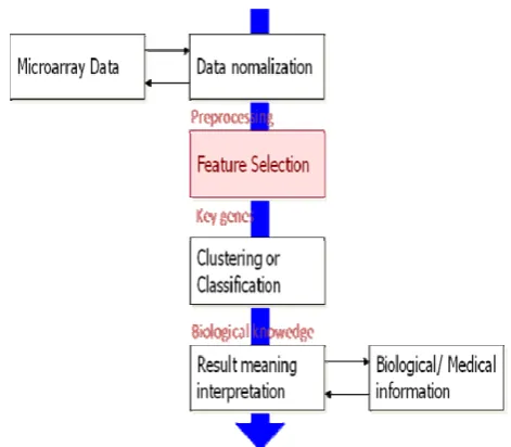
A microarray chip or data can be analyzed as shown in figure 1.First the microarray dataset is normalized so that there are no missing values and the data is scaled between a specific range. Then feature selection is done as a result of which we get the key genes. Then the classification or

clustering is done and the output is interpreted to get the required biological information

Fig.1 Microarray chip analysis

The selection of relevant features and elimination of irrelevant ones is a great problem. Before an induction algorithm can be applied to a training dataset to make decisions about test cases, it must decide about which attributes to be selected and which to be ignored.

Irrelevant features increase the measurement cost, decrease the classification accuracy and add to making the computation complex. Obviously, one would like to use only those attributed that are relevant to the target concept.

II. REVIEW OF EXISTING TECHNIQUES

Feature selection (also known as subset selection) is a process commonly used in machine learning [7], where a subset of features is selected from the available data for application of a learning algorithm. The best subset contains the least number of features that most contribute towards accuracy [7,8].

A. Feature Selection

Feature selection [1,3,10] (also known as subset selection) is a process commonly used in machine learning, where a subset of features is selected from the available data for application of a learning algorithm[5]. The best subset contains the least number of features that most contribute towards accuracy.

There are two approaches of feature selection [10]: Forward selection:

• Start with no variables.

• Add the variables one by one, at each step adding the feature that has the least error.

• Repeat the above step until any further addition does not signify any decrease in error.

Backward selection: • Start with all variables.

• Remove the variables one by one, at each step removing the feature that has the highest error.

• Repeat the above step until any further removal increases the error significantly

Two broad categories of feature subset selection have been proposed: filter and wrapper [4,5]. In filter criteria, all the features are scored and ranked based on certain statistical criteria. The features with the highest ranking values are selected. Filter methods (fig 2) are fast and independent of the classifier but ignore the feature dependencies and also ignores the interaction with the classifier. In addition, it is not clear how to determine the threshold point for rankings to select only the required features and exclude noise.

Fig.2 The feature filter approach

In the wrapper approach (fig. 3), feature selection is “wrapped “ in a learning algorithm. The learning algorithm is then applied to subsets of features and prediction accuracy is used to find the feature subset quality. Wrapper methods employ a search algorithm to search for an optimal subset of features. Wrapper approach is simple, interacts with the

classifier and models feature dependencies. Wrapper methods employ more computational cost. However as far as final classification accuracy is concerned, wrappers provide better results.

Fig.3 The feature Wrapper approach

Feature subset selection can be seen as a search process through the space of feature subsets. Some questions to be answered in terms of search process [3,4] are:

1. Where to start the search? The search point decides the direction of search. Search can be done either by forward selection or backward selection.

2. How to evaluate subsets or features? There exists two strategies for evaluating and they are filter and wrapper approach.

3. How to search? With m genes there exist 2m feature subsets. Heuristic search strategies like greedy and hill climbing strategies are applied.

4. When to stop searching? The addition or removal of features should be stopped based on threshold criteria.

Thus feature selection [4,6] is of considerable importance in classification as it :

a) Reduces the effects of curse of dimensionality b) Helps in learning the model

c) Minimizes cost of computation d) Helps in achieving good accuracy

B. Classifiers Used

The classifiers used can broadly be classified as: Support vector based classification methods and Non support vector based classification methods [2,3].

1) Support Vector Machine based classification methods: Support vector machines (SVMs) (Vapnik, 1998) are perhaps the single most important development in supervised classification of recent years. SVMs often achieve superior classification performance compared to other learning algorithms across most domains and tasks; they are fairly insensitive to the curse of dimensionality and are efficient Input

features

Feature

enough to handle very large-scale classification in both sample and variables. In clinical bioinformatics, they have allowed the construction of influential experimental cancer

diagnostic models based on gene expression data with thousands of variables and as little as few dozen samples. Moreover, several efficient and highquality implementations of SVM algorithms (e.g. Joachims, 1999; Chang and Lin, 2003, http://www.csie.ntu.edu.tw/∼cjlin/libsvm) facilitate application of these techniques in practice. The first generation of SVMs were limited to binary classification tasks. But, most real-life diagnostic tasks are not binary. Moreover, all other things being equal, multicategory classification is significantly harder than binary classification. Fortunately, several algorithms have emerged during the last few years that allow multicategory classification with SVMs. The preliminary experimental evidence currently available suggests that some multicategory[2].

Binary SVMs: The main idea of binary SVMs [6] is to implicitly map data to a higher dimensional space via a kernel function and then solve an optimization problem to identify the maximum-margin hyperplane that separates training instances. The hyperplane is based on a set of boundary training instances, called support vectors [7]. New instances are classified according to the side of the hyperplane[2] they fall into. The optimization problem is most often formulated in a way that allows for non-separable data by penalizing misclassifications

Multiclass SVMs: one-versus-rest (OVR) This is conceptually the simplest multiclass SVM method. Here, k binary SVM classifiers are constructed: class 1 (positive) versus all other classes (negative), class 2 versus all other classes, . . ., class k versus all other classes. The combined OVR [2] decision function chooses the class of a sample that corresponds to the maximum value of k binary decision functions specified by the furthest ‘positive’ hyperplane. By doing so, the decision hyperplanes calculated by k SVMs ‘shift’, which questions the optimality of the multicategory classification. This approach is computationally costly, since we need to solve k quadratic programming (QP) optimization problems of size n. Moreover, this technique does not currently have theoretical justification such as the analysis of generalization, which is a relevant property of a robust learning algorithm

Multiclass SVMs: one-versus-one (OVO) This method involves the construction of binary SVM [2] classifiers for all pairs of classes; in total there are _k2 _ = [k(k − 1)]/2 pairs . other words, for every pair of classes, a binary SVM problem is solved (with the underlying optimization problem to maximize the margin between two classes). The decision function assigns an instance to a class that has the largest number of votes, so-called Max Wins strategy. If ties still occur, each sample will be assigned a label based on the classification provided by the furthest hyperplane.

One of the benefits of this approach is that for every pair of classes we deal with a much smaller optimization problem, and in total we need to solve k(k − 1)/2 QP problems of size smaller than n. Given that QP optimization algorithms used for SVMs are polynomial to the problem size, such a reduction can yield substantial savings in the total

computational time. Moreover, some researchers postulate that even if the entire multicategory problem is non-separable, while some of the binary subproblems are separable, then OVO can lead to the improvement of classification compared with OVR. Unlike the OVR approach, here tie-breaking plays only a minor role and does not affect the decision boundaries significantly. On the other hand, similar to OVR, OVO does not currently have established bounds on the generalization error

Multiclass SVMs: DAGSVM The training phase of this algorithm is similar to the OVO approach using multiple binary SVM classifiers; however, the testing phase of DAGSVM requires the construction of a rooted binary decision directed acyclic graph (DDAG) using _k2_ classifiers. Each node of this graph is a binary SVM for a pair of classes, say (p, q). On the topologically lowest level there are k leaves corresponding to k classification decisions. Every non-leaf node (p, q) has two edges—the left edge corresponds to decision ‘not p’ and the right one corresponds to ‘not q’. The choice of the class order in the DDAG list can be arbitrary as shown empirically in Platt et al. (2000). In addition to inherited advantages from the OVO method, DAGSVM is characterized by a bound on the generalization error.

Multiclass SVMs: method by Weston and Watkins

This approach to multiclass SVMs can be viewed as a natural extension of the binary SVM classification problem. Here, in the k-class case one has to solve a single quadratic optimization problem of size (k − 1)n which is identical to binary SVMs for the case k = 2. In a slightly different formulation of QP problem, a bounded formulation, decomposition techniques can provide a significant speed-up in the solution of the optimization problem. This method does not have an established bound on the generalization error, and its optimality is not currently proved.

Multiclass SVMs: method by Crammer and Singer

This technique requires the solution of a single QP problem of size (k − 1)n, however uses less slack variables in the constraints of the optimization problem, and hence it is cheaper computationally. The use of decompositions can provide a significant speed-up in the solution of the optimization problem. Unfortunately, the optimality of CS, as well as the bounds on generalization has not yet been demonstrated.

Non-Support vector machine based classification methods: In addition to five MC-SVM [2] methods, three popular classifiers, K-nearest neighbors (KNNs), backpropagation neural networks (NNs) and probabilistic neural networks (PNNs), are also used. These learning methods have been extensively and successfully applied to gene expression-based cancer diagnosis [2].

as determined by some distance metric, typically Euclidean distance.

Backpropagation neural networks: NNs are feed-forward neural networks with signals propagated only forward through the layers of units. These networks are comprised of (1) an input layer of units, which we feed with gene expression data; (2) hidden layer(s) of units; and (3) an output layer of units, one for each diagnostic category, so-called 1-of-n encoding. The connections among units have weights and are adjusted during the training phase (epochs of a neural network) by backpropagation learning algorithm. This algorithm adjusts weights by propagating the error between network outputs and true diagnoses backward through the network and employs gradient descent optimization to minimize the error function. This process is repeated until a vector is found of weights that best fits the training data. When training of a neural network is complete, unseen data instances are fed to the input units, propagated forward through the network and the network outputs classifications

Probabilistic neural networks: PNNs [2] belong to the family of Radial Basis Function (RBF) neural networks. RBF networks are feed-forward neural networks with only one hidden layer. The primary difference between an NN with one hidden layer and an RBF network is that for the latter one, the inputs are passed directly to the hidden layer without weights. The Gaussian density function is used in a hidden layer as an activation function. The weights for the connections among the hidden and the output layer are optimized via a least squares optimization algorithm. A key advantage of RBF networks is that they are trained much more efficiently than NNs.

PNNs are made up of (1) an input layer; (2) a hidden layer consisting of a pattern layer and a competitive layer; and (3) an output layer. The pattern layer contains one unit for each sample in the training dataset. Given an unseen training sample x, each unit in the pattern layer computes a distance from x to a specific training instance and applies a Gaussian density activation function. The competitive layer contains one unit for each diagnostic category, and these units receive inputs only from pattern units that are associated with the category to which the training instance belongs. Each unit in the competitive layer sums over the outputs of the pattern layer and computes a probability of x belonging to a specific diagnostic category. Finally, the output unit corresponding to a maximum of these probabilities outputs 1, while those remaining output 0.

C Datasets Used

In total there are 9 public datasets [11]. All the 9 datasets can be found at http://datam.i2r.astar.edu.sg/datasets/krbd/ which is the online repository of high-dimensional biomedical data sets, including gene expression data, protein profiling data and genomic sequence data that are related to classification and that are published recently in Science, Nature and so on prestigious journals[10]. These biomedical applications are also challenging problems to the machine learning and data mining community. As the file formats of these original raw

data are different from common ones used in most of machine learning softwares, they have been transformed into the standard .data and .names format and stored them in

repository.

Breast Cancer: Patients outcome prediction for breast cancer. The training data contains 78 patient samples, 34 of which are from patients who had developed distance metastases within 5 years (labelled as "relapse"), the rest 44 samples are from patients who remained healthy from the disease after their initial diagnosis for interval of at least 5 years (labelled as "non-relapse"). Correspondingly, there are 12 relapse and 7 non-relapse samples in the testing data set. The number of genes is 24481."NaN" symbol in original ratio data had been replaced with 100.0.

Central Nervous System: Patients outcome prediction for central nervous system embryonal tumor. Survivors are patients who are alive after treatment whiles the failures are those who succumbed to their disease. The data set contains 60 patient samples, 21 are survivors (labelled as "Class1") and 39 are failures (labelled as "Class0"). There are 7129 genes in the dataset.

Colon Tumor : Contains 62 samples collected from colon-cancer patients. Among them, 40 tumor biopsies are from tumors (labelled as "negative") and 22 normal (labelled as "positive") biopsies are from healthy parts of the colons of the same patients. Two thousand out of around 6500 genes were selected based on the confidence in the measured expression levels.

Diffuse Large B-Cell Lymphoma (DLBCL):

DLBCL-Stanford : Distinct types of diffuse large B-cell lymphoma (DLBCL) using gene expression data. There are 47 samples, 24 of them are from "germinal centre B-like" group while 23 are "activated B-like" group. Each sample has been described by 4026 genes

DLBCL-Harvard: There are two kinds of classifications about diffuse large b-cell lymphoma (DLBCL) addressed in the publication. First one is DLBCL versus Follicular Lymphoma (FL) morphology. This set of data contains 58 DLBCL samples and 19 FL samples. The second problem is to predict the patient outcome of DLBCL. Among 58 DLBCL patient samples, 32 of them are from cured patients (labelled as 'cured') while 26 of them are from patients with fatal or refractory disease (labelled as 'fatal'). The expression profile contains 6817 genes

and a validation group (testing) of 80 patients. Number of microarray features is 7399.Leukemia

Leukemia-ALLAML (WhiteHead, MIT): Training dataset consists of 38 bone marrow samples (27 ALL and 11 AML), over 7129 probes from 6817 human genes. Also 34 samples testing data has been provided, with 20 ALL and 14 AML

Leukemia-MLL (WhiteHead, MIT): Training data contains 57 leukemia samples (20 ALL, 17 MLL and 20 AML). Testing data contains 4 ALL, 3 MLL and 8 AML samples.

Leukemia-subtype (Stjude): This study is about classifying subtypes of pediatric acute lymphoblastic leukemia. The data has been divided into six diagnostic groups (BCR-ABL, E2A-PBX1, Hyperdiploid>50, MLL, T-ALL and TEL-AML1), and one that contains diagnostic samples that did not fit into any one of the above groups (labelled as "Others"). There are 12558 genes. According to the above publication, each group of samples has been randomized into training and testing parts. The number of training and testing samples in each group is listed in the table below.

Group (Class) Number of Training Samples

Number of Testing Samples

BCR-ABL 9 6

E2A-PBX1 18 9

Hyperdiploid>5042 22

MLL 14 6

T-ALL 28 15

TEL-AML1 52 27

Others 52 27

Lung Cancer

LungCancer-DanaFarberCancerInstitute-HarvardMedicalSchool : A total of 203 snap-frozen lung tumors and normal lung were analysized. The 203 speciments include 139 samples of lung adenocarcinomas (labelled as ADEN), 21 samples of squamous cell lung carcinomas (labelled as SQUA), 20 samples of pulmonary carcinoids (labelled as COID), 6 samples of small-cell lung carcinomas (labelled as SCLC) and 17 normal lung samples (labelled as NORMAL). Each sample has been described by 12600 genes.

LungCancer-BrighamAndWomenHospital-HarvardMedicalSchool : Classification between malignant pleural mesothelioma (MPM) and adenocarcinoma (ADCA) of the lung. There are 181 tissue samples (31 MPM and 150

ADCA). The training set contains 32 of them, 16 MPM and 16 ADCA. The rest 149 samples are used for testing. Each sample has been described by 12533 genes.

LungCancer-Michigan: 86 primary lung adenocarcinomas samples and 10 non-neoplastic lung samples are included. Each sample has been described by 7129 genes

LungCancer-Ontario: Gene expression data on tumor specimens from a total of 39 NSCLC samples. Among these samples, 24 patients had experienced relapse of their tumor either locally or as a distant metastasis (labelled as "relapse"). The remaining 15 patients are disease-free based on both clinical and radiological testing (labelled as "non-relapse"). The processed data has been described by 2880 genes

Ovarian Cancer

OvarianCancer-NCI-PBSII-061902: The goal of this experiment is to identify proteomic patterns in serum that distinguish ovarian cancer from non-cancer. This study is significant to women who have a high risk of ovarian cancer due to family or personal history of cancer. The proteomic spectra were generated by mass spectroscopy and the data set provided here is 6-19-02, which includes 91 controls (Normal) and 162 ovarian cancers. The raw spectral data of each sample contains the relative amplitude of the intensity at each molecular mass / charge (M/Z) identity. There are total 15154 M/Z identities. The intensity values were normalized according to the formula: NV = (V-Min)/(Max-Min), where NV is the normalized value, V the raw value, Min the minimum intensity and Max the maximum intensity. The normalization is done over all the 253 samples for all 15154 M/Z identities. After the normalization, each intensity value is to fall within the range of 0 to 1.

OvarianCancer-NCI-QStar : The goal of this experiment is to identify proteomic patterns in serum that distinguish ovarian cancer from non-cancer. This study is significant to women who have a high risk of ovarian cancer due to family or personal history of cancer. Compared with PBSII proteomic data, the data obtained from ABI Hybrid Pulsar QqTOF instrument (Q-Star) were generated from a higher resolution mass spectrometer. The data provided here contains 216 samples, 121 cancer samples and 95 normal samples. The number of attributes is as many as 373,401. Thus, data was to split into 10 files, each of them has around 37340 attributes.

there are 25 tumor and 9 normal samples. (B) Prediction of clinical outcome: in this data set, 21 patients were evaluable with respect to recurrence following surgery with 8 patients having relapsed and 13 patients having remained relapse free ("non-relapse") for at least 4 years.

Genomic Sequences :

Translation Initiation Site Prediction: This data set is converted from sequence data. The original data consists of a selected set of vertebrates genomic sequences extracted from GenBank. It is used to find the Translation Initiation Site (TIS), at which the translation from mRNA to proteins initiates. Since only those sequences with an annotated TIS are included in the data set, a classification model can be built to distinguish true (positive) TIS and false (negative) TIS. As the data set is processed DNA, the TIS site is ATG. In total, there are 3312 sequences (i.e. 3312 true ATGs). There are various ways to extract sequences and build feature space.

Polyadenylation Signal Prediction: This data set is converted from sequence data and aims to predict the polyadenylation signals (PAS) in human seuquences. The original data was first used in Sequence Determinants in Human Polyadenylation Site Selection, BMC Genomics, 4(1):7, 2003. The data set contains one group of training data (2327 true PAS) and 5 groups of testing data, each of them consists of 982 samples. Among these 5 sets of testing data, one is true PAS and the other four are all false PAS. There are total 168 features

III.RESULTS

In the last few years the use of wrapper methods has increased a lot in the field of classification. In most of the wrapper methods support vector machine has been used as compared to other classifiers because of its classification accuracy.

The frequency of use of wrapper approach for last few years has been shown in fig.5 and the frequency of use of support vector machine and K nearest neighbour and neural network has been studied and shown in fig.4

Fig.4 frequency of use of SVM, K-NN, Neural Network

Fig.5 frequency of use of feature wrapper approach

IV.CONCLUSIONS

We have shown in this paper that feature selection algorithms, namely wrappers are very useful in extracting useful information in microarray data analysis. Wrapper approaches can choose the best genes for building classifiers. This is the reason for the increased use of wrapper method in last few years.

Amongst the datasets, colon, cancer and leukemia are the most widely used datasets.

Amongst the classifiers, we conclude that support vector machines are widely used because it can achieve superior classification performance compared to other learning algorithms across most domains and tasks; they are fairly insensitive to the curse of dimensionality and are efficient enough to handle very large-scale classification in both sample and variables.

REFERENCES

[1] In˜aki Inza, Pedro Larran˜aga, and Rosa Blanco, Antonio J. Cerrolaza, “Filter versus wrapper gene selection approaches in DNA microarray domains,” , in Proc Artificial Intelligence in Medicine ,31(2004) 91—103

[2] Alexander Statnikov, Constantin F. Aliferis, Ioannis Tsamardinos, Douglas Hardin, Shawn Levy, “A comprehensive evaluation of multicategory classification methods for microarray gene expression cancer diagnosis”, in Proc. Bioinformatics, 21 (2005) 631 -- 643

[3] Yu Wanga, Igor V. Tetkoa, Mark A. Hallb, Eibe Frankb

, “Gene Selection from microarray data for cancer

classification-a machine learning approach”, in Proc. Computational Biology and Chemistry, 29 (2005) 37–46

[4] AlanWee-Chung Liew, HongYan, MengsuYang,

bioinformatics: A review” , in Proc Pattern Recognition, 38 (2005) 2055 – 2073.

[5] Ian B Jeffery, Desmond G Higgins, and Aedín C Culhane, “Comparison and evaluation of methods for generating differentially expressed gene lists from microarray data,” , in Proc BMC Bioinformatics, 7:359 (2006) 1471 -- 2105.

[6] Yvan Saeys, In˜ aki Inza, and Pedro Larran˜ aga, “A review of feature selection techniques in bioinformatics,” , in Proc BMC Bioinformatics, 23 (2007) 2507 -- 2517.

[7] Harish Bhaskar, David C. Hoyle, Sameer Singh, “Machine learning in bioinformatics: A brief survey and recommendations for practitioners”, in Proc. Computers in Biology and Medicine, 36 (2006) 1104 – 1125

[8] Jianping Hua, Waibhav D. Tembe, and Edward R. Dougherty, “Performance of feature-selection methods in the classification of high-dimension data,” , in Proc Pattern Recognition, 42 (2009) 409 -- 424.

[9] Iffat A.Gheyas, Leslie S.Smith, “Feature subset selection in large dimensionality domains”, in Proc. Pattern Recognition, 43 (2010) 5 -- 13