CLIC: Status and Plan

CLIC: Status and Plans

André Sailer1a_{on behalf of the CLIC physics and detector study and the CLIC accelerator team} 1_{CERN, Geneva, Switzerland}

Abstract.The Compact Linear Collider (CLIC) is a high energy electron–positron col-lider with a maximal centre-of-mass energy of 3 TeV. In order to achieve high luminosity small bunches with high intensity are necessary. These lead to strong beam-beam forces, which create a challenging background environment. The accelerator concept and the detectors designed for CLIC are presented. Results from detector benchmark studies presented in the CLIC conceptual design report are summarised.

1 Introduction

A high-luminosity and high-energy electron–positron collider allows for precise measurements of Standard Model and Beyond Standard Model physics. The Compact Linear Collider (CLIC) is de-signed for electron–positron collisions at centre-of-mass energies of up to 3 TeV, and is offering a pos-sible physics reach complementary to that of the LHC. In 2012 a Conceptual Design Report (CDR) for the CLIC accelerator, detailing the technological feasibility issues, will be published [1]. The report concentrates on a machine optimised for 3 TeV. The preferred energy, from a physics point-of-view, will be determined largely based on the results from the LHC. The feasibility of a detector operating in the conditions of the CLIC collider has been evaluated in a separate CDR volume [2].

2 CLIC Accelerator

The CLIC accelerator uses a novel two-beam acceleration scheme. The normal-conducting radio-frequency (RF) cavities operate at a gradient of 100 MV/m. The RF is produced by decelerating a high-current low-energy drive beam. In order to achieve the desired luminosity small bunches with a transverse bunch size of 45 nm by 1 nm and a length of 44μm are needed. The normal conducting cavity technology limits the length of the RF pulse, therefore the length of a bunch train and the bunch spacing is favoured to be quite small.

2.1 CLIC Overview

Figure 1 shows the layout of the 3 TeV CLIC facility. The 3 TeV machine needs two drive-beam generation complexes, where the drive beams are accelerated and combined into the subtrains for the acceleration of the main beam. The main-beam source provides electron and positron beams with very

a_{e-mail: [email protected]}

DOI: 10.1051/

C

Owned by the authors, published by EDP Sciences, 2014

/2014 00 07 0

(c)FT

TA BC2 delay loop

2.5 km

decelerator, 24 sectors of 878 m 819 klystrons 15 MW, 142 μs

CR2 CR1

circumferences delay loop 73 m CR1 293 m CR2 439 m

BDS

2.75 km

IP TA

BC2

delay loop

2.5 km 819 klystrons 15 MW, 142 μs

drive beam accelerator

2.4 GeV, 1.0 GHz

CR2 CR1

BDS

2.75 km

48.3 km CR combiner ring

TA turnaround DR damping ring PDR predamping ring BC bunch compressor BDS beam delivery system IP interaction point dump

drive beam accelerator

2.4 GeV, 1.0 GHz

BC1

Drive Beam

Main Beam

e+ _injector,

2.86 GeV

e+ PDR

389 m

e+ DR

427 m

booster linac

2.86 to 9 GeV

e+ _{main linac}

e– _injector,

2.86 GeV e– PDR

389 m

e– DR

427 m

e– _{main linac, 12 GHz, 100 MV/m, 21 km}

Figure 1.CLIC 3 TeV accelerator layout [3].

small emittances. In the main linear accelerator the drive beams are decelerated and the main beams are accelerated up to the final energy, while maintaining their small emittances. The beam-delivery system prepares the beams for the collision in the interaction region, where two detectors share a single interaction point via a push-pull scheme.

The beam parameters at the interaction point for the 3 TeV CLIC, and the nominal 14 TeV LHC for comparison, are given in Table 1. While aiming at similar luminosities of 1034 cm−2s−1the LHC beams can be orders of magnitude larger than the CLIC beams, because the train repetition rate is much larger in the circular collider.

2.2 Drive Beam Generation

One of the main feasibility issues for the two-beam acceleration scheme is the efficient generation of a high-current drive beam to provide the 12 GHz RF. The drive beam is accelerated in a 140μs long pulse consisting of bunches at a frequency of about 500 MHz (2 ns bunch spacing), and subtrains of 244 ns length. After the acceleration to 2.4 GeV, every second subtrain is delayed by 244 ns in the delay loop, which produces subtrains of 244 ns length with a bunch spacing of 1 ns followed by a gap of 244 ns (Figure 2 top). The following twocombiner rings(CR) decrease the bunch spacing by a factor 12, which results in a drive beam consisting of 24 subtrains of 244 ns length with a bunch spacing of 83 ps (a frequency of 12 GHz) and a gap between the trains of 5.85μs [1] (see also Figure 2).

Table 1.Accelerator parameter for 3 TeV CLIC [1] and 14 TeV LHC [4]

CLIC 3 TeV LHC 14 TeV

Colliding particles Electron–Positron Proton–Proton

Luminosity [1034/cm2/s] 5.9 1.0

Beam size inX/Y/Z 45 nm/1 nm/44μm 16.7μm/16.7μm/7.55 cm

Bunch charge 3.72·109 _1.15·1011

BX separation 0.5 ns 25 ns

Bunches per train 312 2808

Repetition rate 50 Hz 11.2 kHz

140μs train length – 4.2 A current 244 ns

sub-pulse length odd bucketseven buckets

60 cm between bunches

140μs train length – 8.4 A peak current 244 ns

pulse length 244 ns pulse gap

odd+even

buckets

30 cm between bunches

140μs train length – 24×24 sub-pulses 4.2 A – 2.4 GeV – 60 cm between bunches

240 ns 240 ns 5.8μs

24 pulses – 101 A – 2.5 cm between bunches

Figure 2.Bunch structure of the drive beam after acceleration and (top) after the delay loop, and (bottom right) after the combination with delay loop and combiner ring.

The 24 subtrains of the drive beam are transferred to the acceleration sectors (blue rectangles in Figure 1). In the acceleration sectors the drive beam is decelerated to 240 MeV in power extraction structures (PETS), and the RF power is transferred to the acceleration cavities for the main beam.

The drive beam combination with a delay loop and a single combiner ring was achieved in the CLIC Test Facility 3 (CTF3) [1]. Figure 4 shows the current measured at various points in the CTF3 beam line. The beam begins with a current of about 3.5 A; half of the bunches pass through the delay loop, resulting in the gaps of the measured current. After the delay loop the current is 7 A with gaps between the subtrains. Then the bunches reach the combiner ring, where the sub-pulses are joined together for a maximal peak current of about 27.6 A.

2.3 Two-Beam Acceleration

Another important feasibility issue concerns the acceleration gradient for the main beam and the break-down rate of the copper cavities and PETS. The two-beam acceleration was successfully per-formed at the CTF3. Figure 5 shows the energy of the main beam of CTF3 with (top) and without (bottom) RF power in the acceleration module. The RF power was provided by the deceleration of the drive beam in the power extraction structure. The energy difference of 23.08 MeV corresponds to a gradient of 106 MV/m.

Drive Beam Accelerator

efficient acceleration in fully loaded linac

Power Extraction

Drive Beam Decelerator Section (2 24 in total)

Combiner Ring 3

Combiner Ring 4

pulse compression & frequency multiplication

pulse compression & frequency multiplication

Delay Loop 2 gap creation, pulse compression & frequency multiplication

RF Transverse Deflectors

Figure 3.Drive-beam accelerator and generator [1].

2.4 Accelerator: Conclusions and Outlook

Key issues have been identified in the accelerator CDR for CLIC, and feasibility was successfully shown in CTF3 and elsewhere. It has been shown that drive beam generation and two-beam ac-celeration is possible. The newer generations of cavities and PETS fulfil the requirements for the break-down rate. Progress was made on the implementation of a two-beam acceleration based col-lider. However, more work is needed for CLIC towards a detailed technical design, which will be addressed in the next phase of the CLIC project [3].

3 Physics and Detectors at CLIC

Figure 4.Drive beam accelerator intensity and fre-quency multiplication by a factor 8 as measured in CTF3 [1].

Figure 5. Example acceleration in the two-beam test stand with the 12 GHZ RF power on(top) and off(bottom). The energy gain of 23.08 MeV corre-sponds to a gradient of 106 MV/m (from [1]).

3.1 Detector for CLIC

The detector requirements for CLIC are driven by precision measurements. The momentum resolu-tion plays a key role in the measurement of the lepton energy-distriburesolu-tion endpoints in the slepton mass measurement [5]. Figure 6 (left) shows the impact of the momentum resolution on the precise determination of the endpoint. The momentum resolution is also important for the measurement of the h→ μμbranching ratio, and the model-independent measurements of the Higgs-boson via the Z-recoil, where the Z-boson decays to two muons or electrons. For all of these processes a momentum resolution ofσpT/p

2

T=2·10−

5_GeV−1_{is required.}

The jet-energy resolution has to be good enough to distinguish between jets from the W-, Z- or Higgs-boson, which leads to a jet-energy resolution requirement ofσE/E≈5%–3.5% for jet energies of 50 GeV to 1 TeV. Figure 6 (right) illustrates the effect of the jet-mass resolution.

For efficient b-tagging (e.g., for Higgs branching ratio measurements) a good impact parameter resolution ofσrφ =(5⊕15/(p[GeV] sin

3

2θ))μm is required. To reach a multiple-scattering term of

about 15μm, a material budget of less than 0.2% radiation lengths per layer of the vertex detector (including support and cooling) is allowed.

The detector also has to provide good lepton identification, angular coverage down to small polar angles, and very forward electron tagging. The detectors used for the benchmark studies are described in references [6, 7] and the CDR [2].

3.2 Beam-Induced Backgrounds

[GeV]

μ

p

0 500 1000 1500 2000

dN/dp

Mass [GeV]

60 70 80 90 100 110 120

Arbitrary Units

0 2 4 6

/m = 1%

m σ

/m = 2.5%

m σ

/m = 5%

m σ

/m = 10%

m σ

Figure 6.Effect of different resolutions for (left) track momentum reconstruction and (right) jet mass reconstruc-tion [2].

[GeV]

s'

0 1000 2000 3000

dN/dE

[rad]

θ

10 10-3 10-2 10-1 1

Particles [1/BX]

Figure 7.Left: Luminosity spectrum for 3 TeV CLIC. Right: Angular distribution for the particles from different background processes for 3 TeV CLIC [2].

for new particles. For example, the fraction of useful luminosity for a process with a threshold of 2 TeV is greater than 75%.

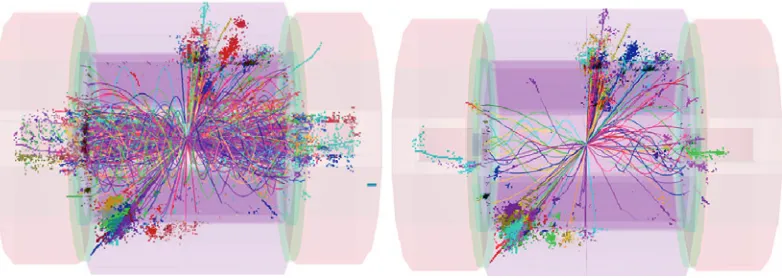
Figure 8.(left) Reconstructed particles in a simulated e+e−→H+H−→tbbt event at 3 TeV with background fromγγ→hadrons overlaid. (right) the effect of applying tight timing cuts on the reconstructed cluster times [2].

Theγγ→hadron events show a harder transverse momentum spectrum than the incoherent pairs. These events deposit a large amount of visible energy in the detector. During a bunch train 5000 tracks with a total momentum of 7 TeV, and a total energy of 19 TeV are deposited in the calorimeters. To avoid spoiling the precision measurements this background has to be identified and rejected.

3.2.1 Rejection of Background Particles

Due to the small bunch spacing the background from several bunch crossings will pile up over a physics event. To reject the background particles fromγγ→hadron events a time-stamping window of 10 ns (corresponding to 20 BX) is required in each sub-detector except for the barrel of the hadronic calorimeter, where a relaxed reconstruction window of 100 ns is possible. The single hit resolution in each sub-detector has to be about 1 ns [2].

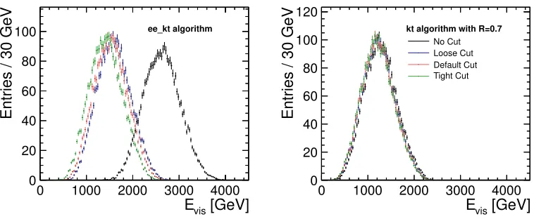
Figure 8 (left) shows a multi-jet event overlaid with theγγ → hadron background in the 10 ns reconstruction window of the detectors. The total background energy is 1.2 TeV. The rejection of the background particles is based on the average time of the cluster in the calorimeters, which can be precisely estimated from the many hits in an individual cluster. The timing cuts depend on particle type (charged/neutral), the transverse momentum, and the detector region [2]. Three different levels of timing cuts – loose, default and tight – were applied in the standard reconstruction for the con-ceptual design report. In Figure 8 (right) the tight timing cuts were used to reject the background. The remaining energy from the background particles is only 100 GeV, with negligible impact on the underlying hard interaction.

[GeV]

vis

E

0 1000 2000 3000 4000

Entries / 30 GeV

0 20 40 60 80

100 ee_kt algorithm

[GeV]

vis

E

0 1000 2000 3000 4000

Entries / 30 GeV

0 20 40 60 80 100 120

kt algorithm with R=0.7 No Cut Loose Cut Default Cut Tight Cut

Figure 9. Reconstructed jet energy distributions for different jet clustering algorithms and timing cuts. Left: DurhamkT-algorithm, Right:kT-algorithm including beam jets [2].

3.3 Detector Benchmark Studies and Physics at CLIC

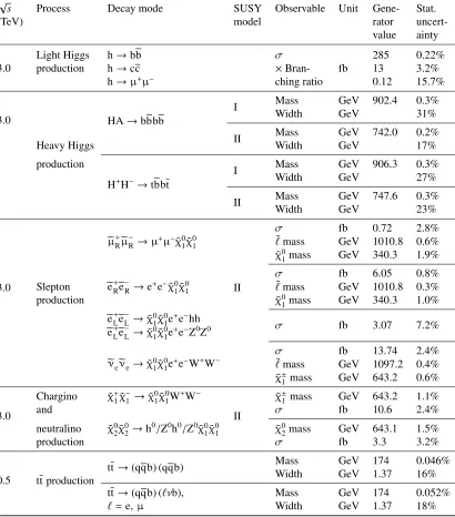
Detector benchmark studies were performed to evaluate the impact of the CLIC beam structure and background conditions on physics observables at √s=3 TeV. All detector benchmark studies were performed with full Geant4 simulation, overlaid withγγ → hadron backgrounds, and fully recon-structed. The sample sizes correspond to 2 ab−1 of integrated luminosity, or about four years of nominal operation. The generator values and the results for the benchmark studies described in the following are summarised in Table 2. The benchmark processes consist of rare Standard Model Higgs decays and typical signatures of new physics: missing energy, high momentum leptons, and multi-jet final states. The parameters of the Supersymmetry models (referred to as model I and II) used are described in [10].

3.3.1 Standard Model Higgs Measurements

A linear collider allows for the precise measurement of the fundamental properties of the Higgs boson. As the vector-boson fusion cross-section rises with the centre-of-mass energy, more Higgs bosons are produced at √s = 3 TeV, which gives access to rare decays, such as the Higgs decaying into two muons. Figure 10 (left) shows the different cross-sections for Higgs production, the rising vector-boson fusion process (Hνν) can be clearly seen.

Figure 10 (right) shows the invariant mass of the di-muon system after full simulation and re-construction. The peak for the Higgs decaying into muons is clearly visible above the background. To not smear out the signal peak an excellent momentum resolution is required. With 2 ab−1a sta-tistical uncertainty of 15.7% on the measurement of the cross-section times branching-ratio can be achieved [11, 12]. Due to the larger event rate the branching ratio for c- and b-quarks can be mea-sured with better precision (cf. Table 2).

3.3.2 Slepton Pair Production

neu-Table 2.Summary table of the CLIC benchmark analyses results. All studies at a centre-of-mass energy of 3 TeV are performed for an integrated luminosity of 2 ab−1_{. The study at 500 GeV assumes an integrated}

luminosity of 100 fb−1(Table abridged from CDR [2]).

√

s Process Decay mode SUSY Observable Unit Gene- Stat.

(TeV) model rator

uncert-value ainty

3.0

Light Higgs h→bb σ

fb

285 0.22%

production h→cc ×Bran- 13 3.2%

h→μ+μ− ching ratio 0.12 15.7%

3.0 HA→bbbb

I Mass GeV 902.4 0.3%

Width GeV 31%

II Mass GeV 742.0 0.2%

Heavy Higgs Width GeV 17%

production

H+H−→tbbt

I Mass GeV 906.3 0.3%

Width GeV 27%

II Mass GeV 747.6 0.3%

Width GeV 23%

3.0

μ+

Rμ−R→μ+μ−χ˜01χ˜01

II

σ fb 0.72 2.8%

˜

mass GeV 1010.8 0.6%

˜

χ0

1mass GeV 340.3 1.9%

e+_Re−_R→e+e−χ˜0 1χ˜01

σ fb 6.05 0.8%

Slepton ˜mass GeV 1010.8 0.3%

production χ˜0

1mass GeV 340.3 1.0%

e+_Le−_L→χ˜0 1χ˜

0

1e+e−hh σ _{fb 3.07 7.2%}

e+_Le−_L→χ˜0

1χ˜01e+e−Z 0_Z0

νeνe→χ˜01χ˜01e+e−W+W−

σ fb 13.74 2.4%

˜

mass GeV 1097.2 0.4%

˜

χ±

1 mass GeV 643.2 0.6%

3.0

Chargino χ˜+₁χ˜−₁ →χ˜0 1χ˜

0 1W+W−

II

˜

χ±

1 mass GeV 643.2 1.1%

and σ fb 10.6 2.4%

neutralino χ˜0 2χ˜02→h

0_/Z0_h0_/Z0_χ˜0

1χ˜01 χ˜02mass GeV 643.1 1.5%

production σ fb 3.3 3.2%

0.5 tt production

tt→(qqb) (qqb) Mass GeV 174 0.046%

Width GeV 1.37 16%

tt→(qqb) (νb), Mass GeV 174 0.052%

[GeV]

s

0 1000 2000 3000

HX) [fb]

→

-e

+

(e

σ

-2 10

-1 10

1 10 2 10

e

ν

e

ν

H

-e + H e

H Z

H H Z

H t t

e

ν

e

ν

H H

Di-muon invariant mass [GeV]

105 110 115 120 125 130 135

Events / 0.5 GeV

0 20 40 60 80

-μ

+

μ →

h

ν ν

-μ

+

μ

-e

+

e

-μ

+

μ

Figure 10.Left: Higgs production cross-section formh =120 GeV. Right: Di-muon invariant mass spectrum, the peak at the Higgs mass is clearly visible above the background [2].

tralino mass can be extracted from the endpoints of the lepton energy spectrum [5]. Figure 11 shows the distribution of the reconstructed energy of muons after background subtraction. The shape differs from the expected rectangular one because of the luminosity spectrum and finite momentum resolu-tion. The figure also contains a fit which takes into account these imperfections. The pair production of scalar electrons and scalar neutrinos was also studied. The masses of these sleptons and the neu-tralino can be measured with a statistical uncertainty of a few GeV (cf. Table 2).

3.3.3 Gaugino Pair Production

The final state of the different chargino and neutralino pair production processes is always four jets (from different boson pairs) and missing energy (in the neutralinoχ0₁):

e+e−→χ+₁χ−₁ →χ0₁χ0₁W+W−

e+e−→χ0₂χ0₂→χ0₁χ0₁hh

e+e−→χ0₂χ₂0→χ0₁χ0₁Zh.

To separate the different processes – and measure the mass of the respective gaugino – the jet masses have to be reconstructed, so that the original bosons can be identified. Figure 12 shows the recon-structed di-jet mass for the three different Gaugino pair production processes; the peak of each process is well separated from the others. This demonstrates that the particle flow reconstruction of boosted bosons performs well in the CLIC environment [13].

3.3.4 Heavy Higgs Bosons

E [GeV]

Events

Fit:S+B(Data)-B(MC), events: 2845 5.57

±

= 1014.29

μ∼

M

/ ndf 24.5 /45

2

χ

6.38 ,

±

= 341.75

0

χ∼

M

Figure 11. Reconstructed muon energy spectrum for the smuon pair production process after back-ground subtraction.

[GeV]

jj,1

M

40 60 80 100 120 140 160

[GeV]

M

Figure 12. Scatter plot showing the reconstructed di-jet invariant masses of W, Z and h candidates in simulated e+e− →χ˜+₁χ˜−₁ and e+e−→ χ˜0

2χ˜ 0 2 signal events includingγγ →hadrons background. The peaks corresponding to the individual chargino and neutralino decays are indicated. The event samples were scaled to have a similar number of events for each channel [2].

]

Di-Jet Invariant Mass [GeV

600 800 1000 1200 1400

-1

Entries / 2 ab

0 20 40 60 80 100 120 HA -H + H WW ZZ tt+4b WWZ+ZZZ

]

Di-Jet Invariant Mass [GeV

600 800 1000 1200 1400

-1

Entries / 2 ab

0 50 100 150 -H + H HA WW ZZ tt+4b WWZ+ZZZ

Entries / 2 GeV 500 1000 1500

Top Mass [GeV]

100 150 200 250

Residuals

Normalize

d

-2 0 2

Entries / 2 GeV

200 400 600 800 1000 1200

Top Mass [GeV]

100 150 200 250

Residuals

Normalize

d

-2 0 2

Figure 14.Mass distribution for 6-jet events (left) and 4-jet events (right). Points with error bars show simulated data classified as signal events. The green histogram illustrates the contribution of non-tt background to the distribution. The blue line shows the fit of the top mass distribution [2].

3.3.5 ttat 500 GeV

The study of the top-quark would be a core part of a first CLIC stage [3]. The top-pair production was simulated at a centre-of-mass energy of 500 GeV and studied with a data sample corresponding to an integrated luminosity of 100 fb−1. Figure 14 shows the distributions of the reconstructed top-masses for the fully hadronic channel (both W-bosons decaying to four jets, and the semi-leptonic channel (one W-boson decaying to lepton and neutrino). In the fully hadronic channel a statistical uncertainty of about 80 MeV on the mass of the top-quark can be reached [14].

3.3.6 Summary

Precision measurements for a wide variety of new physics signatures can be performed at CLIC, despite the challenging background and beam conditions at 3 TeV. Rare Higgs decays profit from the larger cross-section at higher centre-of-mass energies. CLIC can also be used as a discovery machine complementary to the LHC. Table 3 lists the physics reach for hadron and electron–positron colliders with different centre-of-mass energies and integrated luminosities. A high energy electron–positron collider has advantages when precision measurements are required to find new physics. Due to the cleaner conditions electro-weak particles can be discovered in the full energy range of the collider up to a mass ofmx =

√

s/2. CLIC can also be sensitive to new physics far beyond its direct energy reach, for example, evidence for a Zwith Standard Model couplings could be found up to a Zmass of 20 TeV.

3.4 Physics and Detectors: Future Plans

Table 3.Physics reach for different colliders. TGC is short for Triple Gauge Coupling, and “μcontact scale” is short for LLμcontact interaction scaleΛwithg=1 [2, 15].

LHC14 SLHC14 LC800 CLIC3

100 fb−1 1 ab−1 500 fb−1 1 ab−1

squarks [TeV] 2.5 3 0.4 1.5

sleptons [TeV] 0.3 0.4 1.5

Z(SM couplings)[TeV] 5 7 8 20

2 extra dimsMD[TeV] 9 12 5–8.5 20–30

μcontact scale [TeV] 15 20 60

Higgs composite scale [TeV] 5–7 9–12 45 60

TGC (95%)(λγcoupling) 0.001 0.0006 0.0004 0.0001

There are many technological challenges for the sub-detectors, which require R&D. The vertex detector has to be ultra-thin, small-pixeled and fast. The main tracking detectors need an integrated design. The electronics for the sensors require fast-timing, while offering a low power-consumption and the ability for power-pulsing. The highly granular calorimeters require compact active layers and 1 ns hit time resolution. At the same time the engineering challenges for the support, stability, alignment, and cooling have to be met. These topics are part of an ongoing R&D effort for the post-CDR project phase of 2012–2016 [2].

4 Summary

The conceptual design reports for the Compact Linear Collider show good results, proving the fea-sibility of the accelerator and detector technologies. The drive-beam generation, and its deceleration in power extraction structures have been shown in CTF3. The RF power provided by the drive beam was used to accelerate a second beam with a gradient of 106 MV/m. The break-down rate of the accelerator cavities and PETS was reduced to the required level. Despite the challenging background conditions at CLIC precision physics measurements can be performed. Rare Higgs decays can be studied and extensions of the Standard Model can be explored with great precision. CLIC therefore offers a promising possibility to study fundamental physics complementary to the LHC.

References

[1] M. Aicheler, P. Burrows, M. Draper, T. Garvey, P. Lebrun, K. Peach, N. Phinney, H. Schmickler, D. Schulte, N. Toge, eds.,A Multi-TeV Linear Collider based on CLIC Technology: CLIC Con-ceptual Design Report(CERN, 2012), JAI-2012-001, KEK Report 2012-1, PSI-12-01, SLAC-R-985

[2] L. Linssen, A. Miyamoto, M. Stanitzki, H. Weerts, eds.,Physics and Detectors at CLIC: CLIC Conceptual Design Report(CERN, 2012), ANL-HEP-TR-01, CERN-20003, DESY 12-008, KEK Report 2011-7

[3] P. Lebrun, L. Linssen, A. Lucaci-Timoce, D. Schulte, F. Simon, S. Stapnes, N. Toge, H. Weerts, J.D. Wells, eds.,The CLIC Programme: towards a staged e+e−Linear Collider exploring the Terascale(CERN, 2012), ANL-HEP-TR-12-51, KEK Report 2012-2, MPP-2012-115

[5] M. Battaglia, J.J. Blaising, J. Marshall, J. Nardulli, M.A. Thomson, E. van der Kraaij,Physics performances for scalar electrons, scalar muons and scalar neutrinos searches at CLIC, CERN-LCD-Note-2011-018 (2011)

[6] A. Münnich, A. Sailer,The CLIC_ILD_CDR Geometry for the CDR Monte Carlo Mass Produc-tion, CERN-LCD-Note-2011-002 (2011)

[7] C. Grefe, A. Münnich,The CLIC_SiD_CDR Geometry for the CDR Monte Carlo Mass Produc-tion, CERN-LCD-Note-2011-009 (2011)

[8] P. Chen, An Introduction to Beamstrahlung and Disruption, inFrontiers of Particle Beams, edited by M. Month, S. Turner (1988), Vol. 296 ofLecture Notes in Physics, Berlin Springer Verlag, pp. 495–532

[9] P. Chen, V. Telnov, Phys. Rev. Lett.63, 1796 (1989)

[10] M.A. Thomson, M. Battaglia, J. Ellis, G. Giudice, A. Lucaci-Timoce, F. Teubert, J. Wells, J.J. Blaising, S. Martin,The physics benchmark processes for the detector performance studies of the CLIC CDR, CERN-LCD-Note-2011-016 (2011)

[11] C. Grefe, Light Higgs decay into muons in the CLIC_SiD CDR detector, CERN-LCD-Note-2011-035 (2011)

[12] C. Grefe, T. Lastovicka, J. Strube, accepted by Eur. Phys. J. C (2012),hep-ex/1208.2890 [13] T. Barklow, A. Münnich, P. Roloff,Measurement of chargino and neutralino pair production at

CLIC, CERN-LCD-Note-2011-037 (2011)

[14] K. Seidel, S. Poss, F. Simon,Top quark pair production at a 500 GeV CLIC collider, CERN-LCD-Note-2011-026 (2011)