Cross-Layer Approaches for Architectural Vulnerability Estimation to Improve the Reliability of Superscalar Microprocessors

ABSTRACT

WIBOWO, BAGUS PRASETYO. Cross-Layer Approaches for Architectural Vulnerability Estimation to Improve the Reliability of Superscalar Microprocessors . (Under the direction of James Tuck.)

Processor soft error rates are projected to increase as feature sizes scale down necessitating the adoption of reliability enhancing schemes, but power and performance overhead remain a concern of such techniques. Dynamic cross-layer techniques are a promising way to improve the cost effectiveness of resilient systems. As a foundation for making such a system, we propose AVF-CL, an online cross-layer approach for estimating the architectural vulnerability of a processor core that works by combining information from software, compiler, and microar-chitectural layers at runtime. The hardware layer combines the metadata from software and compiler layers with microarchitectural measurements to estimate architectural vulnerability online.

We describe our design and evaluate it in detail on a set of SPEC CPU 2006 applications. We find that our online Architectural Vulnerability Factor (AVF) estimate is highly accurate with respect to a postmortem AVF analysis, with only 0.46% average absolute error. Also, our AVF-CL design incurs negligible performance impact for SPEC2006 applications and about 1.2% for a Monte Carlo application, requires approximately 1.4% area overhead, and costs about 3.3% more power, on average. We compare our technique against two prior online AVF estimation techniques, and our evaluation finds that our approach, on average, is more accurate. Our case study of a Monte Carlo simulation shows that our AVF estimate can take into account the inherent resiliency of the algorithm. Finally, we demonstrate the effectiveness of our approach using a dynamic protection scheme that limits vulnerability to soft errors while reducing the energy consumption by 4.8%, on average and with a target normalized Soft Error Rate (SER) of 10%, compared to enabling a simple parity+ECC protection at all times. When paired with a more sophisticated protection scheme, our approach can achieve even more significant energy overhead reduction by as much as 94.2%, on average, for triple modular redundancy (TMR) technique.

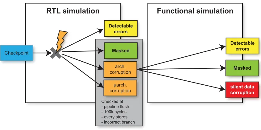
To gain insight, we investigate further the AVF of all major in-core memory structures of an out-of-order superscalar processor. In particular, we focus on the vulnerability factors for detectable and unrecoverable errors (DUEAVF) and silent data corruptions (SDCAVF) across windows of execution to study their characteristics, time-varying behavior, and their pre-dictability using a linear regression trained offline. To determine DUEAVF and SDCAVF, we perform a fault injection campaign over a window of execution. We inject faults on a detailed microarchitectural simulation (using RTL simulation) but run-to-completion on a much faster functional simulation. The results are compared with a clean run with no injected faults to identify and classify errors. More than 35 million microarchitectural level fault injection simulations are conducted to collect our data.

Our study shows that, similar to AVF, DUEAVF and SDCAVF vary over time and across applications. We also find significant differences in DUEAVFand SDCAVF across the processor structures we studied. Furthermore, we find that DUEAVF can be predicted using a linear regression with similar accuracy as AVF estimation. However, SDCAVF could not be predicted with the same level of accuracy.

© Copyright 2017 by Bagus Prasetyo Wibowo

Cross-Layer Approaches for Architectural Vulnerability Estimation to Improve the Reliability of Superscalar Microprocessors

by

Bagus Prasetyo Wibowo

A dissertation submitted to the Graduate Faculty of North Carolina State University

in partial fulfillment of the requirements for the Degree of

Doctor of Philosophy

Computer Engineering

Raleigh, North Carolina

2017

APPROVED BY:

Gregory Byrd Eric Rotenberg

Xiaohui Gu James Tuck

DEDICATION

Untuk mama Menuk Retnaningsih dan papa Wulan Adi Susetyo. Untuk istriku, Rasi.

Untuk kedua malaikat kecilku, Fathina dan Salma.

––––––––––

To my mom, Menuk Retnaningsih, and my dad, Wulan Adi Susetyo. To my wife, Rasi.

BIOGRAPHY

ACKNOWLEDGMENTS

It would be impossible for me to complete this work without the help of many people. First of all, I would like to thank my advisor, Dr. James Tuck, for his constant support, counsel, and advice during my Ph.D. studies. His dedication inspires me to keep working, and it is a great honor for me to work with him.

I would also like to express my appreciation to my committee Dr. Gregory Byrd, Dr. Eric Rotenberg, Dr. Xiaohui (Helen) Gu, and Dr. Daowen Zhang for their dedication in their service on my committee. I also thank them for their valuable feedback and advice for this thesis.

Many thanks are due to Abhinav Agrawal and Thomas Stanton for collaborating work on cross-layer fault tolerance project, and also to my colleagues in Dr. Tuck’s group Joonmoo Huh, Tiancong Wang, David Mabe, Alexander Simpson, Laxman Sole, as well as other CESR colleagues Amro Awad, Yipeng Wang, Seunghee Shin, Abdullah Mughrabi, Rangeen, Hussein Elnawawy, Vinesh Srinivasan, Mohammad Alshboul, and Satish Tirukkovalluri. Numerous thanks to Elliott, Brandon, and Niket for their help in solving some issues while adapting FabScalar infrastructure. I also thank Randy Widialaksono for helping me running millions of fault injection simulations, and also Sigit Pambudi for all the small chats in the midst of our busy work.

Now, I must thank my wife, Rasi Fitria, for her inestimable support and time that, without her help, it would take me many more years before I could complete my Ph.D. studies. My life would not be so colorful without the presence of her and my two little daughters, Fathina and Salma. I truly thank them for sharing their unlimited fuel of happiness while I’m striving with my Ph.D. studies. Finally, I sincerely thank my parents for their continuous support and prayer. I wish my accomplishment, which is also part of their accomplishment, could make them proud.

TABLE OF CONTENTS

LIST OF TABLES . . . viii

LIST OF FIGURES . . . ix

Chapter 1 INTRODUCTION . . . 1

1.1 Improving Reliability by Estimating System Vulnerability . . . 2

1.2 System Vulnerability for Specific Types of Failure . . . 4

1.3 Using Cross-Layer Information to Improve Silent Data Corruption Predictability 5 1.4 Contributions . . . 6

1.5 Organization of This Thesis . . . 7

Chapter 2 BACKGROUND . . . 8

2.1 Soft Errors . . . 8

2.1.1 The Projected Trend of Soft Error Rate . . . 9

2.1.2 Techniques to Mitigate Soft Errors in Computer Systems . . . 10

2.1.3 Soft Errors Manifestation . . . 10

2.2 Measuring Reliability of a System . . . 11

2.2.1 Architectural Vulnerability Factor . . . 11

2.2.2 Estimating Architectural Vulnerability Factor . . . 11

2.2.3 Online Estimation of Architectural Vulnerability Factor . . . 16

2.3 Canonical Superscalar Processors . . . 18

Chapter 3 AVF-CL: AN ACCURATE CROSS-LAYER APPROACH FOR ONLINE ARCHITECTURAL VULNERABILITY ESTIMATION . . . 21

3.1 Introduction . . . 21

3.2 Cross-Layer Vulnerability Estimation . . . 22

3.2.1 Cross-Layer Metadata . . . 22

3.2.2 Cross-Layer Predictor . . . 24

3.2.3 Accuracy with Low Overhead . . . 25

3.3 Basic AVF-CL Design . . . 26

3.3.1 Reliability Calculation Logic . . . 27

3.3.2 Compiler Support for Metadata . . . 32

3.3.3 The Pipeline . . . 33

3.3.4 Timestamp and Vbit Accumulation width . . . 34

3.3.5 Sampled reliability estimation . . . 34

3.4 Optimized AVF-CL Design . . . 35

3.4.1 Vulnerability Calculation Logic . . . 35

3.4.2 Compiler Support for Metadata . . . 41

3.4.3 Time-stamp, Duration, and Vbit Accumulation width . . . 44

3.5 Miscellaneous Issues . . . 44

3.5.1 Handling context switching . . . 44

3.5.2 Other Registers and Logic . . . 45

3.6 Evaluation for Basic AVF-CL Design . . . 45

3.6.1 Methodology . . . 45

3.6.2 Reliability Estimation and Accuracy . . . 47

3.6.3 Reducing Power and Performance Overhead by Sampling . . . 52

3.7 Evaluation for Optimized AVF-CL Design . . . 52

3.7.1 Methodology . . . 52

3.7.2 Reliability Estimation and Accuracy . . . 56

3.7.3 AVF-CL Overhead . . . 56

3.8 Case Study 1: Monte Carlo Simulation . . . 60

3.8.1 Results . . . 62

3.9 Case Study 2: Dynamic Protection using AVF-CL . . . 63

3.9.1 Soft Error Rate Results . . . 65

3.9.2 Power Overhead Results . . . 67

3.9.3 Dynamic Protection using AVF-CL Summary . . . 68

3.10 Summary . . . 68

Chapter 4 CHARACTERIZING THE IMPACT OF SOFT ERRORS ACROSS MI-CROARCHITECTURAL STRUCTURES AND IMPLICATIONS FOR PRE-DICTABILITY . . . 70

4.1 Introduction . . . 70

4.2 Fault Injection Simulation . . . 71

4.2.1 Hardware Fault Model . . . 72

4.2.2 Detailed RTL with fault injection simulations . . . 72

4.2.3 High-level functional simulations . . . 74

4.2.4 Categorizing fault injection outcomes . . . 75

4.3 Experimental Methodology . . . 75

4.4 Evaluation . . . 77

4.4.1 AVF, SDCAVF, and DUEAVF comparison . . . 77

4.4.2 Correlation of SDCAVF and DUEAVFwith AVF . . . 79

4.4.3 SDCAVF and DUEAVF Per Structures . . . 79

4.5 Estimating SDCAVF and DUEAVF using regression analysis . . . 81

4.5.1 Results . . . 81

4.6 Program Sections with High SDCAVF Discussion . . . 85

4.6.1 High SDC Rate Program Section forbitcount . . . 85

4.6.2 High SDC Rate Program Section forastar . . . 86

4.7 Summary . . . 86

Chapter 5 CROSS-LAYER APPROACHES FOR ESTIMATING SILENT DATA COR-RUPTION ARCHITECTURAL VULNERABILITY . . . 87

5.1 Software-Level Reliability Information for a Cross-Layer SDCAVF Estimation . 88 5.1.1 Software-Level Fault Models . . . 88

5.1.2 Limiting Software-Level Reliability Information Availability . . . 89

5.2 Evaluation . . . 90

5.2.3 The Impact of Limiting Software-Level Reliability Information Availability 94

5.3 Using Cross-Layer Information for Online SDCAVF Estimation . . . 96

5.3.1 Obtaining and Encoding SDCPVSat Compile Time . . . 99

5.3.2 SDCAVF Predictor Logic . . . 100

5.3.3 Compiler Support for Online SDCAVF Estimation . . . 103

5.3.4 Miscellaneous Issues . . . 104

5.3.5 Experimental Methodology . . . 104

5.3.6 Results . . . 105

5.4 Summary . . . 107

Chapter 6 RELATED WORK . . . 108

Chapter 7 CONCLUSION . . . 113

BIBLIOGRAPHY . . . 115

APPENDICES . . . 123

Appendix A LIST OF MICROARCHITECTURAL VARIABLES USED FOR LIN-EAR REGRESSION BASED AVF ESTIMATION . . . 124

A.1 Microarchitectural Variables Collected in Brutus C++ Microarchitectural Timing Simulator . . . 124

A.2 Microarchitectural Variables Collected in FabScalar RTL Simulation . . . 135

LIST OF TABLES

Table 3.1 Vulnerable bits per structure and opcode for the basic AVF-CL design. . 30

Table 3.2 Vulnerable bits per structure and opcode for the optimized AVF-CL design. 40 Table 3.3 Simulator configuration for basic AVF-CL design evaluation . . . 46

Table 3.4 Basic AVF-CL design configurations . . . 46

Table 3.5 Simulator configuration for optimized AVF-CL design evaluation . . . . 53

Table 4.1 Simulator configuration for soft errors characterization study . . . 75

Table 4.2 Midpoint ( ˜p) and confidence interval for 64,000 trials and X successes, calculated using Equation 2.5 . . . 77

Table 4.3 Pearson correlation coefficient (R) between AVF with DUEAVF and AVF with SDCAVF . . . 79

Table 4.4 DUEAVF per structure . . . 80

Table 4.5 SDCAVFper structure . . . 80

Table 4.6 Instruction mix for each benchmark. . . 81

Table 5.1 The minimum number of basic blocks to achieve certain dynamic instruc-tion coverage of the representative SimPoint region. . . 91

Table 5.2 Regression-based SDCAVF Estimation Model using SDCPVF-OP trained using "leave-one-out" strategy . . . 93

LIST OF FIGURES

Figure 2.1 Raw soft error rate per chip is expected to increase as we continue progressing the transistor technology to smaller feature size and pack

more transistors per chip [Ibe10; DW11]. . . 9

Figure 2.2 System vulnerability layers. . . 15

Figure 2.3 System SDC vulnerability layers. . . 17

Figure 2.4 An example of a canonical superscalar processor. . . 19

Figure 3.1 Determining vbits. . . 24

Figure 3.2 Overall idea of AVF-CL. . . 24

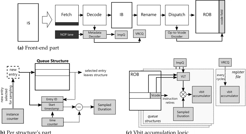
Figure 3.3 Simplified superscalar processor pipeline design with dark shaded blocks indicating our modifications (components not drawn to scale). . . 27

Figure 3.4 Details of Vbit calculation for the issue queue. . . 28

Figure 3.5 Micro-architecture modifications to support AVF-CL. . . 35

Figure 3.6 Compiler flow for generating metadata. . . 41

Figure 3.7 Instantaneous vulnerability estimation comparison on one simpoint of two applications. . . 48

Figure 3.8 Mean absolute error comparison of combined SRAM structures. . . 48

Figure 3.9 Accuracy comparison across several structures for one simpoint of 458.sjeng. . . 50

Figure 3.10 Area and energy overhead of AVF-CL. . . 51

Figure 3.11 Mean absolute error, performance, and energy overhead of AVF-CL.S.ic. 53 Figure 3.12 Mean absolute error of estimating AVF on all structures we monitor. . . 57

Figure 3.13 Performance comparison of enabling AVF-CL with and without NOP-lane. 57 Figure 3.14 Performance overhead for Monte Carlo. . . 58

Figure 3.15 Area and power overhead of AVF-CL. . . 60

Figure 3.16 Calculatingπusing Monte Carlo Simulation[Ros] . . . 61

Figure 3.17 Vulnerability factor comparison over time for Monte Carlo application. 62 Figure 3.18 Vulnerability Factor Comparison for Monte Carlo application. The VF-reduction shows how much VF reduced due to algorithm level derating. The values shown on top of each bar are the magnitude of VF-reduction. 63 Figure 3.19 Timing illustration of dynamic protection using AVF-CL+window ap-proach. . . 64

Figure 3.20 Timing illustration of dynamic protection using AVF-R+hist approach. 65 Figure 3.21 Impact of dynamic protection using AVF-CL+window on SER over time. 65 Figure 3.22 Impact of dynamic protection with various threshold on overall SER. . 66

Figure 3.23 Overall power overhead of dynamic protection using AVF-CL+window compared to static protection. . . 67

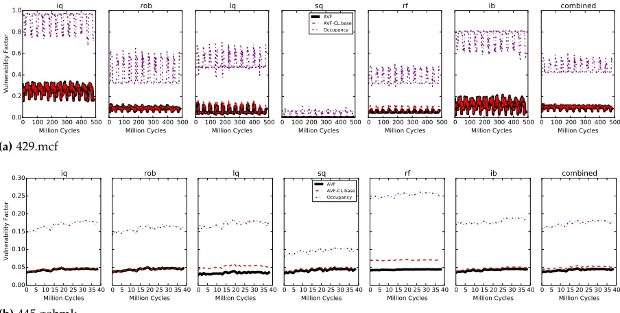
Figure 4.1 Overview of fault injection campaign at RTL simulation and, if needed, at functional simulation. . . 72 Figure 4.2 AVF, SDCAVF, and DUEAVFover the phases of execution (a). The zoomed

SDCAVF plots for bzip2, gcc, gobmk, astar, and dijkstra are shown in (b). These figures show the variation of both DUEAVF and SDCAVF across workloads as well as across the phases of execution. The red shaded area indicates statistical error bound with 95% confidence interval. . . 78 Figure 4.3 Overall DUEAVF, SDCAVF, and AVF and their estimation using regression

models, labeled asDUEAVF-reg,SDCAVF-reg, andAVF-reg, respectively. . 82 Figure 4.4 Overall AVF, SDCAVF, and DUEAVF estimation accuracy comparison

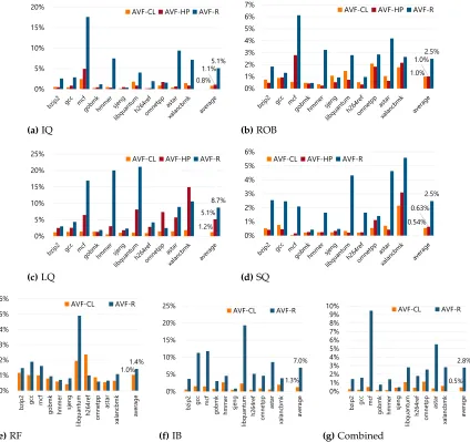
using two different metrics: (a) mean absolute error, and (b) mean ratio error. Using mean ratio error is more meaningful for this comparison as it normalizes the relative error to the actual value. . . 83 Figure 4.5 AVF, SDCAVF, and DUEAVFestimation MRE per structure averaged across

all workloads. . . 84 Figure 4.6 Architectural state corruption vulnerability factor compared against

SDCAVF (a), and architectural state corruption vulnerability factor to SDCAVF derating factor (b). . . 84

Figure 5.1 Accuracy comparison of estimating SDCAVF using software-level reliabil-ity information. . . 92 Figure 5.2 The impact of picking various N basic blocks as representatives for

obtaining SDCPVF. . . 95 Figure 5.3 MRE comparison of building an SDCAVF estimate model using

cluster-based basic block selection normalized to the ones that use frequency-based basic block selection. . . 96 Figure 5.4 Comparison of SDCAVF estimation using fault injection and cross-layer

regression model over execution windows. . . 97 Figure 5.5 Overall flow of building and using online SDCAVFestimator. . . 98 Figure 5.6 Encoding and passing SDCPVSto hardware through SDCPVSLUT. . . 101 Figure 5.7 Additional hardware (a) at decode stage for early SDCPVS averaging and

(b) at decode and commit stages for late SDCPVS averaging. . . 101 Figure 5.8 SDCAVF calculation logic. . . 103 Figure 5.9 Accuracy comparison of estimating SDCAVFusing offline approach and

two SDC-CL configurations. The plots show the accuracy in two different metrics: (a) mean absolute error, and (b) mean ratio error. . . 106 Figure 5.10 MRE comparison of SDC-CL online with various availability of SDCPVS

Chapter

1

INTRODUCTION

In recent decades, advances in computer system design technology have been driven by two main factors: performance and power consumption. Significant efforts have been made to opti-mize the trade-off between performance and power consumption across all areas of computer system research such as algorithm, compiler, operating system, microarchitecture, and chip fabrication technology. In addition to these two factors, another important concern, especially in the case of large-scale systems such as data centers or high performance computing systems, is system reliability.

Although system reliability concerns have typically been confined to large-scale systems, they may increasingly apply to other systems as well. There has been a growing concern about the reliability of current and future systems, including commodity computer systems, as microprocessors’ minimum feature sizes continue to scale down and the number of transistors per chip continues to increase. Prior literature has projected that the combination of these two factors increases the susceptibility of hardware to soft errors [Bor05; Con07; Li07; Ibe10; DW11]. For systems with stringent reliability requirements, this decline in reliability must be dealt with in some way. There are many well known strategies for improving fault tolerance, like redundancy [Rot99; Muk02; Ten02; Oh02; Rei05b; Rei05c; Sha06; Shy09; Zha10] and Error-Correcting Codes (ECC) [PW72]. These approaches provide some improvement in reliability, with varying expenses in terms of hardware, performance, and power overhead.

is needed when running a critical application, when running an essential part of a program, or when approaching the end of their expected lifetime. Thus, rather than over-provisioning reli-ability, a better approach would be to use a judicious and flexible technique that provides just enough reliability to ensure a better trade-off between power, performance, and reliability. The additional cost of such techniques can be justified by the cost savings from avoiding protection when it is not needed. Such approach is known as a dynamic reliability enhancement [Wal07; Bis09; Sou07; Wib16].

A prerequisite for such a dynamic system, wherein online reliability trade-offs are possible, would be a cheap and effective reliability measurement technique. Ideally, such a measurement technique would be cross-layer and account for both hardware and software resiliency. While cross-layer approaches could be used to describe the interaction of many different layers, this work focuses specifically on the software and microarchitectural layers. Furthermore, our work also focuses on the reliability estimation schemes, with regard to soft errors, for superscalar microprocessor systems.

1.1

Improving Reliability by Estimating System Vulnerability

Prior work has investigated online estimation for reliability of a microprocessor, usually in the form of predicting the Architectural Vulnerability Factor (AVF) [Li08c; Fu06; Wal07; Bis09; Dua09; Sou07; SK10]. However, many of these approaches take a processor-centric view and are unable to fully account for cross-layer effects. For example, [Li08c] use a fault injection strategy, but it is only practical for it to propagate faults as far as branches and stores. This means it is unable to derate some forms of benign errors, including ones that are corrected by software. Some other approaches [Fu06; Wal07; Bis09; Dua09] use hardware performance counters to estimate AVF at runtime. Even though the model is built based on post-mortem AVF, which is cross-layer in principle, the hardware performance variables themselves are not sensitive to changes in software layer reliability. The same sequence of code used in different algorithms might have different reliabilities, but a predictor that is based solely on the value of performance counters cannot recognize such a difference. Another approach [Sou07] estimates AVF of a processor’s Reorder Buffer (ROB) by simply tracking its occupancy. However, since speculative instructions are also tracked, this gives high upper-bound estimates.

the vulnerability of software to soft errors. It is determined through careful calibration using profile data collected from a prior run of the program. However, such calibration may not always be accurate since it is sensitive to input. Also, the article does not describe how to support all structures in the core, the register file in particular.

In this work, we propose AVF-CL, a combined hardware and software technique that is capable of measuring the cross-layer reliability of a core in combination with its software stack at run time. Our approach is based on the concept of Architecturally Correct Execution (ACE) analysis [Muk03], but we develop a way of doing such analysis at runtime, instead of post-mortem. To determine ACE information, which is usually obtained post-mortem, our approach uses any available cross-layer information at runtime. In hardware, we add inexpensive logic that estimates and accumulates the number of bits per instruction and per structure that may be needed for Architecturally Correct Execution (such bits are called ACE bits). Along with this hardware, information about the software is passed to the hardware in the form of metadata. While the program executes, the metadata is used by the predictor to further exclude some bits from being estimated as ACE. All instructions that ultimately retire add their estimated ACE bits into a cumulative count for the entire core. This cumulative measure of vulnerability is exposed to software and can be used for online reliability adaptation, and it can also be used to estimate AVF or other reliability metrics.

Our design is able to achieve high accuracy and low overhead. It achieves high accuracy through a combination of two key approaches. First, the logic we add to the core carefully tracks ACE bits on a per instruction and per structure basis. This allows us to accurately exclude bits from structures that do not matter on a per opcode basis. Second, the metadata allows us to accurately derate the register file and some instructions that do not matter. The design achieves low overhead by limiting the amount of logic added to each processor structure and by limiting the resources devoted to metadata. In particular, to count the number ACE bits for an instruction in a specific processor structure, we need to know the number of ACE bits it used in that structure and how long it was active in that structure. Rather than track duration for each instruction, we sample the duration of instructions periodically. Such samples are used as an approximation of all instructions that commit during an interval of time. Later in this thesis, we describe how best to make this approximation for each structure in the processor. To deal with metadata, we require that it be encoded in the unused bits of instructions, similar to Argus [Mei07]. Such an approach requires additional logic to decode metadata and forward it to relevant stages later in the pipeline, but we show that this overhead is modest.

bits in the key processor structures are not ACE. We have identified two main purposes of metadata: (a) to identify an instruction whose results are not ACE, and (b) to identify registers that are not ACE. The compiler can easily generate case (b) using a form of vulnerable register analysis (discussed in Section 3.4.2.2), and often the programmer can identify case (a) (discussed in Section 3.8). Both of these features are easy to integrate into a compiler toolchain and do not rely on derating factors, which are non-intuitive for programmers working at a source level. While more work is needed to show the full advantage of this approach, it may facilitate the development of programmer and compiler-driven reliability optimization.

Our proposed AVF-CL design relies on metadata to capture program level resiliency, with regard to soft errors, based on the information obtained from compiler analyses and programmer markings. Programmer’s involvement in enhancing metadata is particularly important to identify algorithm level resiliency in the program. Otherwise, the compiler would require some more expensive technique (such as fault injection) to identify such resiliency.

1.2

System Vulnerability for Specific Types of Failure

The severity of soft errors to the system depends on when and where a soft error happens. Some soft errors could be masked and hidden by the operation of the hardware or software and cause zero impact on the correctness of program execution. Others could manifest as detectable error, which could be recoverable (DRE) or unrecoverable (DUE), or Silent Data Corruption (SDC). Since SDCs do not produce obvious failures, there is significant interest and need in finding inexpensive ways to prevent them. Our work continues further by investigating the impact of soft errors on the system behavior.

Rather than protecting a system continuously from SDCs, it may be possible to sporadically protect when SDCs are more likely to occur. While predicting AVF has been the subject of much prior work [Fu06; Wal07; Bis09; Li08c; Dua09; SK10; Wib16], predicting SDC has not. In fact, few studies have deeply characterized SDC rates. Most prior work looks at software-level SDC rate analysis [Har12b; Har12a; LT13; Har14; Lu14]. They observe the inter-workload variation of the SDC rate. However, it remains unclear how the software-level SDC rate relates to the system-level SDC rate. Furthermore, the variation of SDC rate across the execution of a program is currently not well understood. Understanding the change of SDC rate is critical for building an efficient dynamic reliability enhancement that mitigates SDC at runtime.

of a modern superscalar processor. To determine DUEAVF and SDCAVF, we perform a fault injection campaign over a window of execution. We inject faults on a detailed microarchitec-tural simulation (using RTL simulation) but run-to-completion on a much faster functional simulation if necessary. Each fault injection run is compared against a clean run with no injected faults to identify it as masked, DUE, or SDC.

Next, we use the time-varying DUEAVF and SDCAVF to train an offline linear regression model for predicting AVF, DUEAVF, and SDCAVF. Prior work has demonstrated that AVF can be predicted with reasonable accuracy [Wal07; Bis09]. We confirm that result and also demonstrate that DUEAVFcan be predicted with similar accuracy. However, the SDCAVFcannot be predicted with similar accuracy. This suggests that silent data corruption manifests differently from both AVF and DUEAVF and that predictors that intend to predict SDCAVF may need a different approach or additional information not available to our model.

1.3

Using Cross-Layer Information to Improve Silent Data

Corrup-tion Predictability

We further investigate how the accuracy of SDCAVF estimation model could be improved. We identify a hint that software-level reliability information could be the key that explains the variation of SDCAVF over the phases of execution and across workloads. We study further and evaluate the use of software-level information on a linear regression model for estimating SDCAVF and find that the accuracy improves by 5.19×, on average, to a level similar to that of DUEAVF and AVF predictors.

Furthermore, because our software-level information is derived from fault injection ex-periments which are not as simple as a variable look up in simulator, we wish to reduce the cost associated with collecting that data. Therefore, we also evaluate two approaches to reduce the amount of software-level reliability information required and study the impact on SDCAVF accuracy. Our evaluation shows that using either approach doesn’t impact the accuracy significantly, on average. When we limit the availability of software-layer reliability information to only three basic blocks (21×cost reduction, on average), it only increases the error from 56.4% to 71.8% (a 27.3% increase), on average.

evaluate the performance of our proposed design on estimating SDCAVF online and find that on average it achieves a similar level of accuracy compared to the offline approach with only an increase in MRE by 17%.

1.4

Contributions

In summary, the work presented in this thesis makes the following contributions, grouped into three categories. The first category is related to the design of cross-layer approach for estimating architectural vulnerability online. In this category, we describe the design of a cross-layer technique for estimating the combined vulnerability of software and hardware. The proposed metadata is easy to compute with standard compiler tool flows, and it is accurate when compared to a conventional postmortem AVF analysis. Next, we thoroughly evaluate our design using the SPEC CPU 2006 applications. Then, we demonstrate the effectiveness of our cross-layer design on a case study of a resilient Monte Carlo algorithm. Finally, we use our monitor to limit the vulnerability of the core within a soft error rate target by dynamically enabling and disabling simple parity+ECC protection on all major in-core memory structures and show that even with the cost of monitoring included, it yields significant power savings compared with using protection all of the time. We also show that even with a very tight error rate target, our approach can still find an opportunity to save power consumption.

For the second category, we study the impact of soft errors on the system behaviors and their implications for predictability. In this study, we first explain how we do fault injection using detailed microarchitectural simulations and subsequently transferred to functional simulations until completion, if needed. Secondly, we show how the AVF, DUEAVF, and SDCAVF of processor structures change over the phase of program execution. Thirdly, we evaluate the DUEAVFand SDCAVFof each processor structures and observe variation both across workloads and structures. Finally, we evaluate how well the regression analysis approach can estimate the DUEAVF and SDCAVF of the major processor structures, and compare their accuracy with AVF estimation using a similar approach.

run-time, study some possible ways of implementing such a design to identify an efficient SDCAVF predictor, and evaluate its effectiveness compared to using offline approach. Finally, we present an accuracy study of varying the amount of software reliability information for online SDCAVF estimation.

1.5

Organization of This Thesis

The rest of the thesis is organized as follows. In Chapter 2 we cover essential background related to work described in this thesis.

Chapter 3 describes the first category of our work. Section 3.2 presents the cross-layer AVF model, our goals, and how we achieve them. Section 3.3 and Section 3.4 describe our basic and optimized implementation in detail, respectively. Section 3.6 and Section 3.7 present the evaluation of our system. We discuss a case study of running a Monte Carlo application and evalute its reliability in Section 3.8. Section 3.9 discusses the case study of using AVF-CL as a guide for a dynamic reliability enhancement approach.

Chapter 4 discusses the second category of our study. Section 4.2 describes in detail on how we do fault injections to further study the system behavior due to soft errors. Section 4.4 shows the evaluation of DUEAVF and SDCAVF compared to AVF. Section 4.5 describes our DUEAVFand SDCAVFpredictability using linear regression models and compare its accuracy with those for AVF using a similar approach.

Chapter 5 discusses the last category of our work. We start by discussing how we can obtain software-level reliability information in two ways and how we can limit the cost of estimating software-level reliability in Section 5.1. We evaluate the use of cross-layer information for estimating SDCAVF and the improvement in accuracy in Section 5.2. Chapter 5.3 discusses our proposal of microarchitectural design as well as compiler support to enable estimating SDCAVF online and evaluate its performance with regard to accuracy.

Chapter

2

BACKGROUND

2.1

Soft Errors

There are three types of errors in a computer system. The first type of error is calledhard error, which is an error that makes the system, or part of the system, ceases to function permanently. This type of error happens frequently during the early life of a system (for example, due to a manufacturing defect), which is usually called infant mortality phase, and also often happens when the system becomes very old due to aging effects, which is also called wear-out phase. This error is characterized by the consistent incorrect behavior of the system or part of the system.

The second type of error is calledsoft errorortransient error, which is an error that happens temporarily and is mostly caused by the environmental condition, such as temperature fluctuation, unstable operational voltage, or due to a high-energy particle strike from a cosmic ray or a particle decay. Such situation may trigger erroneous logic function or a bit flip in a memory cell. This type of error could happen anytime during the lifetime of the system, and it is one of the most prevalent causes of system failure during regular system operational phase. The characteristic of this error is that the failure tends to happen at random location of the system and at random time.

In this work, we are concerned with transientsoft errorsin transistors that lead to single bit upsets. Afailureresults when a single bit error propagates to an erroneous program output.

The reliability of a system is usually measured by its rate of failure. Common reliability metrics include Mean Time Between Failures (MTBF), Failures in Time (FIT), or Soft-Error Rate (SER) [KK07; Say16]. The latter is common when dealing with transient error.

2.1.1 The Projected Trend of Soft Error Rate

The transistor is more prone to soft errors as its size continues to scale to sub-micron. As the transistor technology progresses further to sub-100nm, the soft error rate per transistor is anticipated to improve slightly. However, as the transistors are made smaller, we tend to pack more transistors in the same chip, resulting in per chip reliability continues to degrade [Ibe10; DW11]. The projected raw soft error rate per chip is illustrated in Figure 2.1.

100nm

transistor technology

soft error rate (SER)

200nm

Figure 2.1Raw soft error rate per chip is expected to increase as we continue progressing the

transis-tor technology to smaller feature size and pack more transistransis-tors per chip [Ibe10; DW11].

2.1.2 Techniques to Mitigate Soft Errors in Computer Systems

In the past decades, there have been many proposals in methods to mitigate reliability concerns in computer systems, including those related to soft errors. Most efforts have been about various redundancy techniques; each offers some level of reliability improvement at some cost [Cal96; Kel10; Che16; Rot99; Muk02; WP05; Rac07; Nit15; Rei05b; HA84].

Design-time Versus Run-Time Reliability Provisioning. The most popular way of imple-menting soft error mitigation technique is to provision it at design time based on the reliability requirement. In this way, when we build a system and the reliability measured doesn’t meet the expected target reliability, the system reliability is enhanced permanently assembled into a system to meet or exceed the reliability requirement. Such reliability enhancement is a permanent design cost, possibly impacting power, performance, and area during the lifetime of the system.

As an alternative, run-time reliability provisioning, which allows the reliability enhance-ment to be dynamically enabled or disabled at run-time, is becoming one of the main interests of current and future systems. Some proposals of dynamic reliability enhancements show promising results on trading-off between operational cost and reliability improvement at runtime. Such approach will be effective if in some way the runtime reliability can be moni-tored [Wal07; Bis09; SK10; Sou07; Wib16].

2.1.3 Soft Errors Manifestation

At a transistor or device level, a soft error could manifest as bit upsets or temporary logic errors. However, due to the nature of how current computer system is implemented, not all errors at a device level propagate to higher levels and become a failure. This phenomenon is known as masking effects, which exist at multiple levels of the system hierarchy (such as microarchitecture level, virtual machine level, operating system level, or program level).

2.2

Measuring Reliability of a System

In Section 2.1.3, we discuss that some errors could be masked at some level of the system. That means the raw soft error rate of a device level is not necessarily the soft error rate of the system level. The system level soft error rate is often defined as

SER=α×AVF (2.1)

whereαis the raw soft error rate, and AVF is the Architectural Vulnerability Factor (AVF), a derating factor that indicates the probability that a soft error will lead to a failure.

2.2.1 Architectural Vulnerability Factor

Architectural Vulnerability Factor (AVF) is defined by Mukherjee et al. [Muk03] to be the probability that a fault in a processor structure will result in a visible error in the final output of a program. Typically, the final output refers to any value sent to an I/O device. AVF can be measured for an individual structure or as an aggregate probability for the entire processor.

AVF, as described in [Muk03] and refined in later work [Wan04; SK10; Li08c; Har12b], encompasses both hardware-level and program-level masking effects that may prevent a fault from being a visible error.

2.2.2 Estimating Architectural Vulnerability Factor

There are two prominent ways of estimating Architectural Vulnerability Factor of a system: Architecturally Correct Execution (ACE) analysisandstatistical fault injection. There are also some alternative proposals which are meant to simplify and speed up AVF estimation. All of them, however, are derived from or based on either ACE analysis or statistical fault injection.

2.2.2.1 ACE Analysis

AVF= Σeach clock cycle# of ACE Bits in clock cycle

(ACE+unACE Bits)×Total Clock Cycles (2.2) Determining which bits are ACE or unACE is done conservatively using knowledge of the program, architecture, or micro-architecture by collecting and analyzing error-free execution traces of a program. Based on the information available in the traces, ACE analysis works by identifying bits that are not altering the final program’s output as unACE and then marks the rest as ACE. For example, branch predictor bits are unACE, whereas a live register in the register file is ACE. Because of unACE bits are marked conservatively, ACE analysis usually provides an upper bound on AVF.

AVF can also be calculated for a window of execution. To calculate AVF for a window N, we can use Equation 2.3. Prior works have measured AVF per window of execution with the window size ranging from hundreds to millions of cycles [Wal07; Li08c; Bis09; SK10] and observed that AVF could vary across windows of execution.

AVFwindowN =

Σeach clock cycle in window N# of ACE Bits in clock cycle

(ACE+unACE Bits)×Total Clock Cycles in Window N (2.3)

2.2.2.2 Statistical Fault Injection

Another approach for measuring AVF is fault injection. In such an approach, a fault is injected (for example by flipping a bit in a memory cell or by temporarily altering the correctness of a gate functionality) and then monitored to see if it ultimately results in a visible error (incorrect program output). If it does not, the fault is masked; otherwise, it contributes to the vulnerability factor. We can estimate AVF as the ratio of visible errors to the total number of faults injected.

Injecting faults in every possible fault site, however, is often, if not always, intractable or infeasible. A system with 1,000 bits that executes 1 million cycles has 1 billion fault sites. Instead, we usually use a statistical approach where we randomly sample fault sites, and we only run fault injection simulation for each sample. Such an approach is called statistical fault injection (SFI) [Ram08; Lev09]. When a statistical fault injection is used, we can calculate the estimated AVF as the sample proportion ˆp = X/n, where X is the number of success (fault injection that leads to a visible error) andn is the number of injection. Using normal approximation, we can calculate the estimated confidence interval with a confidence level of(1−α)using Equation 2.4, wherezα denotes the(1−α)quantile of the standard normal

ˆ p±zα/2

r

ˆ

p(1−pˆ)

n (2.4)

In certain extreme cases, for example when the number of successes is very few or even zero, using normal approximation for calculating confidence interval is not advised. Instead, to calculate a 95% confidence interval in such cases, we can use a simple "add two successes and two failures" approach introduced by Agresti and Caffo in [AC00]. Using this confidence interval calculation approach, for a statistical fault injection campaign withn trials and X successes, we can calculate ˜n= (n+4)and ˜p= (X+2)/(n˜). Then, we can use Equation 2.5 to obtain the 95% confidence interval.

˜ p±z.025

r

˜

p(1−p˜)

˜

n (2.5)

Statistical fault injection approach, compared to ACE analysis, is more expensive in terms of computing time and resources because it requires verifying whether the program’s outputs are altered or not. On the other hand, if we have enough samples, we could have an AVF estimate with, for a given confidence level, a very small error bound to the true value of AVF. Also, it allows us to classify and study the types of faults manifested (such as an exception, hang, or a silent data corruption), and this will be discussed further in Section 2.2.2.4.

2.2.2.3 Alternative Ways for Estimating AVF

Machine Learning Based AVF Estimation. Fu et al.in [Fu06] were the first to characterize the correlation between AVF of several core structures and performance counters. This is followed by [Wal07; Bis09; Dua09], which propose training-based models that use hardware performance variables to estimate AVF at runtime.

Walcottet al.in [Wal07] introduces the use of linear regression model based on 160 tracked microarchitectural metrics, and the goal is to build an AVF estimator model in the following form.

done per window of execution. Givenkmicroarchitectural metrics and a set of itraining data, regression analysis uses the following

y_i = b_0i+b1x1i+b2x2i+...+bkxki+ei (2.7)

and finds a set of the coefficientb0,b1, ...,bkthat minimizes∑iei. The analysis also producesR2, which is also known ascoefficient of variation, as a metric to measure how well the generated function fits the training data. The value ofR2_{ranges from 0 to 1 where the closer the value to} 1, the better fit the generated function is, with regard to the training data.

The process of building a model proposed by [Wal07] works as follow. First, the correlation of AVF with every single microarchitectural metrics in the training set is determined. Second, we select one metric with the highest correlation and use it the first metric (i.e. x1) and use linear regression analysis with k = 1 to obtain the R2. Third, we then consider all the remaining microarchitectural metrics to be used as the second metric (i.e.x2) and use linear regression analysis withk =2 for each of them to calculate the newR2values. We pick the microarchitectural metric that yields a function with the highestR2. The third step is repeated for the subsequent metrics (x3,x4, and so on) until all the microarchitectural metric have been exhausted. The final model is chosen based on a targetR2 or the desired maximumk.

Abstraction of Vulnerability Analysis. Sridharan and Kaeli in [SK09] propose an abstrac-tion of vulnerability analysis from microarchitectural details and introduce the noabstrac-tion of Program Vulnerability Factor (PVF) as a metric to quantify architectural-masking inherent to a program. Similar to AVF, PVF can be estimated either using ACE analysis or fault injec-tion. Using ACE analysis, we can calculate PVF for an architectural resourceR(such as the architectural register file) using Equation 2.8.

PVFR = Σeach instruction

# of ACE Bits of Resource R in instruction

(Total Bits of Resource R)×Total dynamic instructions (2.8) Sridharan and Kaeli, in [SK10], also propose system vulnerability stack where each layer in the system stack has an associated vulnerability factor, as illustrated in Figure 2.2. For example, at microarchitectural level, there is a Hardware Vulnerability Factor (HVF) that quantifies microarchitectural-masking inherent to a hardware structure. The operating-system-level masking effects can be quantified using Operating System Vulnerability Factor (OSVF). In this system vulnerability stack, AVF constitutes the masking effects of both microarchitecture-level and architecture-level.

User Level

Program Level

Operating System Level

Microarchitecture Level

Device Level

PVF

OSVF

HVF

AVF

Figure 2.2System vulnerability layers.

using Equation 2.9. In this case, we consider a bit in a hardware structure H as ACE if a bit-flip on that bit will become visible at another system level (i.e. propagate to the next system level) or if it causes a failure on hardware layer (such as deadlock or unexpected hardware exception).

HVFH=

Σeach clock cycle# of ACE Bits of Resource H in clock cycle

(Total Bits of Resource H)×Total dynamic clock cycle (2.9) Using PVF and HVF analysis, Sridharan and Kaeli [SK10] proposes an alternative way to estimate AVF of a hardware structure Hwith sizeBH overNclock cycles using Equation 2.10, where HVF_b,nis the HVF value of structure Hat bit position band at cycle n.PVF_ab,in is the PVF of the architectural state ab contained in bit b at the time in, which is the instruction that consumes the value of bit b stored at cycle n. We refer the readers to the original manuscript [SK10] for more detail.

AVFH,N = 1 N×BH

BH

∑

b=1 N

∑

n=1

HVFb,n×PVFab,in (2.10)

One benefit of using PVF and HVF to estimate AVF is when we are evaluating multiple microarchitecture designs using a fixed set of programs. In such case, we only need to collect PVF traces once, and then combine the PVF traces with the calculated HVF for each microarchitecture design to estimate AVF faster.

first-order mechanistic model [Nai12]. This approach uses an analytical model that works by combining workload profiles and microarchitectural events to estimate the occupancy of correct path state. The estimated occupancy is then multiplied by the proportion of ACE bits of a structure to estimate AVF. For a given workload and structure, this proportion is obtained using profiling.

2.2.2.4 Estimating Components of Architectural Vulnerability Factor

Architectural Vulnerability Factor can also be calculated based on how the error manifested. For example, we can estimate the component of AVF that only leads to a detectable and unrecoverable error (DUE), which we refer to as DUEAVF. We can also estimate the component of AVF that eventually becomes a silent data corruption at the final program output (SDC), which we call SDCAVF. In this thesis, we assume a soft error leads to a DUE if any part of the system (such as memory segmentation check, watchdog timer, etc.) detect a peculiar behavior of program execution. This means failures such as a segmentation fault, hang, or an unexpected exception is considered DUE. SDC, in contrast, happens only when the program completes without any sign of incorrect program execution, but the output of the program does not match the output of error-free execution. In this thesis, we will use these three terms (AVF, DUEAVF, and SDCAVF) in Chapter 4.

Similar to AVF, we can also use system layer abstraction for these components of AVF. For example, for system vulnerability to silent data corruption, we can abstract it for microarchi-tecture level (SDCHVF), operating system level (SDCOSVF), or program level (SDCPVF) which is illustrated in Figure 2.3. An SDC vulnerability factor at a certain level can be defined as a probability of a fault visible at that level silently propagates to the next level. In this thesis, we will use the term SDCPVF as a metric that quantifies silent data corruption vulnerability at the program level in Chapter 5.

Some estimation techniques for AVF could also be applied for estimating components of AVF. For example, we could build regression based DUEAVF and SDCAVF estimation models. Such models are evaluated in this thesis in Chapter 4.

2.2.3 Online Estimation of Architectural Vulnerability Factor

User Level

Program Level

Operating System Level

Microarchitecture Level

Device Level

SDC_PVF

SDC_OSVF

SDC_HVF

SDC_AVF

Figure 2.3System SDC vulnerability layers.

2.2.3.1 Hardware-centric Estimation

Hardware Fault Injection Based Estimation. Liet al., in [Li08c], propose a microarchitectural technique based on fault injection analysis that can estimate AVF at runtime. The micro-architecture is augmented with support to approximate the effect of injecting a fault into a register, and it uses taint propagation to see if the tainted register ever reaches a store, branch, or system call, thereby triggering a detected fault. They determine AVF by calculating the ratio of detected faults to total injections. This technique is powerful in that it works through sampling and can be accurate to within a few registers.

Machine-learning Based Estimation. The machine learning based AVF estimation [Fu06; Wal07; Bis09; Dua09] described in Section 2.2.2.3 can be used for online estimation if the model is feasible for hardware implementation. An example for that is the linear regression based AVF estimation model proposed in [Wal07; Bis09].

Occupancy Based Estimation. Soundararajan et al., in [Sou07], propose a scheme for tracking total vulnerable bits (TVB) of the ROB based on its occupancy of pre-writeback and post-writeback instructions. This scheme in some sense follows the ACE analysis approach, but it only relies on occupancy information to mark bits as vulnerable (or ACE), which is highly conservative. This scheme is simple to implement, but since it counts bits belonging to speculative instructions, which are most likely unACE, the calculated TVB yields a very high upper-bound of AVF estimate.

assumptions about cross-layer behavior of AVF, and it does not have any knowledge of the running program’s inherent vulnerability to faults. As such, it may overestimate a program’s vulnerability if it is naturally fault resilient. Machine-learning based AVF estimations, however, use cross-layer behavior of AVF for building the model and thus the cross-layer nature of AVF is captured in the models. However, such approaches are not sensitive to the change in reliability at the software layer as evaluated in our Monte Carlo case study in Chapter 3.

In this thesis, we develop and evaluate our implementation of AVF estimation using linear regression model in Chapter 3, and we refer to it asAVF-R. We evaluate AVF-R as a representative of hardware-centric online AVF estimation approaches.

2.2.3.2 Cross-Layer Based Estimation

Combining PVF Estimates with HVF Estimates. Sridharan and Kaeli [SK10] propose a means of estimating AVF at runtime by combining PVF estimates and HVF estimates. This work introduces an interface for software to inform hardware of how vulnerable it is. They propose a hardware predictor that is derated by a program vulnerability signature (PVS) register. The register is set to a value that is meant to reflect the vulnerability of software to soft errors. It is determined through careful calibration using profile data collected from a prior run of the program. However, such calibration may not always be accurate since it is sensitive to input. Also, the article does not describe how to support all structures in the core, the register file in particular.

We evaluate our implementation of this approach in this thesis, and we refer to it as AVF-HP. We evaluate this in Chapter 3.

AVF-CL. AVF-CL is our proposed idea and design of using cross-layer information to build an accurate online AVF predictor. This approach works based on the idea of ACE analysis, but we propose a way of doing such an analysis at runtime by taking into account information from hardware and software to mark bits as either vulnerable or not. We describe and evaluate this in detail in Chapter 3.

2.3

Canonical Superscalar Processors

Front-end Map Table

Instr

uction Buffer Issue Queue

Physical Register

File

Reorder Buffer

Back-end Map Table

Int ALU

Control

Memory Dispatch

Rename Decode

Fetch1 Schedule Register

Read Execute Writeback Retire

L1 Instruction

Cache

Load Queue

Store Queue

L1 Data Cache BP BTB RAS

Fetch2

In-order Out-of-order In-order

Control Queue

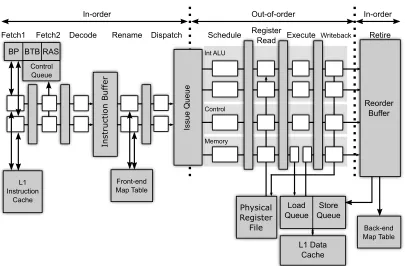
Figure 2.4An example of a canonical superscalar processor.

canonical superscalar processor.

For evaluating our design, we use FabScalar [Cho11; Dec10], which is an infrastructure of a canonical superscalar microprocessor design that includes cycle-accurate, execute-driven simulator implemented in C++ and hardware design implemented in RTL. We extend FabScalar infrastructure to implement and evaluate our design.

In FabScalar core, multiple instructions are fetched from the I-cache into multiple fetch lanes, decoded, and then stored into Instruction Buffer (IB). A set of independent pipelines pops decoded instructions from the IB, renames sources and destination registers, and then dispatches them into Issue Queue (IQ), Reorder Buffer (ROB), Load Queue (LQ) for load instructions, and Store Queue (SQ) for store instructions. When all source operands on an instruction are ready and a functional unit that is capable of executing that instruction is available, the instruction is issued into that functional unit pipeline. It then reads register operands, executes, and then writes the results back to the register file, and finally it marks itself as completed in the ROB. The core we use handles branch misprediction at the head of the ROB by flushing the pipelines.

Chapter

3

AVF-CL: AN ACCURATE

CROSS-LAYER APPROACH FOR

ONLINE ARCHITECTURAL

VULNERABILITY ESTIMATION

3.1

Introduction

In Section 2.2.1, we discuss the notion of Architectural Vulnerability Factor (AVF), which is defined as the probability that a soft error will lead to a failure. One way of estimating AVFofflineis by using Architecturally Correct Execution (ACE) analysis, described briefly in Section 2.2.2.1, and one proposed approximation scheme based on ACE analysis for predicting AVFonlineis called AVF-CL, which is introduced briefly in Section 2.2.3. In this chapter, we go in-depth about AVF-CL, an online and cross-layer approach for estimating the Architectural Vulnerability Factor of a system. A portion of this chapter is based on work published in [Wib16].

run-time AVF for the basic implementation and the optimized implementation in Section 3.6 and Section 3.7, respectively. Finally, two case studies of using AVF-CL are presented in Section 3.8 and Section 3.9.

3.2

Cross-Layer Vulnerability Estimation

AVF-CL works by taking the advantage of cross-layer information that is available at run-time to approximate the ACE analysis which is usually done post-mortem. To explain the idea of AVF-CL, we can start from how the offline ACE analysis approach works to mark whether a bit in a clock cycle is ACE or unACE, which is described in more detail in Section 2.2.2.1. Once all the bits in every clock cycle has been marked ACE or unACE, one can use Equation 2.2 to estimate AVF. For convenience, the equation is also shown in Equation 3.1.

AVF= Σeach clock cycle# of ACE Bits in clock cycle

(ACE+unACE Bits)×Total Clock Cycles (3.1) AVF-CL uses the notion ofvulnerable bitsto approximate ACE bits. Using ACE analysis, a bit can be considered unACE due to masking effects in many situations such as when a bit is currently unused, when a bit is used by instructions which will be eventually flushed without causing any side-effects, when a bit is mapped to an architectural state but will be eventually masked at algorithm-level, or even when a bit stores part of program output but any corruption on such a bit is acceptable by the user. The first two examples are approximated by the hardware predictor part of AVF-CL which is described further in Section 3.2.2. The last two examples are predicted by the means of software metadata which is discussed further in Section 3.2.1. The information from both layers is used to approximate whether a bit is vulnerableor not.

The key goal of our proposed system is to accurately compute cross-layer vulnerability online. A significant challenge toward achieving that goal is the incorporation of cross-layer information in the form of metadata. In the remainder of this section, we discuss the cross-layer metadata we leverage to compute vulnerability online, and how we organize this information into a predictor.

3.2.1 Cross-Layer Metadata

in certain live-bits are benign. This could be due to a wide variety of reasons such as logical masking, detection and correction logic, or even acceptable output error.

We want online predictors to have these same advantages but without the cost of more expensive AVF estimation approaches. We propose that most of these behaviors can be covered through two properties:livenessandimportance.

Liveness.Software can provide information about which registers, or possibly even which bits in a register, are really live and may be ACE. Liveness of registers can be computed by the compiler using well known analyses [Muc97]. Using these analyses, all dead registers can be determined to be unACE. We incorporate liveness information into metadata as the number of registers that are ACE so that the remaining ones are properly excluded as unACE at runtime. In the rest of the thesis, we refer to the number of live and possibly ACE registers as the Vulnerable Register Count (VRC).

One limitation of using liveness as an approximation of ACEness is that all the bits of a live register could be either ACE or unACE. We can live with this imprecision or try to refine it further through additional profiling or analysis. We describe an additional refinement in Section 3.4.2.2.

Importance.Another aspect of our cross-layer metadata is knowing when instructions are ACE or unACE. For example, if an instruction is protected via an optimization, like instruction duplication [Rei05b; Oh02], then it should be considered unACE. Also, if an instruction is known to be dead, then that instruction is also unACE (however, if possible, it would be more effective to eliminate it from the program).

The programmer also knows, some of the time, which code is ACE or unACE. Consider the case of resilient algorithms. For example, Monte Carlo algorithms use random sampling to carry out statistical simulations. In reality, the random numbers they generate and the computations based on them are unimportant, so long as the probability of soft error is low enough. There is no way to determine this through known compiler techniques, but such code can be labeled as unimportant by a programmer through program annotations.

We introduce the terms(un)importanceto refer to (un)ACE instructions. These are metadata markings we place on instructions. In terms of metadata,importanceis encoded as a Boolean value (a bit) that indicates whether an instruction is important or not.

Bits can't affect other instr. All bits in

a queue structure

Bits in active entries

(live)

Bits in idle/ invalid entries

Bits Used

Bits Unused

Bits used by imp. instr.

Bits used by unimp. instr.

Bits can affect other instr

Bits can't affect other instr.

Bits can affect other instr

Bits can't affect other instr. import

ant

unimportant All bits in a

register file live registers vulnerable/ important not vulnerable/ unimportant dead registers vbits

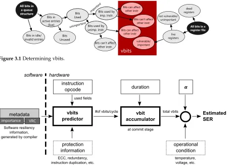
Figure 3.1Determining vbits.

metadata vbit accumulator vbits predictor importance VRC duration instruction opcode #of vbits/cycle

at commit stage hardware software total vbits 𝞪 Estimated SER Software resiliency information, generated by compiler

protection information

operational condition ECC, redundancy,

instruction duplication, etc.

temperature, voltage, etc. used fields

Figure 3.2Overall idea of AVF-CL.

3.2.2 Cross-Layer Predictor

Since soft errors in processor cores are most likely to occur in the in-core memory-based structures, we focus only on these1. The vulnerabilities of these structures are estimated by counting their ACE bits.

To determine which bits we count, illustrated in Figure 3.1, we do runtime ACE analysis that takes cross-layer metadata information into account. First, that means accurately counting based on microarchitectural and circuit-layer knowledge. In terms of processor structures, we do not count any bit that is in anidle/invalidentry of a structure. We do not count any bit that is in an active entry of a structure but isunused. This is determined by careful analysis of these structures using an RTL model of the processor.

Second, it means excluding bits specifically indicated by metadata. Specifically, we do not count bits in structures that are used by anunimportantinstruction and which cannot influence the execution of animportantinstruction. Note, we cannot just exclude the entire entry because some aspects ofunimportantinstructions could influence important ones. We discuss this more in Section 3.4.1.4. We also exclude dead orunimportantregisters as specified by metadata.

Vbits and AVF-CL. Having counted the vulnerable bits in all structures and having excluded others based on metadata, we count all that remain. These are the measured vulnerable bits or simply vbits of our predictor. We use the term vbits as our measured approximation of the true ACE-bit count that would be determined through a post-mortem analysis.

As each instruction flows through the processor, additional logic and registers track the vbits. When the instruction finally retires, it accumulates its contribution of vbits for all structures into a cumulative vbits register. If an instruction mis-speculates, its vbits are not accumulated since most of them, if not all, actually don’t matter.

We follow this basic methodology for all processor structures, register file included. The accumulated number of vbits allows us to calculate an online AVF estimate using cross-layer information, what we refer to as AVF-CL, by which we approximate the true AVF.

AVF≈AVF-CL= Σeach retiring instructionsTotal vbits of an instruction

(Total Bits)×Total Clock Cycles (3.2)

3.2.3 Accuracy with Low Overhead

In the next two sections, we discuss the two proposed designs for implementing AVF-CL in a superscalar processor. The first proposed design is the basic design which uses minimal optimization with regards to hardware overhead. The second proposed design is the optimized design that uses more approximations to reduce more overhead. In such design, a key goal is attaining high accuracy while keeping the area and power overheads of our design low. We achieve this by making simplifying approximations in the computation of vbits which have little impact on accuracy. There are two key approximations we adopted.

structure should be tracked. However, tracking all of these durations would be expensive since they all need some additional storage. Fortunately, we observe that since all queue structures, except Issue Queue, are pushed and popped in-order, instructions that are close to each other tend to have similar duration. So, seldomly tracking a few instructions’ durations gives a good approximation for the duration for all nearby instructions. A detailed description is provided in Section 3.4.1.4.

Second, computing the vulnerability of the register file is difficult. The vulnerability of a single register depends on events by different instructions. The vulnerable period starts when a physical register is written by an important instruction until its last read by another important instruction and then becomes dead. Such regions can be tracked precisely, but doing so does not provide much additional accuracy. Instead, we find it works well to directly leverage the VRC, from metadata, to approximate the vbits of the register file. We describe how we do this in more detail in Section 3.4.1.4.

3.3

Basic AVF-CL Design

This section covers the basic design of AVF-CL implementation for a superscalar processor. This section is not part of the original manuscript [Wib16] and is included here for informational purposes, especially for readers who are interested in how the AVF-CL design evolved. Readers who are interested directly in the discussion of the optimized version of AVF-CL design can skip this section.

Front-end Map Table Instruct ion Buf fer Issue Q ueue Physical Register File Reorder Buffer Back-end Map Table Int ALU Control Memory Dispatch Rename Decode

Fetch1 Schedule Register

Read Execute Writeback Retire

L1 Instruction Cache Load Queue Store Queue L1 Data Cache BP BTB RAS

Fetch2

In-order Out-of-order In-order

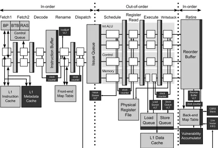
Control Queue L1 Metadata Cache clock counter InstBuff VLT Issue Queue VLT clock counter clock counter Store Queue VLT Reorder Buffer VLT Load Queue VLT clock counter Vulnerability Accumulator clock counter CSRS Stack Live Vector FIFO

Figure 3.3Simplified superscalar processor pipeline design with dark shaded blocks indicating our

modifications (components not drawn to scale).

3.3.1 Reliability Calculation Logic

In this section, we describe how to compute the reliability for each kind of structure in the processor.

3.3.1.1 Metadata Description

if either or both registers are made live; if either is live then the instruction is considered important.

Some registers are killed as a result of the change in control flow. Registers are often live-out of a basic block, but then some of them are not live-in to all successor blocks. If control flows away from a possible last use of a register, then the register is immediately dead on the next block. In order to account for these registers, we encode the extra killed registers in the metadata of the first instruction along the path on which they are killed. For our target architecture, there are 34 architectural registers: 32 general-purpose registers and loandhi registers. We assume 3 of these are always live:r0,sp, andgp. We ignore registersat, k0, k1 which are reserved for either the assembler or operating system. Hence, at most, we might need to kill 28 registers on a control flow change. We call these 28-bits thelive vector metadata and only the first instruction in each basic block has it.

Altogether, we need up to 32 bits of metadata for an instruction. Since instructions are 32 bits wide, it is easy to manage the metadata in a shadow memory space in which each instruction is given 32 bits of metadata, even though much of the space will be unused. While this is inefficient, we adopt this approach for simplicity. We expect that a variety of measures could be taken to compress the space and reduce its overhead.

Issue Queue _StampTime

1004

add r2, r1, r3

add r2, r1, r3 1004

Clock Counter

(a)

Instruction dispatched to Issue Queue; time stamp stored in entry.

(b)

Upon wake-up, the instruction leaves Issue Queue and computes total vbit occupancy.

Issue Queue Time

Stamp

1009 add r2, r1, r3 1004

Clock Counter

- x

VBit Lookup Table

I:50

250 vbits

N:34

Figure 3.4Details of Vbit calculation for the issue queue.

3.3.1.2 Occupancy-Based Structures

by the vbits required for the instruction. Figure 3.4 shows this process for the issue queue. In part (a), the instruction is dispatched and the current clock counter value is saved as the entry’s timestamp. In part (b), when the instruction wakes-up, it’s duration is computed as the difference between the clock counter value and the timestamp. The total vbits are computed by multiplying this difference with the vbits value obtained from the Issue Queue’s VBit Lookup Table.

VBit Lookup Table. The Vbit Lookup Table (VLT) contains an entry for each kind of opcode that specifies its unique vbit value. Opcodes that have the same number of vbits can be represented using a single entry. For example, all arithmetic instructions with 2 operands can be encoded into a single entry.

The VLT contains two fields used to differentiate vbits for important and unimportant instructions. We differentiate important versus unimportant vbits using the RTL of our processor; any bit that when flipped could corrupt internal processor state can never be derated without additional correction techniques. These bits remain in the AVF-CL estimate even for unimportant instructions. For example, if anaddinstruction is unimportant, it can read the wrong source register without affecting the program’s outcome, so we derate the source operands of unimportantaddinstructions. However, we cannot derate its destination register because that could lead to erroneous data flow. We performed a detailed analysis of all fields in all processor structures to determine the vbits for important and unimportant instructions. Such a procedure can be performed for any processor.

Table 3.1 shows the total number of vbits for important and unimportant instructions for a few common opcodes on the major structures in the processor. It is worth noting that unimportance has much bigger impact on some processor structures than others, to some degree limiting its impact on AVF. It is worth noting that were we to incorporate a hardware-level reliability enhancing technique, it would need a different VBit Lookup Table because it may be able to further derate these structures.

For structures that are used early in the pipeline, their vbit counts must flow with the instruction through the pipeline and ultimately be saved along side the reorder buffer for use at retirement. Fortunately, we can accumulate these values and do not need to save them separately. In the case of speculative execution, an instruction will either be fully retired or discarded, so there is no requirement to track vbits per structure separately. However, it could be useful for tracking which components are most vulnerable.