ABSTRACT
WANG, KEHUI. Combined Estimation for Quantile Regression. (Under the direction of Huixia Judy Wang and Howard Bondell.)
Quantile regression offers a convenient tool to assess the relationship between a re-sponse and covariates in a comprehensive way and it is appealing especially in applications where interests are on the tails of the response distribution. However, due to data spar-sity, the finite sample estimation at tail quantiles often suffers from high variability. To improve the tail estimation efficiency, we consider modeling multiple quantiles jointly for the cases where the quantile slope coefficients appear constant within a small quantile region at tails.
Combined Estimation for Quantile Regression
by Kehui Wang
A dissertation submitted to the Graduate Faculty of North Carolina State University
in partial fulfillment of the requirements for the Degree of
Doctor of Philosophy
Statistics
Raleigh, North Carolina 2015
APPROVED BY:
Ana-Maria Staicu Yichao Wu
Huixia Judy Wang
Co-chair of Advisory Committee
Howard Bondell
DEDICATION
BIOGRAPHY
ACKNOWLEDGEMENTS
First, I would like to thank my advisor, Dr. Huixia (Judy) Wang. I am grateful for her immense help, great patience, and inspiring work attitude. This dissertation would not have been possible without her guidance. I have the highest regard for her deep understanding of statistics and the qualities of being professional and self-discipline. It has been a great pleasure working with her, and I have learned so much beyond research but more broadly for my future career.
I would also like to thank all my committee members, Howard Bondell Ana-Maria Staicu and Yichao Wu, for being supportive during the entire process. Their careful review, valuable comments and suggestions helped strengthen this dissertation. I also thank Huaiyu Dai for serving on my committee as the graduate school representative.
I would like to extend my sincere thanks to Ana-Maria Staicu and Arnab Maity, with whom we collaborate in the functional quantile linear regression project. I am grateful for all the mentorship and advices provided by them. My appreciation also goes to the DGPs of the department, Sujit Ghosh, Howard Bondell and Keem Weems, who are always ready to help. I should also thank all the staff , for their excellent service to the department.
My appreciation goes to Ellen Lentz, my supervisor at Genentech, and Veena So-mayaji, my supervisor at Pfizer. They led me into the pharmaceutical industry and provided invaluable guidance to my future career.
I thank Yifang Li, Tian Chen, Liwei Wang and Bo Zhang and Changning Niu, for being my true friends of life.
Special thank to my father, who inspired me in the first place for higher education, and made me never give up. The same goes to my mom and sister, without whose unconditional love and accompany I couldn’t come this far. Last but not least, I have the heartiest gratitude to my husband and best friend Meng Li. We have been through all the good times and bad times together. Life has been changed, but I’m glad that you are always there for me.
TABLE OF CONTENTS
List of Tables . . . vii
List of Figures . . . ix
Chapter 1 Introduction . . . 1
1.1 Introduction to Quantile Regression . . . 1
1.2 Introduction to Combined Quantile Regression . . . 2
1.3 Introduction to Functional Data Analysis . . . 4
Chapter 2 Combined Estimation for Tail Quantile Regression . . . 6
2.1 Introduction . . . 6
2.2 Proposed Methods . . . 8
2.2.1 Joint Quantile Regression Model . . . 8
2.2.2 Optimally Weighted Quantile Average Estimator . . . 10
2.2.3 Weighted Composite Quantile Estimator . . . 12
2.2.4 Estimation of EVI . . . 16
2.2.5 Comparison of Asymptotic Efficiency . . . 17
2.3 Simulation Study . . . 19
2.4 Application to Chicago Precipitation Data . . . 22
2.5 Proof . . . 24
Chapter 3 Combined Estimation for Conditional Value-at-Risk . . . 35
3.1 Introduction . . . 35
3.2 CAViaR Model . . . 37
3.3 Combined Quantile Regression . . . 38
3.3.1 Composite Quantile Loss Function . . . 38
3.3.2 Asymptotic Property . . . 39
3.4 Computation . . . 40
3.5 VQR test . . . 42
3.6 Simulation . . . 45
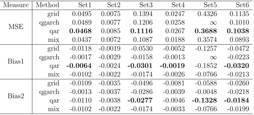
3.6.1 Choices of Initial Values for the Conventional CAViaR Estimator 45 3.6.2 Comparison of Local (Conventional) Estimation and Composite Estimation . . . 47
3.6.3 Assessment of Goodness of Fit via VQR Test . . . 48
3.7 Data Application . . . 49
3.8 Proof of Theorem 3.3.1 . . . 53
Chapter 4 Inference in Functional Linear Quantile Regression . . . 60
4.1 Introduction . . . 60
4.2.1 Hypothesis tests in functional quantile regression model . . . 62
4.2.2 Estimation procedure . . . 65
4.2.3 Wald-type test statistic . . . 66
4.3 Asymptotic results . . . 66
4.3.1 Assumptions . . . 66
4.3.2 Asymptotic distributions . . . 67
4.3.3 Estimation of p0 . . . 69
4.4 Simulation . . . 70
4.5 Application . . . 74
4.6 Proofs . . . 77
4.6.1 Proof of Theorem 4.3.1 . . . 77
4.6.2 Proofs of Lemmas . . . 80
LIST OF TABLES
Table 2.1 The asymptotic relative efficiency of QAE, CRQ, WCRQ+ and OWCRQ with respect to OWQAE (OWCRQ) for five types of dis-tributions. . . 18 Table 2.2 Optimal weights for the WCRQ and WQAE methods atτk = 0.95,
0.96, 0.97, 0.98 and 0.99. . . 18 Table 2.3 The 103×MSE of different estimators ofβ in Example 1. The values
in the parentheses are the standard errors of 103×MSE. . . . 21
Table 2.4 The 103×MSE of different estimators ofβ in Example 2. The values
in the parentheses are the standard errors of 103×MSE. . . 21 Table 2.5 The 103×MISE of different estimators in Example 3. The values in
the parentheses are the standard errors of 103×MISE. . . . 22
Table 2.6 The upper part of the table summarizes the estimated common slope b
β for the proposed methods and the bootstrap standard error (s.e.). The lower part of the table presents the quantile-specific weights given by different methods based on the estimated extreme value index ˆξ= 0.29. . . 24 Table 2.7 The prediction error of different methods at quantile levels 0.990,
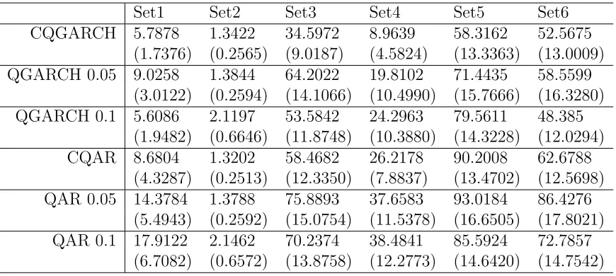
0.992 and 0.995. The values in the parentheses are the standard errors. 25 Table 3.1 The MSE, Bias1 and Bias2 of 4 methods using different initial values. 47 Table 3.2 The 1000× MSE of the estimated 0.05-th quantiles for composite
and local estimations. The 1000×standard errors are reported in the parentheses. . . 49 Table 3.3 The 1000× MSE of the estimated 0.1-th quantiles for composite
and local estimations. The 1000× standard errors are reported in the parentheses. . . 49 Table 3.4 The 100×MSE of the composite and local estimations of the
com-mon parameter β. The 100× standard errors are reported in the parentheses. . . 50 Table 3.5 The size of VQR test at 5% and 10% quantiles. The nominal levels
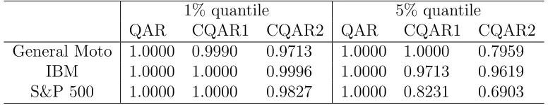
are 0.1 and 0.05. . . 50 Table 3.6 The p-values of the VQR test for different methods on three data sets. 51 Table 3.7 Local and composite CAViaR estimators for the General Motor data. 52 Table 3.8 Local and composite CAViaR estimators for the IBM data. . . 52 Table 3.9 Local and composite CAViaR estimators for the S&P 500 data. . . 52 Table 4.1 Type I error rates of the functional Wald-type test at given
Table 4.2 Type I error rates of the functional Wald-type test at given signifi-cance levelsα when considering U2 ={0.1,0.2,0.6,0.7}. . . 72
Table 4.3 Type I errors when using the method of the naive multivariate quan-tile regression (NMQR), the mean as the scalar summary (SSQR) and Multivariate PCA (MPCA). When one method returns error (due to singularity of the design matrix) in more than 20% replica-tions, we report it as “NA”. . . 72 Table 4.4 Bootstrap standard errors of the estimates of 4 coefficients including
the interceptβ0 from the QAE, CRQ and the local quantile
regres-sion estimation at the 0.9-th quantile (RQ). The method of FPCA selects 3 PC’s for all 1000 bootstrap samples. . . 76 Table 4.5 Mean prediction errors from different methods over 1000
LIST OF FIGURES
Figure 2.1 Local quantile regression estimates of the slope at upper quantiles for the precipitation data in Aurora station. . . 23 Figure 4.1 Powers of FPCA and SSQR in various scenarios. . . 73 Figure 4.2 Hourly bike rentals for casual users. Thex-axis is the hour and the
Chapter 1
Introduction
1.1
Introduction to Quantile Regression
In statistics, regression is an important technique to model the relationship between response (dependent variable) and predictors (covariates or independent variables). The traditional estimation is the ordinary least squares (OLS), which estimates the parameters by minimizing the sum of squared errors. Consider a linear regression model
yi =xTiβ+i, i= 1, . . . , n,
where yi is the response, xi is the p-dimensional predictor, β is the p-dimensional pa-rameter, andi is the error with mean 0. The OLS estimation of β is defined as:
b
β= arg min
β∈Rp
n X
i=1
(yi−xTβ)2.
The OLS estimator has a closed form βb = (XTX)−1XTY, whereX = (x1, . . . ,xn)T is the design matrix and Y = (y1, . . . , yn)T is the vector of responses.
et al., 2005) and in financial risk management (Chernozhukov and Du, 2008).
Quantile regression, first introduced by Koenker and Bassett (1978), was a valuable alternative to the OLS. Different from the OLS, quantile regression models the conditional quantile of the response as a function of the predictor. Let Y be the scalar response variable,X be thep-dimensional vector of predictors, and{(yi,xi)}n1 be a random sample
of (Y,X). For a given quantile level τ ∈ (0,1), consider the linear quantile regression model
QY(τ|xi) =α0(τ) +xTi β0(τ),
where QY(τ|x) = inf{y : FY(y|x) ≥ τ} is the τ-th conditional quantile of Y given
X =x, and FY(·|x) is the conditional distribution function. The conventional quantile regression estimator of the parametersα0(τ) and β(τ) is defined as:
{α(τ),b βb(τ)}= arg min
(α,β)∈Rp+1
n X
i=1
ρτ(yi−α−xTi β), (1.1)
where ρτ(t) = t{τ − I(t ≤ 0)} is the quantile loss function and I(·) is the indicator function. The objective function is minimized via linear programming.
Quantile regression offers a convenient tool to access the relationship between a re-sponse and covariates in a comprehensive way by varying the quantile level τ. Conse-quently, quantile regression is appealing especially in applications where interests are on the tails of the response distribution.
1.2
Introduction to Combined Quantile Regression
Combined estimation was first proposed by Hogg (1980), and some asymptotic proper-ties of the combined estimators were studied by Koenker (1984). Consider the classic independent and identically distributed (i.i.d.) error model
yi =α0 +xTi β0+i, i= 1, . . . , n,
which implies
QY(τ|xi) = α0(τ) +xTi β0, (1.2)
Note that the above model (1.2) implies that the quantile intercept α0(τ) is varying
across different τ, while the slope is a constant. This equal slope feature motivates the estimation of the common slope by combining information across multiple quantiles.
Consider K quantile levels 0< τ1 < . . . , τK <1, the vector of true parameters isθ0 =
{α0(τ1), . . . , α0(τK),βT0}T. There are two ways to aggregate information across quantile
levels. Koenker (1984) proposed the weighted quantile average estimator (WQAE). First, we obtain quantile regression estimators by minimizing the quantile loss function in (1.1) at τ1, . . . , τK separately. Each βb(τk), k = 1, . . . , K is a consistent estimator of β0, and the WQAE estimator of the slope is defined as
b
βW QAE = K X
k=1
$kβb(τk),
where $k is the weight assigned to quantile levelτk and Pk$k = 1.
Hogg (1980) proposed the weighted composite regression of quantile (WCRQ) estima-tor, which is obtained by minimizing the weighted average of the quantile loss function
b
α(τ1), . . . ,α(τb K),βb
= arg min
(α1,...,αK,β)∈RK+p
K X
k=1
n X
i=1
ωkρτk(yi−αk−x
T
i β), (1.3)
where ωk is the weight corresponding to τk and P
kωk= 1.
1.3
Introduction to Functional Data Analysis
Recent development of technology and computational capacity allows us to record data with repeated measurement in high frequency, making it natural to conceptually regard data as a function. In functional data analysis (FDA), the data is viewed as a realization of an underlying random process X(t) in L2(T), where L2(T) is the L2 space onT and T ⊂R is a bounded closed interval.
Suppose we have n i.i.d. observations {X1(t), X2(t), . . . , Xn(t) : t ∈ T }, where
E{Xi(t)} = µ(t) and Cov{Xi(s), Xi(t)} = G(s, t), i = 1, . . . , n. It is well known that the covariance kernel K(s, t) has orthogonal expansion K(s, t) = P∞
j=1λjφj(s)φj(t),
where the eigenvalues λj are nondecreasing and nonnegative, and φj’s are the associ-ated eigenfunctions. Here {φj : j = 1· · · ,∞} forms an orthnomal basis of L2(T). Then by Karhunen-Lo´eve expansion, the random processXi(t) can be represented as
Xi(t) =µ(t) +
∞
X
j=1
zi,jφj(t), (1.4)
where zi,j = R1
0{Xi(t)−µ(t)}φj(t)dt is the so-called principle scores (PC’s) for Xi
satis-fying that E(zi,j) = 0, Var(zi,j) =λj and E(zi,jzi,j0) = 0 (j 6=j0).
For each individual functional data, what we actually observe are mi discrete mea-surements with measurement error at time point t1, . . . , tmi ∈ T, denoted as
Wi,j =Xi(ti,j) +i,j, i= 1, . . . , n, j = 1, . . . , mi,
where the measurement error i,j has mean 0 and variance σ2w.
Dimension reduction is critical in FDA, and among various methods, functional prin-cipal component analysis (FPCA) is the most widely used technique. Given the observed data {Wij, i = 1, . . . , n, j = 1, . . . , mi}, one can first estimate the mean and covariance kernel function via commonly used smoothing techniques such as local polynomial. Then with the estimated eigenfunctions φbj(t), we can recover the scores zi,j by
b
multivariate setting.
Functional quantile regression (fQR) model is an extension of the standard linear quantile regression to functional covariates. We consider the i.i.d. data of (Yi, Xi), where Yi is a scalar response variable and Xi = Xi(t), t ∈ T is a random covariate function. Then we assume that (Yi, Xi) is generated from the following model
Yi =α(τ) + Z 1
0
β(t, τ)Xic(t)dt+i (1.5)
whereβ(·, τ)∈L2(T),Xic(t) =Xi(t)−E{Xi(t)}and theτth quantile of the i.i.d. random error i is 0. Let QY|X(τ) be the conditional τ-th quantile function of Y given X for a given τ, then equation (1.5) implies that
QYi|Xi(τ) =α(τ) +
Z 1
0
β(t, τ)Xic(t)dt, (1.6)
which is the fQR model.
The coefficient functionβ(t, τ) can be expanded by the eigenfunction basis asβ(t, τ) = P∞
k=1βj(τ)φj(t), whereβj(τ) =
R1
0 β(t, τ)φj(t)dt. Suppose we havepnPC’s to be selected,
then the fQR model is reduced to
Q(pn)
Yi|Xi(τ) = α(τ) +
pn
X
j=1
βj(τ)zi,j.
Chapter 2
Combined Estimation for Tail
Quantile Regression
2.1
Introduction
Quantile regression has generated tremendous research interests after being introduced by Koenker and Bassett (1978). Different from the conventional least squares regression, quantile regression models the τth conditional quantile of the response as a function of the covariates, where 0< τ <1 is the prespecified quantile level of interest.
An important problem in many fields is to model rare and extreme phenomena, which correspond to the lower or upper tails of the variable. For instance, in environmental studies, extremely low or high precipitations are of more importance than average pre-cipitations, since hydrologists may want to model the chance of draught to help with the design of reservoirs, and model the chance of heavy rainfall to help with the design of flood drains (Pandey and Nguyen, 1999; Friederichs and Hense, 2007; Friederichs, 2010; Wang et al., 2012). In the analysis of infant birth weights (Abrevaya, 2002), extremely low birthweights are associated with various health problems and higher infant mor-tality rates. In financial risk management, investors are more interested in forecasting extremely large financial losses of an institution’s portfolio given today’s available infor-mation (Chernozhukov and Du, 2008). Without loss of generality, in this paper, we focus on high quantile regression.
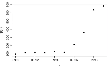
fitting the regression model at one quantile level at a time, the conventional quantile regression, also referred to as the local quantile regression thereafter, is often unstable at tails. In applications where the covariate effects have some common features across quantile levels in the tail region, it is desirable to aggregate information across multiple quantiles to improve the estimation efficiency over the local quantile estimator (i.e. ventional quantile-specific estimator). For instance, Figure 4.1 in Section 4 plots the con-ventional quantile regression estimates of slopes at multiple quantiles, where the response is the observed daily precipitation in Chicago area and the predictor is the simulated daily precipitation from the ERA-40 reanalysis model. The estimated quantile slopes appear to be constant in the upper quantiles τ ∈ (0,990,0.995). For such data sets, we could utilize the commonality of quantile slopes to improve the estimation efficiency at tails by pooling information across tail quantiles.
Consider a linear regression model with quantile-invariant covariate effects, there exist two plausible ways to combine information across quantiles: combining the local quantile estimators or the criterion functions involved in the estimation procedure at different quantiles. The first strategy leads to the weighted quantile average estimator (WQAE) introduced by Koenker and Bassett (1978), which is the weighted average of quantile-specific slope estimators. The second strategy leads to the weighted composite regression of quantiles (WCRQ) estimator first proposed by Hogg (1980), which minimizes the combined quantile objective function across quantiles. For central quantiles with 0< τ < 1, Koenker (1984) studied the asymptotic properties of these two estimators and showed their asymptotic equivalency when optimal weights are used. In recent years, combined quantile regression has been studied in various setups with more work focusing on the first strategy. The composite quantile regression idea was employed for estimation and variable selection in linear regression (Zou and Yuan, 2008; Tang et al., 2012a), nonlinear regression (Jiang et al., 2012c), nonparametric regression (Kai et al., 2010, 2011; Guo et al., 2012; Jiang et al., 2012b, 2013b), and linear regression with censored data (Jiang et al., 2012a; Tang et al., 2012b). Based on the combined quantile loss function, Jiang et al. (2013a) proposed two penalization methods that perform estimation, detection of the interquantile slope commonality and variable selection simultaneously. Zhao and Xiao (2014) discussed both WCRQ and WQAE methods for linear and nonparametric regression models.
quan-tiles with τ ∈ [,1−], where 0 < < 1 is some positive constant, and this rules out the study of extreme tails of the response distribution. To our knowledge, there exists no discussion about how to optimally combine information across tail quantiles. At the tails with quantile level τ → 1 as the sample size n → ∞, the convergence rate of quantile regression estimator depends on the heaviness of the tails of the response distribution and is slower than root-n. Therefore, the methods and theory developed in Koenker (1984) and Zhao and Xiao (2014) are not applicable for tail quantiles. In this paper, using the tools of extreme value theory, we establish the asymptotic properties of the weighted com-posite and weighted quantile average estimators for tail quantile regression, and propose a procedure for estimating the optimal weights for both estimators.
The rest of this chapter is organized as follows. In Section 2, we propose two weighted estimators for tail quantile regression with constant slopes, present their asymptotic properties and discuss the construction of optimal weights. The numerical performance of the proposed estimators is assessed through a simulation study in Section 3 and the analysis of a daily precipitation data in Chicago area in Section 4. All technical details are provided in the Appendix.
2.2
Proposed Methods
2.2.1
Joint Quantile Regression Model
Let Y be the scalar response variable, X be the p-dimensional vector of covariates, and {(yi,xi)}n1 be a random sample of (Y,X). Suppose we are interested in regression at the upper tails with quantile level τ ∈ T = [1−n,1], where n →0 as n→ ∞. Let FY(·|x) denote the conditional distribution function of Y given x. The linear quantile regression model assumes that
QY(τ|x) = α0(τ) +xTβ0(τ), τ ∈ T, (2.1)
whereQY(τ|x) = inf{y:FY(y|x)≥τ}is theτth conditional quantile ofY givenX =x, and α0(τ)∈R andβ0(τ)∈Rp are the unknown quantile coefficients associated with the
τth quantile level.
(α(τ),β(τ)) is defined as
b
α(τ),βb(τ)
= argmin(α,β)∈Rp+1
n X
i=1
ρτ(yi−α−xTi β), (2.2)
where ρτ(t) = t{τ − I(t ≤ 0)} is the quantile loss function and I(·) is the indicator function (Koenker, 2005). The conventional quantile regression method estimates the quantile coefficient at each quantile level of interest separately, and the resulting local slope estimator βb(τ) can vary freely in τ. However, in data-sparse area such as extreme tails, the variability of local estimates is often overly high. In some applications it might be reasonable to assume the slope coefficient β(τ) to share some common features, for instance, to be constant or locally linear, within a certain region of quantiles. By utilizing this commonality, we can aggregate information across quantiles to improve the estima-tion efficiency. In this paper, we focus on linear quantile regression with constant slopes at the upper tails, but the proposed method can also be easily extended to lower tails, and also be adapted to accommodate other common features such as local linearity, and cases where only a subset of the components of β(τ) are locally constant.
We assume the following linear quantile regression model at the upper tails
QY(τ|x) = α0(τ) +xTβ0, τ ∈ T. (2.3)
Different from model (2.1), here the quantile slope is assumed to be constant at the upper tails across τ ∈ T, but α(τ) is still an increasing function ofτ.
2.2.2
Optimally Weighted Quantile Average Estimator
For model (2.3) at K upper quantiles, the unknown parameters consist of K distinct interceptsα0(τk) and one common slope vectorβ0. Denote the vector of true parameters θ0 = (α0,1, . . . , α0,K,βT0)T, whereα0,k =α0(τk), k = 1, . . . , K.
Let $k be the weight assigned to the quantile level τk, k = 1, . . . , K. For the sake of identifiability, we assume that 1TK$ = 1, where $ = ($1, . . . , $K)T, and 1K denotes a K-dimensional vector of ones. We define the weighted quantile average estimator ofθ as
b
βWQAE = K X
k=1
$kβb(τk), (2.4)
where ˆβ(τk) is the local quantile slope estimator obtained by minimizing the objective function in (2.2) at the τkth quantile. The WQAE is the weighted average over conven-tional estimators at multiple high quantiles, and thus can be viewed as a special case of the L-estimator with discrete weights. Portnoy and Koenker (1989) and Koenker (1984) studied the L-estimator for the slope in the location-shift linear model, which implies that β(τ) is constant across the entire quantile regionτ ∈(0,1).
The asymptotic properties of WQAE at central quantiles have been studied by Koenker (1984) and Zhao and Xiao (2014). In the following Theorem 2.2.1, we establish the asymptotic distribution of βbW QAE at tails.
For any sequences a(z) and b(z), throughout the paper, we use the notation a(z) ∼ b(z) to mean thata(z)/b(z)→1 as a specified limit is taken overz. We make the following assumptions.
A1. The distribution function FY(y|xi) is absolutely continuous with continuous den-sity fY(y|xi), which is uniformly bounded away from zero and infinity and has a bounded first derivative around QY(τk|xi) for anyk = 1, . . . , K.
A2. The distribution of X has a compact support X. The expectation E(X) =0, and E(XXT) = D exists and is positive definite.
A3. LetU =Y −XTβ0. There exists some distribution functionF0(·) in the maximum
domain of attraction with extreme value indexξ, such that 1−FU(z|x)∼1−F0(z)
asz →su uniformly inx∈ X, where su is the upper end-point of U.
A5. Fork = 1, . . . , K, (1−τk)/(1−τ) =lk+o(1) for some τ →1 and n(1−τ)→ ∞, where lk >0 are constants.
Condition A1 specifies some conditions on the conditional distribution of Y, which are standard in quantile regression. Condition A2 assumes that the covariate vector X has mean zero. In general, for cases whereE(X) is not zero, one can simply center the covari-ate to have mean zero before carrying out the data analysis. Conditions A3-A4 specify some assumptions on the tail behaviors of the conditional distribution of Y, which are needed to establish the properties of the quantile coefficient estimator at tails. Specifi-cally, A3 requires that after the linear transformation,U =Y −XTβ0 is tail equivalent to a distribution F0 in the maximum domain of attraction. The domain of attraction
assumption is not very restrictive since it covers most of the common distributions such as Gaussian, Beta, and t distribution, and so on; see de Haan and Ferreira (2006) for more details about the domain of attraction. ConditionA4is a von Mises type condition, which specifies how the density function decays at the right tail. The von Mises condition is basic for a distribution to belong to the maximum domain of attraction.
Condition A5 restricts our attention to the intermediate order of extreme quantiles with τk→1 and n(1−τk)→ ∞ asn → ∞.
Remark 1. Extreme value index ξ is a measurement of the heaviness of the tail distribution. According to the signs of the extreme value indices, distributions in the domain of attraction can be categorized into 3 classes: heavy-tailed, light-tailed and short-tailed. A distribution withξ >0 has infinite right endpoint and a heavy tail. While a distribution withξ= 0 also has infinite right endpoint but the tail is light. As forξ <0, the right endpoint of the distribution is −1/ξ, so the distribution has a short tail. For more details about extreme value index, we refer to de Haan and Ferreira (2006, chapter 1).
Throughout this paper, we define
an=
p
(1−τ)n F0−1(τ)−F0−1(τem)
, where eτm = 1−m(1−τ) for some m >1.
($1, . . . , $K)T, as n → ∞, we have
an(βbW QAE−β) d
→ N 0, σW QAE2 ($)
m−ξ−1 −ξ
−2
D−1
! , σW QAE2 ($) = $TΦ−1(ξ)ΓΦ−1(ξ)$,
where Γ is a K × K matrix with the (k, k0)th element as min(lk, lk0), Φ(ξ) = diag{(l1ξ+1, . . . , lKξ+1)}, and D =E(XXT).
Theorem 2.2.1 suggests that the asymptotic covariance of βbW QAE depends on the weights $ only through a scalar σ2
W QAE($), which is a function of $. Therefore, the optimal weights that maximize the efficiency of βbW QAE is
$opt = argmin$$TΦ
−1(ξ)ΓΦ−1(ξ)$, subject to1T
K$ =1. (2.5)
The minimization in (2.5) is a standard constrained optimization problem. Direct appli-cation of the Lagrange multipliers method gives
$opt = Φ(ξ)Γ−1φ(ξ){φT(ξ)Γ−1φ(ξ)}−1. (2.6)
Therefore, the minimal value of σ2
WQAE is {φ
T(ξ)Γφ(ξ)}−1. We refer to the optimal
WQAE of β0 based on $opt as βbOWQAE.
2.2.3
Weighted Composite Quantile Estimator
An alternative estimator of the common slope β is the weighted composite regression of quantiles (WCRQ) defined as
b
θW CRQ = argmin α1,...,αK,β
K X
k=1
ωk n X
i=1
ρτk(yi−αk−x
T
i β), (2.7)
whereωkis the weight assigned to the quantile levelτk. The estimatorθbW CRQis referred to as the weighted composite regression of quantiles (WCRQ) estimator, since it minimizes the weighted joint quantile objective function across quantile levels.
considered a combined quantile objective function that is similar to the one in (2.7) but assigns equal weights to different quantiles. However, since neighboring quantiles are correlated especially at the tails, in general assigning equal weights is not an efficient way to combine information across quantiles. In some cases, composite estimator based on equal weights could even be less efficient than the local quantile estimator obtained at a single quantile level. Therefore, it is important to select appropriate weights ωk in order to achieve efficiency gain.
Note that when the components in ωopt are non-negative, the combined objective
function in (2.7) is convex. The optimization in (2.7) can be recast into a linear program-ming problem and solved by using existing software such as the function “make.lp” in the R package lpSolveAPIor function “rq.fit.fnb” in the R package quantreg. But when some weights are negative, the objective function in (2.7) might not be convex and will lead to difficulty in minimization. Therefore, to avoid potential computational difficulty, we first consider WCRQ with nonnegative weights. The following theorem establishes the asymptotic properties of the weighted composite estimator at tails with given nonnegative weights.
Theorem 2.2.2 Suppose that model (2.3) and conditions A1-A4 hold, and ωk ≥0 for k = 1, . . . , K, as n→ ∞,
an(bβW CRQ−β0)
d
→ N 0, σ2W CRQ(ω)
m−ξ−1 −ξ
−2
D−1
! , σW CRQ2 (ω) = {ωTφ(ξ)}−2ωTΓω,
where φ(ξ) = (l1ξ+1, . . . , lKξ+1)T.
Sub-optimal Estimator. Similar to WQAE, the optimal weights for WCRQ can be obtained by minimizing the asymptotic variance of βbW CRQ, which depends on the weights only through a scalar σ2
W CRQ(ω). We define
ωsub = argminω1≥0,...,ωK≥0{ω
Tφ(ξ)}−2ωTΓω, subject to 1T
Kω =1. (2.8)
We refer to ωsub as the sub-optimal vector of weights since it minimizes the asymptotic
pro-gramming software such as the function “solve.QP” in the R packagequadprog. Through-out, we denote the minimizer of (2.7) based on ωsub as bθWCRQ+.
Compared with OWQAE, the additional restriction in WCRQ+ estimator may cause some loss of efficiency for the estimation of β as indicated in Proposition 2.2.1; also see some numerical evidences in Section 2.5. If we release the nonnegative constraint, we can obtain the “optimal” weight that minimizesσ2
W CRQ as ωopt =Γ−1φ(ξ)/{1TKΓ
−1
φ(ξ)}. (2.9)
Recall that the minimum value ofσ2W QAEis{φT(ξ)Γφ(ξ)}−1, which is the same as that of
the OWQAE estimator. Note that ωToptφ(ξ) = φT(ξ)Γ−1φ(ξ)≥ 0. Following the similar argument as in the proof of Theorem 2.2.2, we can show that the asymptotic normality in Theorem 2.2.2 still holds for the WCRQ estimator based on the weights ωopt, and
this estimator has the same asymptotic variance with OWQAE. Thereafter, we refer to the WCRQ estimator based on ωopt as the OWCRQ (optimally weighted composite
regression of quantile).
Proposition 2.2.1 For any weight ω ∈ RK, σ2
W CRQ(ω) ≥ {φ
T(ξ)Γφ(ξ)}−1, and the
equality holds if and only if ω =ωopt.
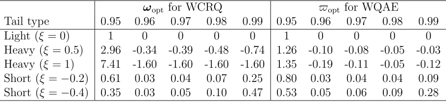
Remark 2.In some situations, upper quantiles may be negatively correlated, resulting in negative optimal weights. In such cases, using WCRQ based on sub-optimal weights is not as as efficient as the OWCRQ based on the optimal weights or the OWQAE estimator. For tail quantile regression, we find out that the occurrence of negative optimal weights depends on the heaviness of the tail of the response distribution. Using linear algebra, we can show that when the response distribution is heavy-tailed with ξ > 0, the least extreme quantile will receive positive weight and all the others receive negative weights. For light-tailed distributions withξ = 0, asτ →1, all the weights will be put into the least extreme quantile levelτ1 while other higher quantiles receive zero weight. For short-tailed
distributions withξ < 0, all the weights at high quantiles are positive. Some justification for the above findings are provided in the Appendix. For illustration, Table 2.2 presents the optimal weights for normal, t2, t1, Beta(2, 5) and Beta(2, 2.5) distributions, which
are in the domain of attractions with ξ = 0,0.5, 1, -0.2 and -0.4, respectively.
One-step Estimator. When ωopt contains negative weights, the weighted objective
OWCRQ estimator. To utilize the optimal weights ωopt and meanwhile avoid the
non-convex optimization, we consider an alternative one-step estimator. Letzi,k = (eTk,xTi )T, where ek is aK-dimensional vector with the kth entry equals 1 and the others equal 0. Denote
A(θ) = K X
k=1
n X
i=1
ωk(o)zi,k{I(yi−zTi,kθ<0)−τk}, B(θ) = K X
k=1
n X
i=1
ω(ko)zi,kzTi,kfY(zTi,kθ|xi),
where ω(ko) is the kth element of ωopt. The one-step estimator of θ0 is defined as
b
θOS=eθ− n
B(eθ)o
−1
A(eθ), (2.10)
where eθ is any an-consistent estimator ofθ0.
The one-step estimating approach was first discussed by Bickel (1975) for estimating the location parameter in a linear model. Recently, Bradic et al. (2011) studied the one-step method for variable selection based on penalized composite quasi-likelihood. Following the similar arguments as in Bradic et al. (2011), we can show that for tail quantiles, the one-step slope estimator βbOS achieves the same asymptotic efficiency as the OWQAE and OWCRQ estimator as long as the initial estimator βe is consistent of the same rate an.
Theorem 2.2.3 Suppose conditionsA1-A5 hold, if||eθ−θ0||=Op(1/an), then we have
an(bβOS−β0)
d
→N 0, 1
φT(ξ)Γφ(ξ)
m−ξ−1 −ξ
−2
D−1
! .
Note that to achieve the above asymptotic efficiency, the initial estimator eθ can be any an-consistent estimator such as the conventional quantile regression estimator or b
θW CRQ with any given nonnegative weights. In the implementation, we use θbW CRQ+ as the initial estimator.
estimate the quantity
n X
i=1
zi,kzTi,kfY(zTi,kθ|xi)
by using the kernel method proposed by Powell (1991). Our numerical investigation suggests that these two methods work well for large sample sizes but they sometimes lead to unstable results for small samples. Note that model (2.3) and assumption A3
imply that as τ → ∞, fY{QY(τ|x)|x} = fU{α(τ)|x} ∼ f0{α(τ)}, which is common
acrossx. Therefore, we suggest to use the nonparametric kernel density estimation based on the estimated residuals bi =yi−xTi βbW CRQ+ as in Zhao and Xiao (2014).
Different from the WCRQ estimator that requires minimizing the weighted combined quantile objective function, the calculation of WQAE only requires minimizing the convex quantile objective function in (2.2) at each quantile levelτkseparately. Therefore, negative weights in$opt do not cause any computational difficulty. In contrast, the WCRQ method
requires solving the combined objective function of K +p parameters, and a one-step iteration is needed for calculating the optimal estimator when some of the optimal weights are negative. Despite the possible computational complication, the WCRQ method has the following advantages. First, the weighted composite quantile regression method can be used to accommodate general interquantile commonality in a more direct way, for instance, locally linear quantile slopes with β(τk) = β(τ1) + (τk−τ1)γ, where γ is an
unknown parameter. Second, penalization can be incorporated in the weighted composite quantile loss function for variable selection and inter-quantile shrinkage; see for instance Bradic et al. (2011), Jiang et al. (2013a) and Jiang et al. (2014).
2.2.4
Estimation of EVI
can be written as
g(z|Ψ) =
1
σ n
1 + ξ(zσ−u)o
−(1+ξ)/ξ
, if ξ6= 0,
1
σ exp{−(z−u)/σ}, if ξ= 0, where z > ufor ξ≥0 and 0≤z−u≤ −σ/ξ for ξ <0.
In our setup, we define ui = QbY(τ0|xi), i = 1, . . . , n, where τ0 → 1 as n → ∞, and b
QY(τ0|x) is any consistent estimator ofQY(τ0|x), for instance, the conventional quantile
regression estimator. We can then estimate ξ by maximizing the GPD likelihood based on the exceedances {yi −ui : yi ≥ ui, i = 1, . . . , n}. If F0(·) satisfies the second-order
condition as defined on page 44 of de Haan and Ferreira (2006) and ξ > −1/2, it then follows by Smith (1987) and Theorem 3.4.2 in de Haan and Ferreira (2006) that the maximum likelihood estimator ofξ is consistent and asymptotically normal. Throughout our numerical studies, we chooseτ0 = 0.95 and obtain the maximum likelihood estimator
of ξ by using the function “gpd.fit” in the R package ismev.
2.2.5
Comparison of Asymptotic Efficiency
Theorems 2.2.1 and 2.2.2 suggest that the OWCRQ and OWQAE estimators are asymp-totically equivalent. The one-step estimator βbOS achieves the same asymptotic efficiency as OWCRQ. The WCRQ+ estimator is the same as OWCRQ when the optimal weights are all nonnegative, but the former is asymptotically less efficient when some of the optimal weights are negative.
We assess the efficiency gain of using optimal weights by comparing the asymptotic efficiency of OWCRQ/OWQAE, WCRQ+ with CRQ and QAE, the composite and quan-tile average estimators based on equal weights. We consider five different cases: ξ = 0 corresponding to light-tailed such as exponential and normal distributions, ξ = 0.5 and 1 corresponding to heavy-tailed distributions such as t2 and t1, ξ=−0.2 and -0.4
corre-sponding to short-tailed distributions such as Beta(2, 5) and Beta(2, 2.5). We consider five quantiles with τk = 0.95,0.96,0.97,0.98 and 0.99. Table 2.1 summarizes the asymptotic relative efficiency of QAE, CRQ and WCRQ+ with respect to OWQAE (or equivalently OWCRQ), and Table 2.2 presents the optimal weights for both the WCRQ and WQAE methods.
Table 2.1: The asymptotic relative efficiency of QAE, CRQ, WCRQ+ and OWCRQ with respect to OWQAE (OWCRQ) for five types of distributions.
Tail type QAE CRQ WCRQ+
Light (ξ = 0) 0.64 0.81 1.00 Heavy (ξ = 0.5) 0.23 0.52 0.90 Heavy (ξ = 1) 0.06 0.33 0.77 Short (ξ =−0.2) 0.84 0.92 1.00 Short (ξ =−0.4) 0.95 0.95 1.00
Table 2.2: Optimal weights for the WCRQ and WQAE methods atτk = 0.95, 0.96, 0.97, 0.98 and 0.99.
ωopt for WCRQ $opt for WQAE
Tail type 0.95 0.96 0.97 0.98 0.99 0.95 0.96 0.97 0.98 0.99
Light (ξ = 0) 1 0 0 0 0 1 0 0 0 0
Heavy (ξ = 0.5) 2.96 -0.34 -0.39 -0.48 -0.74 1.26 -0.10 -0.08 -0.05 -0.03 Heavy (ξ = 1) 7.41 -1.60 -1.60 -1.60 -1.60 1.35 -0.19 -0.11 -0.05 -0.12 Short (ξ=−0.2) 0.61 0.03 0.04 0.07 0.25 0.80 0.03 0.04 0.04 0.09 Short (ξ=−0.4) 0.35 0.03 0.05 0.10 0.47 0.53 0.05 0.06 0.09 0.28
(and sometimes even negative weights) are put on coefficients corresponding to the more extreme quantiles. This pattern agrees with our expectation stated in Remark 2. When the quantile level gets more extreme, the local estimator becomes more unstable, therefore assigning less weights can reduce the variance of the weighted estimator.
distri-butions, estimators based on equal weights lose some efficiency but the efficiency loss is not as substantial as for heavy-tailed distributions. Moreover, note that for distributions with light and short tails, all the optimal weights are non-negative, so OWCRQ and WCRO+ are the same. However, for heavy-tailed distributions, it is more beneficial to consider optimal weights than the sub-optimal weights.
2.3
Simulation Study
To demonstrate the finite sample performance of the proposed methods, we conduct a simulation study. We consider three examples: (i) univariate predictor with constant quantile slope; (ii) univariate predictor with constant quantile slope only at upper quan-tiles; (iii) multivariate predictor with constant slopes across quantiles.
Example 1. The data is generated from
yi =xiβ+i, i= 1, . . . , n, (2.11)
where xi ∼ N(0,1), β = 1, and i are independent and identically distributed (i.i.d.) errors. In this model, the τth conditional quantile of Y is QY(τ|x) =F−1(τ) +x, where F is the cumulative distribution function of i.
Example 2.This is an example where the slope is constant only at the upper quan-tiles with τ > 0.9. The quantile function is defined as QY(τ|x) = α(τ) +β(τ)x, where α(τ) =F−1(τ) and
β(τ) = (
β−F−1
(0.90) +F−1(τ) if 0< τ <0.90
β if 0.90≤τ < 1 (2.12)
with β = 1. To generate the data, we first generate xi ∼ U(0,1) and quantile levels ui ∼ U(0,1), and then let yi = α(ui) +β(ui)xi, i = 1, . . . , n. Therefore, β(τ) varies for τ <0.9, but it remains constant forτ ≥0.9.
Example 3. In this example, we generate data from the following model with two predictors
yi =xi,1β1+xi,2β2+i, i= 1, . . . , n, (2.13)
QY(τ|x1, x2) = F−1(τ) +x1 + 2x2, and the slopes are constant across τ ∈(0,1).
For all three examples, we consider the following error distributions for: the standard normalN(0,1), t2 and Beta(2, 5). In each example, we consider two sample sizes:n=500
and 1000. Since the main interest of this study is on extreme quantiles, we choose the equally spaced extreme upper quantiles as τk = 1−(6−k)×n−3/4, wherek = 1, . . . ,5. The simulation is repeated 500 times for each scenario.
The following five estimators of β are included for comparison: the quantile average estimator with equal weights (QAE), the composite estimator with equal weights (CRQ), the optimally weighted quantile average estimator (OWQAE), the one-step composite es-timator (referred to as OWCRQ as the two have the same asymptotic efficiency), and the weighted composite estimator based on the sub-optimal nonnegative weights (WCRQ+). For OWQAE, OWCRQ and WCRQ+ methods, the extreme value index ξ is estimated by the maximum likelihood estimator introduced in Section 2.3.
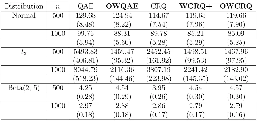
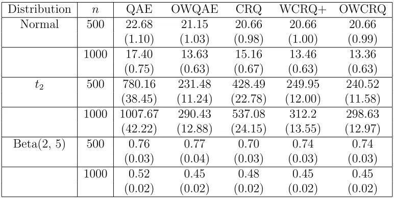
Tables 2.3 and 2.4 summarize the mean squared error (MSE) of different estimators of β in Examples 1 and 2, respectively. For Example 3, we report the mean integrated squared error (MISE) defined as
MISE = 1 500
500
X
j=1
{(βbj1−β1)2 + (βbj2−β2)2},
whereβbj1 and βbj2 are the estimators ofβ1 andβ2 from thejth simulation. Tables 2.3-2.5 suggest that, for all three types of distributions, OWCRQ and OWQAE have similar performance, which agrees with the asymptotic theory. For the heavy-tailed t2
distribu-tion, OWQAE and OWCRQ are more efficient than WCRQ+, which loses some efficiency due to the nonnegative weights constraint employed. In addition, for the t2 distribution,
the three methods involving weight estimation perform significantly better than the two methods QAE and CRQ based on equal weights. For normal errors, optimally weighted methods still have some efficiency gain over the equally weighted estimators but the gain is less obvious as that for thet2 distribution. For the short-tailed Beta(2, 5) distribution,
Table 2.3: The 103×MSE of different estimators of β in Example 1. The values in the
parentheses are the standard errors of 103×MSE.
Distribution n QAE OWQAE CRQ WCRQ+ OWCRQ
Normal 500 11.54 10.29 10.52 9.96 9.96
(0.76) (0.72) (0.74) (0.66) (0.66)
1000 8.82 7.16 7.78 7.19 7.17
(0.61) (0.51) (0.54) (0.52) (0.52)
t2 500 349.89 101.01 173.39 104.41 100.58
(20.08) (6.43) (11.01) (6.71) (6.40) 1000 628.92 148.91 302.17 167.87 159.20 (39.72) (8.78) (19.09) (10.22) (9.69)
Beta(2, 5) 500 0.39 0.39 0.37 0.39 0.40
(0.03) (0.03) (0.03) (0.02) (0.03)
1000 0.26 0.25 0.24 0.24 0.24
(0.01) (0.01) (0.01) (0.01) (0.01)
Table 2.4: The 103×MSE of different estimators of β in Example 2. The values in the
parentheses are the standard errors of 103×MSE.
Distribution n QAE OWQAE CRQ WCRQ+ OWCRQ
Normal 500 129.68 124.94 114.67 119.63 119.66
(8.48) (8.22) (7.54) (7.96) (7.90)
1000 99.75 88.31 89.78 85.21 85.09
(5.94) (5.60) (5.28) (5.29) (5.25)
t2 500 5493.83 1459.47 2452.45 1498.51 1467.96
(406.81) (95.32) (161.92) (99.53) (97.95) 1000 8044.79 2116.36 3807.19 2241.42 2182.90 (518.23) (144.46) (223.98) (145.35) (143.02)
Beta(2, 5) 500 4.25 4.54 3.95 4.54 4.57
(0.28) (0.29) (0.26) (0.30) (0.30)
1000 2.97 2.88 2.86 2.79 2.79
Table 2.5: The 103×MISE of different estimators in Example 3. The values in the paren-theses are the standard errors of 103×MISE.
Distribution n QAE OWQAE CRQ WCRQ+ OWCRQ
Normal 500 22.68 21.15 20.66 20.66 20.66
(1.10) (1.03) (0.98) (1.00) (0.99)
1000 17.40 13.63 15.16 13.46 13.36
(0.75) (0.63) (0.67) (0.63) (0.63)
t2 500 780.16 231.48 428.49 249.95 240.52
(38.45) (11.24) (22.78) (12.00) (11.58) 1000 1007.67 290.43 537.08 312.2 298.63 (42.22) (12.88) (24.15) (13.55) (12.97)
Beta(2, 5) 500 0.76 0.77 0.70 0.74 0.74
(0.03) (0.04) (0.03) (0.03) (0.03)
1000 0.52 0.45 0.48 0.45 0.45
(0.02) (0.02) (0.02) (0.02) (0.02)
2.4
Application to Chicago Precipitation Data
An important topic in climate studies is quantifying extremal phenomena such as heavy precipitation or high temperature, for which quantile regression serves as a promising tool. For illustration, we apply the proposed methods to the statistical downscaling of daily precipitations in the Aurora station of Chicago, IL. The responseY is the observed daily precipitation (inch) at the station from 1957 to 2002, and the covariate X is the simulated daily precipitation from the ERA-40 reanalysis model introduced in Uppala et al. (2005).
Since we are interested in estimating the extremely heavy precipitation conditioning on X, we only include the wet days data. In this data set 30% of the days are wet with yi >0. Since in climate studies it is commonly assumed that the percentage of wet days in the future is the same as in the past and prediction is based on the simulated daily precipitation, we define the wet days data as the pairs of (yi, xi) with xi exceeding its 70th sample percentile. This yields a data set of 4816 observations.
0.990 0.992 0.994 0.996 0.998
100
200
300
400
500
600
700
τ
β
^(τ
)
Figure 2.1: Local quantile regression estimates of the slope at upper quantiles for the precipitation data in Aurora station.
hypothesis H0 : β(0.990) = β(0.991) = . . . = β(0.995) and obtain a p-value=0.794.
However, the test for H0 : β(0.990) = . . . = β(0.996) = β(0.997) = β(0.998) yields
a p-value of 4−10, suggesting a possible violation of the common slope assumption for τ ≥ 0.996. Therefore, we choose five quantile levels 0.990,0.991, . . . ,0.995 to apply the proposed combined estimation methods.
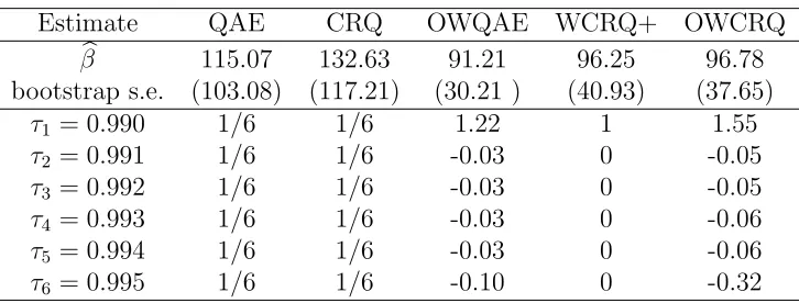
Table 2.6 summarizes the estimated slopes from different methods. The values in the parentheses are the bootstrap standard errors based on 1000 bootstrap samples obtained by sampling the paired observations (yi, xi) with replacement. It is noticed thatβbQAE and
b
βCRQ are larger than the other estimates, which is partially due to the fact that these two methods enforce equal weights at the six quantiles including the higher quantile τ = 0.994, at which the quantile slope estimation β(0.994) is the largest among the sixb slope estimations. In addition, the estimatorsβQAEb andβCRQb have larger variances, which lead to insignificance in the slope. In contrast, the OWQAE, OWCRQ and WCRQ+ estimators have smaller variances, and all three showed that at the high quantiles, the simulated daily precipitation has a significant positive effect on the observed precipitation and thus can serve as a good predictor for high precipitation.
Table 2.6: The upper part of the table summarizes the estimated common slope βb for the proposed methods and the bootstrap standard error (s.e.). The lower part of the table presents the quantile-specific weights given by different methods based on the estimated extreme value index ˆξ = 0.29.
Estimate QAE CRQ OWQAE WCRQ+ OWCRQ
b
β 115.07 132.63 91.21 96.25 96.78
bootstrap s.e. (103.08) (117.21) (30.21 ) (40.93) (37.65)
τ1 = 0.990 1/6 1/6 1.22 1 1.55
τ2 = 0.991 1/6 1/6 -0.03 0 -0.05
τ3 = 0.992 1/6 1/6 -0.03 0 -0.05
τ4 = 0.993 1/6 1/6 -0.03 0 -0.06
τ5 = 0.994 1/6 1/6 -0.03 0 -0.06
τ6 = 0.995 1/6 1/6 -0.10 0 -0.32
error (PE) is defined as:
P E =
2407
X
i=1
ρτ{yi−QbY(τ|xi)}, τ ∈ {0.990, . . . ,0.995},
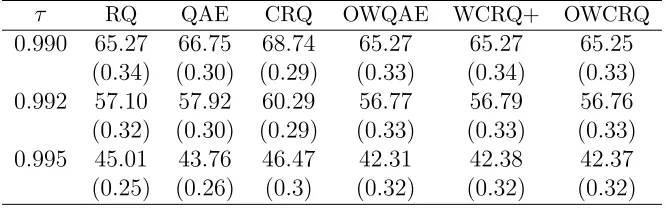
where{(yi, xi), i= 1, . . . ,2407}are in the validation set. The cross validation is repeated 500 times and the mean of PE is reported at quantile levels 0.990, 0.992 and 0.995 in Table 2.7. Results show that the proposed optimally weighted methods perform generally better than the equally-weighted methods QAE and CRQ and the local quantile regression method (RQ). Moreover, the gain in the prediction accuracy of the optimally weighted methods increases as the quantile level gets more extreme.
2.5
Proof
We first introduce some notations. Denote
an =
p
(1−τ)n F0−1(τ)−F0−1(eτm)
and ak =
p
lk(1−τ)n F0−1(τk)−F0−1(eτmk)
, (2.14)
Table 2.7: The prediction error of different methods at quantile levels 0.990, 0.992 and 0.995. The values in the parentheses are the standard errors.
τ RQ QAE CRQ OWQAE WCRQ+ OWCRQ
0.990 65.27 66.75 68.74 65.27 65.27 65.25 (0.34) (0.30) (0.29) (0.33) (0.34) (0.33) 0.992 57.10 57.92 60.29 56.77 56.79 56.76 (0.32) (0.30) (0.29) (0.33) (0.33) (0.33) 0.995 45.01 43.76 46.47 42.31 42.38 42.37 (0.25) (0.26) (0.3) (0.32) (0.32) (0.32)
Proof of Theorem 2.2.1. At the τkth quantile, the local quantile estimator of the coefficients in model (2.1) is defined as
(αbk,βbk) = argmin(α,β) n X
i=1
ρτk(yi−α−x
T i β).
Denote btn,k = ak(αbk−α0,k) and bzn,k = ak(βbk−β0), k = 1, . . . , K. By Theorem 5.1 of Chernozhukov (2005), we have
(btn,1,bzn,1, . . . ,btn,K,bz T n,K)
T d →N
0,
m−ξ−1 ξ
−2
e
Γ⊗ 1 0
0 D
!−1
,
where Γe is a K×K matrix with the (k, k0)th element as min(lk, lk0)/
√
lklk0. Therefore,
we have
an(bβW QAE−β0) = K X
k=1
$kan akb
zn,k d
→N 0, $TΦ−1(ξ)ΓΦ−1(ξ)$
m−ξ−1 ξ
−2
D−1
! .
Lemma 2.5.1 For a sequence of quantiles τ1, . . . , τK with τk →1 and (1−τk)n→ ∞, min(τk, τk0)−τkτk0
1−τ ∼min(lk, lk0),
Proof. Letτ∗ = 1−τ, τk∗ = 1−τk. Therefore, τk∗/τ
∗ →l
k, k = 1, . . . , K, and τ∗ →0. It’s easy to show that min(τk, τk0)−τkτk0 = min(τ∗
k, τ
∗
k0)−τk∗τk∗0.For any k, k0 = 1, . . . , K,
min(τk, τk0)−τkτk0
1−τ =
min(τk∗, τk∗0)−τk∗τk∗0
τ∗
= τ
∗[min(l
k, lk0) +o(1)−τ∗{lk+o(1)}{lk0+o(1)}]
τ∗
= min{lk, lk0 +o(1)} −τ∗{lk+o(1)}{lk0 +o(1)}
∼ min(lk, lk0).
Lemma 2.5.2 Under conditions A3-A5, ak/an →l ξ+1/2
k for any k = 1, . . . , K.
Proof.Since ∂F0−1(τ)/∂τ = 1/f0{F0−1(τ)}, A4 means that for any x >0
f0{F0−1(1−τ
∗)}
f0{F0−1(1−xτ∗)}
∼x−ξ−1, asτ∗ →0. (2.15)
For any δ >0, note thatdF0−1(1−sδ)/ds=−δf0{F0−1(1−sδ)}
−1
. Therefore, Z m
1
1
f0{F0−1(1−sδ)}
ds= F
−1
0 (1−δ)−F
−1
0 (1−mδ)
δ . (2.16)
Combining (2.15) and (2.16) gives F0−1(τk)−F0−1(eτmk)
lk(1−τ)/f0{F0−1(τk)}
∼ f0{F0−1(τk)}
F0−1{1−(1−τk)} −F0−1{1−m(1−τk)} 1−τk
= f0{F0−1(τk)} Z m
1
1
f0[F0−1{1−s(1−τk)}] ds
= Z m
1
f0[F0−1{1−(1−τk)}] f0[F0−1{1−s(1−τk)}]
ds
∼ Z m
1
s−ξ−1ds = m
−ξ−1
Therefore, applying (2.15) and (2.17), we have
ak an
= p
nlk(1−τ) p
n(1−τ)
F0−1(τ)−F0−1(eτm) F0−1(τk)−F0−1(eτmk)
= plk
F0−1(τ)−F0−1(τem) (1−τ)/f0{F0−1(τ)}
(1−τ)/f0[F0−1(τ)]
lk(1−τ)/f0{F0−1(τk)}
lk(1−τ)/f0{F0−1(τk)} F0−1(τk)−F0−1(eτmk)
∼ plk
m−ξ−1 −ξ
1 lk
lξk+1 −ξ m−ξ−1
=lξ+
1 2
k .
Proof of Theorem 2.2.2. For notational simplicity, we write bθW CRQ =
(αb1, . . . ,αbK,βb T
)T in this proof. Let b
un,k = ak(αbk − α0,k), k = 1, . . . , K, and ubn = an(bβ−β0), where (α0,1, . . . , α0,K,β0) are the true parameters. From (2.7), it is clear that
(bun,1, . . . ,ubn,K,ubn) is the minimizer of
Ln=
an p
n(1−τ) K X k=1 ωk n X i=1 ρτk
yi−xTi β0−α0,k− uk ak − xT i u an
−ρτk(yi−x
T
i β0−α0,k)
with respect to (u1, . . . , uk,u). Using Knight’s identity (Knight, 1998),
ρτ(u−v)−ρτ(u) = −v{τ−I(u <0)}+ Z v
0
{I(u≤s)−I(u≤0)}ds,
we can rewrite Ln asLn .
=Ln,1+Ln,2,where
Ln,1 =
an p
n(1−τ) K X k=1 ωk n X i=1 uk ak +x T i u an
{I(i,k <0)−τk},
Ln,2 =
an p
n(1−τ) K X k=1 ωk n X i=1 Z uk ak+
xTiu
an
0
{I(i,k 6s)−I(i,k 60)}ds,
and i,k =yi−xTi β0−α0,k. Denotingψi,k =I(i,k <0)−τk, we have
Ln,1 =
an p
n(1−τ) K X k=1 ωk ak n X i=1
ψi,kuk+
an p
n(1−τ) K X k=1 ωk an n X i=1
ψi,kxTi u
= K X
k=1
Wn,kuk+WTnu . =Wf
T
where
Wn,k = p ωk n(1−τ)
an ak
n X
i=1
ψi,k, Wn =
1 p
n(1−τ) K X k=1 n X i=1
ωkψi,kxi,
f
Wn= (Wn,1, . . . , Wn,K,WTn) T
, and Ue = (un,1, . . . , un,K,uTn) T
.
We next derive the limiting distribution of Wfn. Denote
Ti =
ω1
p
(1−τ) an a1
ψi,1, . . . ,
ωK p
(1−τ) an aK
ψi,K,STi !T
,
where Si = (1−τ)−1/2 PK
k=1ωkψi,kxi. Note that Ti are i.i.d. with mean 0 and co-variance matrix Vn. For k, k0 = 1, . . . , K, the (k, k0)th element of Vn is,
Vn(k, k0) = cov( ωk p
(1−τ) an ak
ψi,k, ωk0
p
(1−τ) an ak0
ψi,k0)
= ωkωk0 (1−τ)
a2
n akak0
{min(τk, τk0)−τkτk0}
→ ωkωk0l
−ξ−1 2
k l
−ξ−1 2
k0 min(lk, lk0), (2.19)
where Lemmas 2.5.1 and 2.5.2 are used to prove the last step. Under condition A2,
V ar(Si) = E{V ar(Si|xi)}+V ar{E(Si|xi)}
= E
(
xixTi K X
k=1
K X
k0=1
ωkωk0
min(τk, τk0)−τkτk0
1−τ
) + 0 = D K X k=1 K X
k0=1
ωkωk0
min(τk, τk0)−τkτk0
1−τ →Dω
TΓω.
In addition, for any k = 1, . . . , K,
cov p ωk (1−τ)
an ak
ψi,k,Si !
= ωk (1−τ)
an ak E ( ψi,k K X j=1
ωjψi,jxi !)
= ωk (1−τ)
an akE
(
E ψi,k K X
j=1
ωjψi,jxi xi !)
where the last step is due to the assumption that E(X) = 0. Combining (2.19)-(2.20) gives the limit of Vn
Vn →V =
V1 0
0 DωTΓω
!
, (2.21)
where V1 is a K×K matrix with the (k, k0)th element ωkωk0l
−ξ−1 2
k l
−ξ−1 2
k0 min(lklk0), and
k, k0 = 1, . . . , K. Applying the multivariate Central Limit Theorem and Slutsky theorem toTi, we can show that
f
Wn= 1 √ n
n X
i=1 Ti
d
→N(0,V). (2.22)
Now we consider the second part of the objective function Ln,Ln,2. By the definitions
of an and ak, we have
Ln,2 =
K X
k=1
ωk
F0−1(τk)−F0−1(eτmk) F0−1(τ)−F0−1(τem)
Gkn,
where
Gkn = p ak lk(1−τ)n
n X
i=1
Z uk
ak+
xTiu
an
0
{I(i,k 6s)−I(i,k 60)}ds
= n X
i=1
Z uk+akanxTiu
0
I(i,k 6 ask)−I(i,k 60) p
lk(1−τ)n
Furthermore, we have
E(Gkn) = nE "
Z uk+akanxTiu
0
Fi
Fi−1(τk) +s/ak −Fi{Fi−1(τk)} p
lk(1−τ)n
ds #
(iterated expectations)
(i)
= nE
Z uk+anakxTiu
0
fi[Fi−1(τk) +o{F0−1(τk)−F0−1(eτmk)}]s ak
p
lk(1−τ)n
ds !
(ii)
∼ nE
"
Z uk+akanxTiu
0
fi{Fi−1(τk)}s ak
p
lk(1−τ)n ds
#
= nE
" 1 2(uk+
ak an
xTi u)2 fi{F
−1
i (τk)} ak
p
lk(1−τ)n #
= E
1 2(uk+
ak an
xTi u)2 F
−1
0 (τk)−F0−1(eτmk) lk(1−τ)/fi{Fi−1(τk)}
(iii)
∼ E
1
2(uk+l ξ+12
k x T i u)
2
K(xi)−ξ
m−ξ−1 −ξ
. (2.23)
By Taylor expansion and the fact that (1−τ)n → ∞,
s/ak=s{F0−1(τk)−F0−1(eτmk)}/ p
lk(1−τ)n=o{F0−1(τk)−F0−1(τemk)},
then equation (i) in (2.23) is proven. The equation (ii) holds because
fi{Fi−1(τk) +o F0−1(τk)−F0−1(eτmk)
} ∼fi{Fi−1(τk)}
as τk → 1, which is derived following the same arguments as in the proof of Lemma 9.6 in Chernozhukov (2005). The equation (iii) is proven as follows. By condition A3, as τ →1,
fi
Fi−1(τ) =fU{α(τ)|xi} ∼f0
F0−1(τ) . Therefore,
F0−1(τk)−F0−1(eτmk) lk(1−τ)/fi{Fi−1(τk)} ∼
F0−1(τk)−F0−1(τemk) lk(1−τ)/f0{F0−1(τk)}
. (2.24)
Combining (2.24) and (2.17), we have
F0−1(τk)−F0−1(eτmk) lk(1−τ)/fi{Fi−1(τk)}
∼ m
−ξ−1
which together with Lemma 2.5.2 proves equation (iii). Furthermore, we can show that V ar(Gk
n) → 0 by following the same arguments as in the proof of Lemma 9.6 in Cher-nozhukov (2005). In Lemma 2.5.2 we showed that {F0−1(τ) − F0−1(eτm)}/{F0−1(τk) − F0−1(eτmk)} ∼lξk. Therefore, we have
Ln,2
p
→ E
( K X
k=1
ωkl
−ξ k
1
2(uk+l ξ+12
k x T i u)
2
m−ξ−1 −ξ
)
=
m−ξ−1 −ξ K X k=1 ωk 1 2u 2 kl −ξ k + 1 2l ξ+1 k u T Du . (2.26)
Combining (2.18), (2.22) and (2.26), we get
Ln d
→L∞≡
X
k=1
Wkuk+WTu+
m−ξ−1 −ξ K X k=1 ωk 1 2u 2 kl −ξ k + 1 2l ξ+1 k u TDu ,
where Wf = W1, . . . , WK,WT T
is a random vector following the distribution N(0,V) withV defined in (2.21). Since the objective functionL∞is quadratic inUe, the minimizer of L∞ is
uk,∞ =
m−ξ−1 ξ
ωkl
−ξ k
−1
Wk, fork = 1, . . . , K,
u∞ =
m−ξ−1 −ξ
−1
{φT(ξ)ω}−1D−1W,
where φ(ξ) = (l1ξ+1, . . . , lKξ+1)T. By the definition ofW, we have
u∞∼N 0,
ωTΓω
{φT(ξ)ω}2
m−ξ−1 −ξ
−2
D−1
! .
Note thatωk ≥0, k= 1, . . . , K, then the application of the convexity lemma in Pollard (1991) gives
an(bβW CRQ−β0) =ubn d →u∞.
The proof of the statements in Remark 2 relies on the following Lemma 2.5.3.
function.
Proof.We first prove (i). Note that
f0(x) = a
ξ+1−(ξ+ 1)axξ+ξxξ+1
(a−x)2 (2.27)
has the same sign as that of (a/x)ξ+1 −(ξ + 1)a/x+ξ. Consider the function s(t) =
tξ+1 −(ξ + 1)t +ξ, t > 0. For ξ > 0, s00(t) = ξ(ξ+ 1)tξ−1 > 0, so s(t) is a convex
function that achieves its minimum at t = 1. Since s(1) = 0, s(t) and f0(x) are both nonnegative. Thusf(x) is an increasing function for ξ >0. To prove (ii), we can use the same technique to show that s(t) is a concave function achieving its maximum att = 1, and thus f0(x)≤0 for all x >0.
Proof of Remark 2. Recall that the matrix Γ is a K ×K matrix with the (k, k0)th element defined as min(lk, lk0). Then it can be shown that Γ−1 is a band matrix with the
following form
Γ−1 = 1
l1−l2 −
1
l1−l2 0 0 0
− 1
l1−l2
1
l1−l2 +
1
l2−l3 −
1
l2−l3 0 0
0 − 1
l2−l3
1
l2−l3 +
1
l3−l4 0 0
0 0 − 1
l3−l4 . .. −
1
lK−2−lK−1 0
0 0 0 l 1
K−2−lK−1 +
1
lK−1−lK −
1
lK−1−lK
0 0 0 − 1
lK−1−lK
lK−1
LK(lK−1−lK)
.
Therefore, the optimal weights Γ−1φ(ξ)/1T KΓ
−1φ(ξ) = (ω
k)Kk=1, where
ω1 =c
lξ1+1 l1−l2
− l ξ+1 2
l1−l2
!
, ωK =c
lK−1
lK−1−lK
(lKξ −lξK−1)
,
and ωk =c l ξ+1
k −l ξ+1
k+1
lk−lk+1
−l ξ+1
k−1−l
ξ+1
k lk−1−lk
!
, fork = 2, . . . , K−1,
where c=1T KΓ
−1φ(ξ) is a positive constant. We consider the three different cases
sepa-rately.
(i) Case 1 (ξ >0). Note that l1 > l2 > . . . > lK. Obviously ω1 > 0,ωK <0. For any k = 2, . . . , K−1, letf(x) = l
ξ+1
k −xξ+1
2.5.3 .
(ii) Case 2 (ξ = 0). It is easy to show that ω1 = 1 andω2 =. . .=ωK = 0.
(iii) Case 3 (−1/2 < ξ <0). By Lemma 2.5.3 (ii) and the similar technique as used in the proof for case 1, we can show that ωk>0 fork = 1, . . . , K.
The proof of Proposition 2.2.1 relies on the following lemma.
Lemma 2.5.4 (Lemma 2 of Zhao and Xiao, 2013) Let S be a K ×K symmetric
positive-definite matrix and v be any non-zero K × 1 column vector. Define M =
vTS−1vS −vvT. Then (i) for any column vector z, zTM z ≥ 0; and (ii) zTM z = 0 holds if and only if z =cS−1v for some real constant c.
Proof of Proposition 2.2.1. Since the matrix Γ is positive-definite and symmetric, and φ(ξ) is non-zero, by Lemma 2.5.4 (i), we have
ωTφT(ξ)Γ−1φ(ξ)Γω−ωTφ(ξ)φT(ξ)ω ≥0, for anyω∈RK. (2.28)
Note thatφT(ξ)Γφ(ξ) is a scalar, (2.28) can be expressed as ωTΓω
ωTφ(ξ)φT(ξ)ω =σ
2
W CRQ(ω)≥ {φ T
(ξ)Γφ(ξ)}−1, for anyω ∈RK.
Lemma 2.5.4 (ii) then implies that the equality in (2.28) holds if and only ifω=cΓ−1φ(ξ) for some constant c.
Proof of Theorem 2.2.3. By the definitions, B(θ) is the first derivative of E{A(θ)}. With the Taylor series expansion, we get
E{A(eθ)}=E{A(θ0)}+B(¯θ)(eθ−θ0), (2.29)
where ¯θ lies between θ0 and eθ. Define
rn(δ) = A(θ+δ)−A(θ) =
K X
k=1
n X
i=1
ω(ko)zi,k
I{yi−zTi,k(θ+δ)<0} −I(yi−zTi,kθ<0)
Applying Lemma 4.1 of He and Shao (1996), we have the uniform approximation
sup
δ:||δ||≤C
||rn(δ)−E{rn(δ)}||=Op(√nlogn||δ||1/2), for some constantC.
Since eθ is an an-consistent estimator of θ0,
||{A(eθ)−A(θ0)} −[E{A(eθ)} −E{A(θ0)}]||=Op( √
nlogn||eθ−θo||1/2). (2.30)
Combining (2.29) and (2.30) gives
b
θOS−θ0 =−B(eθ)A(θ0)−Rn,
whereRn =B(eθ)−1{B(eθ)−B(¯θ)}(eθ−θ0) +B(eθ)−1Op( √
nlogn||eθ−θo||1/2).Following similar arguments as in the proof of Theorem 3 in Bradic et al. (2011), we can show that Rn is op(1/an). Consequently, to prove Theorem 2.2.3, we only need to consider an{B(eθ)A(θ0)}. Since θe is a consistent estimator, by Slusky theorem, it is sufficient to show the asymptotic normality of an{B(θ0)A(θ0)}. By the regularly varying property
in (2.25), Lemma 2.5.2 and the multivariate CLT, we can show that
an{B(θ0)A(θ0)}
d
→N 0,T−1J T−1 ,
where
T =
m−ξ−1 −ξ
ω(1o)l1ξ+1 0T
. .. ...
ωK(o)lξK+1 0T 0 . . . 0 ωToptφ(ξ)D
, J = J1 0
0 DωT
optΓωopt,
!
and J1 is a K ×K matrix with the (k, k0)th element ωkωk0min(lk, lk0). By some linear
algebra, we can show that the lower rightp×p block of T−1J T−1 is
ωT
optΓωopt
{φT(ξ)ωopt}2
m−ξ−1 −ξ
−2
D−1.
The proof is completed by plugging in ωopt =Γ−1φ(ξ)/{1TKΓ