Bayesian analysis of circular data using wrapped distributions

(1)

Bayesian Analysis of Circular Data Using Wrapped

Distributions

Palanikumar Ravindran† Roche Palo Alto, Palo Alto, USA.

Sujit K. Ghosh

North Carolina State University, Raleigh, USA.

Institute of Statistics Mimeo Series# 2564

Summary. Circular data arise in a number of different areas such as geological, meteoro-logical, biological and industrial sciences. Standard statistical techniques can not be used to model circular data due to the circular geometry of the sample space. One of the common methods to analyze circular data is known as thewrapping approach. This approach is based on a simple fact that a probability distribution on a circle can be obtained by wrapping a prob-ability distribution defined on the real line. A large class of probprob-ability distributions that are flexible to account for different features of circular data can be obtained by the aforementioned approach. However, the likelihood-based inference for wrapped distributions can be very com-plicated and computationally intensive. The EM algorithm to compute the MLE is feasible, but is computationally unsatisfactory. A data augmentation method using slice sampling is proposed to overcome such computational difficulties. The proposed method turns out to be flexible and computationally efficient to fit a wide class of wrapped distributions. In addition, a new model selection criteria for circular data is developed. Results from an extensive simulation study are presented to validate the performance of the proposed estimation method and the model selection criteria. Application to a real data set is also presented and parameter estimates are compared to those that are available in the literature.

Keywords: Bayesian inference; MCMC; Wrapped Cauchy; Wrapped Double Exponential; Wrapped Normal

†Address for correspondence: Palani Ravindran, Roche Palo Alto LLC, 3431 Hillview Ave, Palo Alto, CA 94304, USA.

(2)

2 P. Ravindran and S. K. Ghosh

1. Introduction

Circular data arise from a variety of sources in our daily lives, where we consider the circle to

be the sample space. Some common examples are the migration paths of birds and animals,

wind directions, ocean current directions and patients’ arrival times in an emergency ward

of a hospital. Many examples of circular data can be found in various scientiﬁc ﬁelds such

as earth sciences, meteorology, biology, physics, psychology and medicine. To motivate the

use of circular data, we present a brief description of couple of examples from these ﬁelds.

In the ﬁeld of Physics, before the discovery of isotopes,? proposed testing the hypothesis

that atomic weights are integers subject to error. He converted the fractional parts of the

atomic weights to angles. He regarded these angles as a random sample from a circular

distribution with mean zero and tested for uniformity. This study resulted into the famous

Von Mises distribution on the circle.

A very good source of circular data is in the ﬁeld of biology. Migration path of birds

and animals has been the subject of many studies. The objective of these studies is to

ascertain whether the direction of migration is uniform. An example of the migration of

turtles is given in Figure??. In this ﬁgure, we present the circular histogram plot of the

data collected by Dr. E. Gould from John Hopkins University School of Hygiene and ﬁrst

cited by ?. The data represents the directions taken by the sea turtles after laying their

eggs. The predominant direction is 64◦, which is the direction the turtles took to return to

the sea.

Standard statistical techniques cannot be used to analyze circular data. This is due to

the circular geometry of the sample space. For example, the sample mean of a data set on

the circle is not the usual sample mean. Lety1, y2, . . . , yn be independent observations on

the unit circle, such that 0≤yj <2π,j= 1,2, . . . , n. The mean direction ¯yis not given by

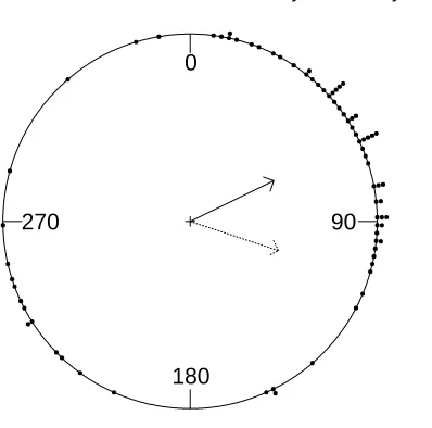
the usual deﬁnition, _n1n_j₌₁yj. This is illustrated in Figure??, where the dashed arrow is

the direction represented by _n1n_j₌₁y_j and the solid arrow represents the mean obtained

by vector addition. To ﬁnd the circular mean, we use vector addition techniques.

In general, the pth _{theoretical moment is deﬁned as} _E₍_eipY_{) =}_α

p+iβp, i=

√ −1, for

p= 1,2, . . .. The mean direction is given by µ = arctan(β1/α1) and the mean resultant

is deﬁned as ρ=α2₁+β₁2, so thatE(eiY_{) =} _ρeiµ_{. In most applications it is of interest}

(3)

0

180

270 90

Fig. 1. Circular histogram plot of the turtle data. Solid line indicates circular mean and dashed line indicates the linear mean.

generally provides a consistent estimate of the theoreticalpthmoment (See p.21?). However

such a nonparametric method cannot be easily generalized to regression problems using

link function viaµ. Typically parametric circular distribution are used to model the error

part of the regression models (See?, ch.11). Also no ﬁnite sample standard errors of the

sample moments are available. As a ﬁrst step towards regression models, we investigate the

performance of the estimation procedures for parametric models. Thus, in this article we

focus only on estimatingµandρfor a wide class of wrapped distributions.

In the literature several statistical approaches are available to model circular data. In

Section??, we use the wrapping method to generate a ﬂexible class of circular distributions.

In Section 3, we discuss classical and Bayesian methods to obtain estimates of the parameters

of wrapped circular distributions. As the Bayesian methods have the advantage of obtaining

a ﬁnite sample estimate of the variability (for example, the posterior standard deviation),

we use slice sampling as proposed in? within a data augmentation method for parameter

estimation. We propose to use two model selection criteria in Section 4. In Section 5, we

present results from extensive simulation studies to validate the frequentist performance of

the methods developed in Sections 3 and 4. In Section 6, we apply our method to a real

data set involving the movement of ants. Finally we conclude with some discussions on

(4)

2. Statistical Approaches to model circular data

Many methods and statistical techniques have been developed to analyze and understand

circular data. The popular approaches have been embedding, wrapping and intrinsic

ap-proaches. A good overview of the embedding and intrinsic approaches can be found in?

and?. We describe only the wrapping approach in this article.

2.1. The Wrapping Approach

In the wrapping approach, given a known distribution on the real line, we wrap it around

the circumference of a circle with unit radius. Technically this means that ifU is a random

variable on the real line, then the corresponding random variableY on the circle is given

byY =U(mod 2π). Equivalently, the wrapped version ofU is obtained by deﬁning

Y =U−2π₂U_π, (1)

where [u] = largest integer ≤ u. Let the distribution function of U on the real line be

denoted byF. Then the distribution function ofY denoted byFw can be obtained as,

Fw(y) = Pr(Y ≤y) =

∞

k=−∞

[F(y+ 2πk)−F(2πk)].

This implies that if the densityf ofU exists, then the wrapped densityf_w is given by,

f_w(y) =

∞

k=−∞

f(y+ 2πk), 0≤y <2π. (2)

An excellent overview of the properties of the wrapped distributions can be found in?. In

most cases the above series can not be written in closed form except in few cases such as

Cauchy distribution. The density of the wrapped Cauchy (WC) distribution is given by

fW C(y) = _πσ1

∞

k=−∞

1 +

y+2πk−µ σ

2 −2

, 0≤y <2π, (3)

whereµ is the location parameter andσis the scale parameter. Using inversion theorem,

(??) can be simpliﬁed to

f_{W C}(y) =₂1_π₁₊_ρ2₋12−ρρcos(2 y−µ),

where ρ = e−σ_{. We consider two other wrapped distributions, for which no closed form}

(5)

by,

fW N(y) = _σ√1₂_π

∞

k=−∞

e−(y+2πk−µ)2/(2σ2), 0≤y <2π. (4)

Another popular wrapped distribution, known as the wrapped double exponential (WDE)

is described by it density,

f_{W DE}(y) = ₂1_σ

∞

k=−∞

e−|y+2πk−µ|/σ, 0≤y <2π. (5)

In Section??, we describe a Monte Carlo method based on slice sampling to obtain estimate

ofµandρunder (??), (??) and (??).

It follows that, a rich class of distributions on the circle can be obtained using the

wrapping technique, as we can wrap any known distribution on the real line to the circle.

The main diﬃculty in working with this approach has been that in most cases, the form

of the densities and distribution functions are large sums (e.g. (??) and (??)) and can

not be simpliﬁed as closed forms except for few cases (e.g. (??)). Due to this complexity,

maximum likelihood techniques for point estimation and hypothesis testing can not be

easily implemented. The main contribution of this paper is to present a general approach

to obtain parameter estimates for a wide class of wrapped distributions. This can be

achieved as follows. For a given probability distribution on the circle, we make assumptions

that the original circular distribution was distributed on a line and was wrapped to a circle.

Therefore if we canunwrapthe distribution on the circle and obtain a distribution on the

real line, we can use all the standard statistical techniques for data on a real line. We

propose to perform this using the data augmentation approach. We use Bayesian methods,

so that we can easily obtain parameter uncertainty estimates based on the ﬁnite sample.

3. Parameter Estimation of Wrapped Distributions

It was shown by ? that the maximum likelihood estimate for wrapped Cauchy exists and

is unique for samples of size greater than two. They also gave a simple iterative algorithm

which would always converge to the maximum likelihood estimate (MLE). Calculating the

MLE for the wrapped Cauchy is possible because the density has a closed form

representa-tion. In general, wrapped distributions do not have closed form densities and consequently,

(6)

A diﬀerent approach for ﬁtting wrapped distributions was given by ? who used the

Expectation Maximization (EM) algorithm techniques to obtain parameter estimates from

the Wrapped Normal distribution. However, the E-step involves ratio of large inﬁnite sums,

which needs to be approximated at each step. This makes the algorithm computationally

ineﬃcient. In addition, the standard errors of the MLEs have to be evaluated based on

large-sample theory. We propose an alternative method that is more computationally eﬃcient

and ﬂexible to entertain a large class of wrapped distributions. Also, as a by-product, we

acquire ﬁnite sample interval estimates of the parameters of the wrapped distributions. This

is done using the data augmentation approach described in the following section.

3.1. The Data Augmentation Approach

The data augmentation approach was originally proposed by?. Extensions of this technique

can be found in the works of?,? and? and references therein. In the context of circular

data,? used it to study Von Mises distribution. ? used it to study the Wrapped Bivariate

Normal distribution and wrapped autoregressive process. We present a generic approach

based on slice sampling (see Neal, 2003) that can be used for a broad class of wrapped

distributions.

The main idea behind the data augmentation approach is to augment the original data

with some “additional data” that would simplify the original likelihood to a form that is

much easier to handle. In case of circular data, asY =U(mod 2π), the random variableU

on the real line, can be represented asU =Y + 2πK, whereY is the observed data on the

circle, andKis the number of timesU was wrapped to obtainY. Therefore, in this case if

we were able to “add” the information onK, and thusunwrapY, then we could observeU.

However, given Y, as the value of K is not unique, we obtain the conditional probability

distribution ofK givenY. To illustrate the unwrapping method, let us consider a location

scale family _σ1f(y−_σµ) on the real line. Then the corresponding wrapped density is obtained

from (??) as,

fw(y|µ, σ) =

∞

k=−∞

1

σf(

y+2πk−µ

σ ) (6)

In the above equation, we follow the convention that the location parameterµ=µ0(mod2π),

whereµ0 is the location parameter on the real line. In order to specify the full probability

(7)

direction, ρ (as deﬁned in Section 1) can be expressed as a function of σ. In general, we

will writeρ=h(σ), e.g. for wrapped normal familyρ=e−σ2/2_{, for wrapped Cauchy family}

ρ=e−σ _{and for wrapped double exponential family} _ρ₌ 1

1+σ2. Notice that by deﬁnition,

0< ρ <1.A class of non-informative prior for (µ, ρ) can be speciﬁed by a joint density of

(µ, ρ) as,

[µ, ρ] ∝ I_µ(0,2π)ρaρ−1(1−ρ)aρ−1,a_ρ>0, (7)

where Ix(A) denotes the indicator function, i.e., Ix(A) = 1 if x ∈ A and Ix(A) = 0,

otherwise. Viewing the wrapped numberKto be a random variable, from (??) we see that

the conditional density ofY givenK=kand the parametersµ, ρ is given by

fw(y|k, µ, σ) =

1

σ f(y

+2πk−µ

σ )Iy(0,2π) F(2π(k+1)_σ −µ)−F(2πk_σ−µ)

which is a truncated density of a location-scale family. It also follows that the marginal

density ofK given the parameters (µ, σ) can be obtained as,

Pr(K=k|µ, σ) = F(2π(k+1)_σ −µ)−F(2πk_σ−µ), k=. . . ,−1,0,1, . . .

Thus, we obtain a Bayesian hierarchical model by specifying the distribution ofygiven

k, µ, σ, then the conditional distribution of k given µ, σ and ﬁnally the prior distribution

for (µ, σ).

Given a random sample on the circle, y={y1, y2, y3, . . . , yn},0 ≤yj <2π, j = 1. . . n,

we unwrap the data by obtaining samples from the conditional distribution ofkgivenµ,σ

and the observed datay, where k={k1, k2, k3, . . . , kn}. This is will be referred to as the

data augmentation step. Then conditional on the augmented datay,k, we obtain samples

from the joint posterior distribution of (µ, σ) to complete the Gibbs cycle of the MCMC

method. From these samples, we obtain the marginal posterior distribution of µ and σ

given the observed datay, using the Ergodic Theorem of Markov Chain.

We provide a generic method to implement the MCMC method for a general class of

lo-cation scale family, whose density function is invertible. A functiony=f(x) is invertible if

f can be analytically or numerically inverted, or iff can be factorized into functions, which

can be analytically or numerically inverted. That is, we assume thatf(x) =T_t₌₁f_t(x) and

{f_t−1(y) : j = 1. . . T} are explicitly known functions or functions that can be computed

(8)

f(x) = e−x_e−e−x _{does not have an explicitly known inverse, but}_e−x _and_e−e−x _have

ex-plicitly known inverses. Alternatively, it is also possible to compute the inverse ofe−x_e−e−x

using numerical methods such as bisection method. But for our proposed algorithm we

re-strict ourselves to the former method. It is assumed thatρ=h(σ) is a monotone decreasing

function ofσand can be inverted. This is a reasonable assumption because in general, as

σ↓0,ρ↑1 and as σ↑ ∞, ρ↓0. These assumptions are satisﬁed for most wrapped

distri-butions including Wrapped Normal (WN), Wrapped Cauchy (WC) and Wrapped Double

Exponential (WDE) distributions. The general method will work even if ρ=h(σ) is not

a monotone decreasing function ofσ. These wrapped distributions are all symmetric and

unimodal. However, this method is not restricted only to these distributions.

In order to specify the required conditional distributions, we use the notation [θ1, . . . , θn]

to represent the joint density ofθ1, θ2, . . . , θnand [θ1|θ2, . . . , θn] to represent the conditional

density of θ1 given θ2, . . . , θn. By the term full conditional density of θ1, we mean the

conditional density ofθ1, given rest of the parameters.

The general method is as follows. The joint prior density of (µ, σ) is given by

[µ, σ] ∝ I_µ(0,2π)h(σ)aρ−1(1−h(σ))aρ−1|h(σ)|, a_ρ>0, ρ=h(σ)

For each observed direction yj, we augment a random wrapping number kj. The joint

density ofy,k, µandσis given by,

[y,k, µ, σ] ∝ y|k, µ, σ2 k|µ, σ2 µ, σ2

∝ 1

σn+n0

n

j=1

f(yj−µ+2πkj

σ )h(σ)aρ−

1+n1₍₁₋_h₍_σ₎₎aρ−1_h₁₍_σ₎_I

µ(0,2π),

where |h(σ)| can be factorized as _σ1n₀h(σ)n1h1(σ). The full conditional densities of k, µ

and σ are nonstandard densities. So we introduce auxiliary variables z and v. Let z =

{z0, z1, z2, z3}andv={v1, v2, v3, . . . , vn}, such that

[y,k, µ, σ] ∝

[y,k, µ,z,v, σ]dzdv

The joint density ofy,k, µ,z,v andσis given by,

[y,k, µ,z,v, σ] ∝ Iz0

0,_σn1+n0

n j=1

Ivj

0, f(yj−µ_σ+2πkj)

Iz1

0, h(σ)aρ−1+n1

Iz3(0, h1(σ))Iµ(0,2π)

Iz2

0,(1−h(σ))aρ−1I(aρ= 1) +I(aρ= 1)

(9)

It follows from the above equation that all the full conditional densities are standard

distributions that can be easily sampled using subroutines available in SAS, Splus, R and

other statistical softwares. In particular, as an illustration, we provide the standard full

conditionals that are needed to ﬁt a WDE model in the Appendix. The standard full

conditional densities that are needed to ﬁt other distributions can be found in the thesis of

the ﬁrst author.

4. Model selection

We now have a large class of parametric models that can be ﬁtted to a given circular data.

In order to select the best ﬁtting model, we use Deviance Information Criteria proposed by

? and a predictive loss approach developed by ?.

Deviance Information Criteria (DIC) is deﬁned as

DIC = 2E(Dev(µ, σ)|y)−Dev(E(µ, σ|y))

Deviance (?) is deﬁned as twice the negative of the log-likelihood. For example, for any

wrapped location-scale density,f_w() the deviance (Dev) is given by,

Dev(µ, σ) = −2log(

n

i=1

fw(yi))

= −2

n i=1 log( ∞

k=−∞ 1

σf(

yi+2πk−µ σ ))

≈ −2

n i=1 log( L

k=−L

1

σf(

yi+2πk−µ σ )),

whereLis a very large positive number. Given a set of models, the model with the lowest

DIC is chosen as the “best” model. For justiﬁcations on the use of DIC as a model selection

criteria see?.

Next, we use the decision theoretic framework of ? to deﬁne a model selection criteria

based on minimizing a predictive loss. For circular data the usual loss functions on the real

line are not well deﬁned. We propose a Circular Predictive Discrepancy (CPD) measure

based on posterior predictive distribution. Deﬁne yobs = (y1, ..., yn) as the observed data

and ypred = (y1pred, ..., ypredn ) as the predictive data obtained from the following posterior

predictive distribution,

(10)

where p(ypred_|_{µ, ρ}_{) denotes the sampling distribution of the data, which is the wrapped}

density evaluated atypred _given_µ_and _ρ_. _p₍_{µ, ρ}_|_yobs_{) denotes the posterior distribution of}

the parameters (µ, ρ) given the observed data yobs_{. In order to measure the discrepancy}

between observed and predicted quantities we use the following loss function and call it an

Absolute Predicted Errors (APE) deﬁned as,

AP E =

n

i=1

minypred_i −yi,2π−yipred−yi

.

Based on the above loss function we deﬁne the CPD as,

CP D = E[AP E|yobs]

Note that as in the case of linear loss functions, we can not break up the CPD into two

terms involving a goodness-of-ﬁt term and a penalty term. It is apparent that given a set

of models, we will prefer a model with the lowest CPD.

We use both of the above model selection methods to choose from a given set of wrapped

distributions. In order to see the performance of these model selection methods, we conduct

a simulation study and monitor the percentage of success. Details of such a simulation study

is presented in the next section.

5. Simulation studies

In this Section, we present couple of simulation studies to illustrate (i) the performance

of the parameter estimation method presented in Section 3 and (ii) the performance of

model selection criteria presented in Section 4. It is to be noted that we present only some

selected results of a much broader simulation study which can be found in the doctoral

thesis of the ﬁrst author. In terms of parameter estimation, we found that when data are

generated from the true model that is being ﬁtted, the parameter estimates obtained by the

data augmentation method (presented in Section 3) have very good frequentist properties

in terms of low bias and nominal standard errors. Also based on 95% posterior intervals,

we found that the coverage of such interval estimates are very close to the nominal level.

These results have been excluded in this article. However, we present results from the study

when the true model is misspeciﬁed. In order to study the sensitivity of the likelihood we

(11)

Von Mises distribution, we use the algorithm given by Best and Fisher (1978). For our

simulations we ﬁxedµ=π/21.5708 andρ= 0.5. We generatedn= 50 observations from

theV M(π/2,0.5) and then ﬁtted wrapped normal, wrapped Cauchy and wrapped double

exponential distribution to each of the data generated from the above mentioned Von Mises

distribution. We repeated the method 500 times to see the frequentist performance of the

Bayes method. In addition, to observe model selection issues, we computed model selection

criteria DIC and CPD to select the best model. In Table??, the percentages each of the

ﬁtted model chosen by the model selection criteria CPD and DIC are given. For model

ﬁtting, we useda_ρ = 0.5 for all priors. In our study (not shown here) we did not ﬁnd the

posterior summary to be very sensitive to the choice ofa_ρ, provideda_ρ∈(0,2].

We computed the posterior mean, standard deviation (s.d), 2.5 percentile, median and

97.5 percentile forµandρfor each simulation. The percentiles are computed with 0 radians

as the reference point on the circle. Usually, the reference point on the circle is chosen

diametrically opposite to the sample mean, or where the samples are sparsely distributed.

Note that, changing the reference point does not aﬀect the circular mean. The simulation

standard errors for each of these summary values are also computed. We also compute

the coverage probability (c.p) for the 95% posterior interval given by the 2.5th and 97.5th

percentile of the posterior distribution. After some preliminary studies, for all simulations,

we choose the burn-in period to be 2000 samples (i.e. throw away ﬁrst 2000 samples from

the MCMC chain) and then keep 5000 samples after burn in, to obtain posterior summary

values. All of these summary values are based on these ﬁnal 5000 samples. In Table??, we

present the empirical mean of the posterior summary values along with the standard error

(s.e.) of the posterior summary values. Notice that the empirical s.e.’s match well with the

estimated one given by the standard deviation of the posterior distribution. For instance,

the average posterior standard deviation ofµ under a WN model is 0.22, which matches

well with the Monte Carlo standard error of 0.21. Also the empirical coverage probability

for the estimation ofµusing a WN model is exactly same as the nominal level. However,

the results may not be that close for other models. For example, under a WDE model, the

empirical coverage probability is about 92% forµwhereas it is about 94% forρ. In general,

we see that the location parameterµis well estimated compared to the scale parameter ρ

even under model misspeciﬁcation. One of the beneﬁts of using a Bayesian method which

(12)

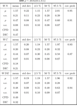
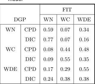
Table 1. Fitting WN, WC and WDE to VM(1.57, 0.5) distribution withρ∼Beta(0.5,0.5)

W N mean std dev 2.5 % 50 % 97.5 % cov prob µ 1.57 0.22 1.15 1.57 2.01 0.95 s.e. 0.21 0.11 0.23 0.20 0.39

ρ 0.47 0.08 0.31 0.47 0.60 0.91 s.e. 0.08 0.01 0.10 0.08 0.07

CPD 0.33

DIC 0.47

W C mean std dev 2.5 % 50 % 97.5 % cov prob µ 1.57 0.20 1.18 1.57 1.97 0.93 s.e. 0.20 0.08 0.23 0.20 0.32

ρ 0.44 0.07 0.30 0.45 0.58 0.87 s.e. 0.07 0.01 0.09 0.08 0.07

CPD 0.18

DIC 0.21

W DE mean std dev 2.5 % 50 % 97.5 % cov prob µ 1.57 0.19 1.19 1.57 1.96 0.92 s.e. 0.20 0.07 0.23 0.20 0.28

ρ 0.48 0.08 0.31 0.48 0.63 0.94 s.e. 0.08 0.01 0.10 0.09 0.07

CPD 0.49

(13)

Table 2. Performance of CPD and DIC in selecting the best model

FIT

DGP WN WC WDE

WN CPD 0.59 0.07 0.34

DIC 0.77 0.07 0.16

WC CPD 0.08 0.44 0.48

DIC 0.09 0.55 0.35

WDE CPD 0.17 0.29 0.55

DIC 0.24 0.38 0.38

performance of the estimates are quite good even from frequentist perspective. However,

it is noted that the proposed Bayesian method is computationally more intensive than the

comparable frequentist procedures. In SAS, on a Sparc 20 machine, on an average it took

about 50 minutes to perform the entire simulation for a given wrapped distribution.

In Table ??, we see that WN and WDE are performing well in estimating µ and ρ

when they come from a Von Mises distribution. It is expected that WN will perform

well because WN closely approximates the Von Mises distribution. WC model does not

perform well in estimating the mean resultant length. The lower than nominal coverage

probability of ρ indicates that WC is not robust in estimating the mean resultant length

of the distribution when the distribution is misspeciﬁed. However, the location parameter

is generally estimated very well. Using CPD, we ﬁnd that the WDE model gets picked up

most of the time (49%) as the best ﬁt to VM data. On the other hand, DIC picks WN more

often (47%) as the best ﬁt to VM data.

In order to study the performance of the model selection criteria presented in Section

4, we generated data from Normal, Cauchy and Double Exponential distributions on the

real line and wrapped them onto the circle (0, 2π). For our simulations, we ﬁxedµ=π/2

andρ= 0.5. We generatedn= 50 observations from theW N(π/2,0.5),W C(π/2,0.5) and

W DE(π/2,0.5). We then ﬁtted Wrapped Normal, Wrapped Cauchy and Wrapped Double

Exponential distributions to each of the three datasets. We repeated the method 500 times

to see the frequentist performance of model selection methods. For model ﬁtting we used

(14)

270

90

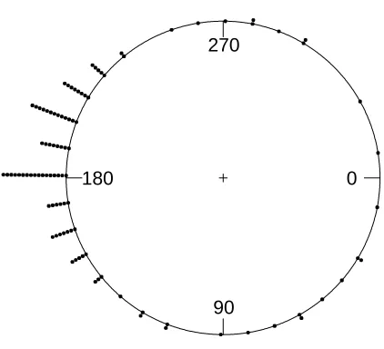
180 0

Fig. 2. Circular plot of the Jander’s Ant data

WN, WC and WDE. For each of the three DGP, we ﬁt WN, WC and WDE and report

the percentages, each of the ﬁtted model chosen by the model selection criteria DIC and

CPD. Notice that each row sums to unity. For instance, when we generate data from a

WN distribution and ﬁt all three distributions, CPD picks up WN as the best model 59%

of the time as compared to picking up 7% and remaining 34% by WC and WDE as the

best model, respectively. On the other hand DIC in this case performs much better in the

sense that it picks up WN as the best model 77% of the time. But the performance of

DIC is not uniformly better than CPD, for instance when data are generated from WDE,

CPD picks up the true model more often than the DIC. It appears that both CPD and DIC

are performing reasonably well in picking the correct distribution, though more separation

of the models are required for better performance. Notice that we used the same µ and

ρ parameter values for each of the three distributions. Aside for the performance of the

model selection criteria, another feature to observe is that, in general WDE model ﬁts well

even when the data is generated from other distributions like WN and WC. In this sense,

we conclude that the estimation ofµandρbased on a WDE model will be robust against

(15)

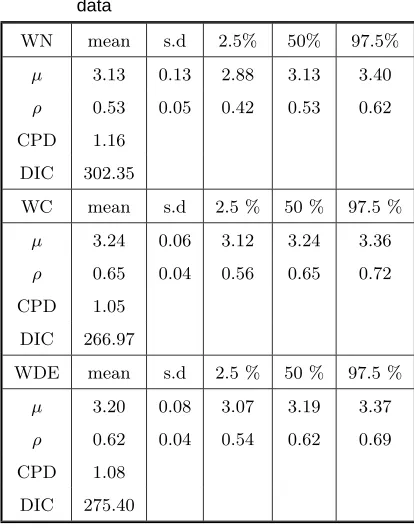
Table 3. Posterior summary val-ues of(µ, ρ)based on fitting WN, WC and WDE models to the Ant data

WN mean s.d 2.5% 50% 97.5% µ 3.13 0.13 2.88 3.13 3.40 ρ 0.53 0.05 0.42 0.53 0.62 CPD 1.16

DIC 302.35

WC mean s.d 2.5 % 50 % 97.5 % µ 3.24 0.06 3.12 3.24 3.36 ρ 0.65 0.04 0.56 0.65 0.72 CPD 1.05

DIC 266.97

WDE mean s.d 2.5 % 50 % 97.5 % µ 3.20 0.08 3.07 3.19 3.37 ρ 0.62 0.04 0.54 0.62 0.69 CPD 1.08

DIC 275.40

6. Application to real data sets

We analyze a data set that presents the orientation of the ants towards a black target

when released in a round arena. This experiment was originally conducted by? and later

mentioned in?. The data consists of 100 observations. For this data set, circular sample

mean and resultant direction are 3.20 radians (183◦) and 0.61 respectively.

We plot a circular histogram of this data in Figure ??. We ﬁt WN, WC and WDE

distributions to this data. We compute the posterior mean, standard deviation (s.d), 2.5

percentile, median and 97.5 percentile forµandρ. We have used a class of non-informative

priors for (µ, ρ) which is given in equation (??), but present the results only foraρ = 0.5,

in Table??.

While ﬁtting the data, initially we rejected the ﬁrst 2000 samples (burn-in period) of

the MCMC chain and kept the next 5000 samples after burn-in to do posterior inference.

(16)

10000 15000 20000 25000 30000 35000 40000

3.0

3.1

3.2

3.3

3.4

Iterations

Trace of mu

3.0 3.1 3.2 3.3 3.4

0123456

N = 30000 Bandwidth = 0.0082

Density of mu

10000 15000 20000 25000 30000 35000 40000

0.50

0.55

0.60

0.65

0.70

0.75

Iterations

Trace of rho

0.50 0.55 0.60 0.65 0.70 0.75

02468

N = 30000 Bandwidth = 0.005484

Density of rho

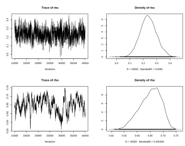
Fig. 3. MCMC output for parameters while fitting Wrapped Cauchy to ant data

burn-in time to 10000 samples and kept the next 30000 samples. We used multiple starting

values forµ and ρ, viz. µ = 3.2 and 0 andρ = 0.61 and 0.99. We ﬁnd that after 3000

samples, the two chains overlap each other and achieves good mixing. Carefully monitoring

other diagnostics aspects of convergence, such as auto/cross correlations using CODA (not

presented here), we assert that there was no apparent problem with MCMC convergence.

Summary values of the parameters are given in Table??.

To compare the models we use CPD and DIC. A smaller value of the model selection

criteria indicates a better ﬁt. From Table ??, we see that WC is performing best based

on CPD and DIC. WDE estimates are close to WC estimates. But the estimates from

WN are diﬀerent from WC and WDE. Using CODA, we obtained the trace plots and the

kernel density estimates of the parametersµ and ρbased on the wrapped Cauchy (WC)

distribution, which are presented in Figure??.

(17)

that WN does not ﬁt this data very well, which concurs with our ﬁnding as well. They

recommend a family of symmetric wrapped stable distributions (SWS, see?, p. 52) or a

mixture of SWS and circular uniform density for this data. Notice that WC belongs to

the SWS family and hence this conclusion agrees with the result obtained from the CPD

and DIC values. The test presented by? is based on a large-sample theory, whereas our

ﬁndings are based ﬁnite sample method.

7. Discussion

In this article, we provided a generic method to ﬁt a wide class of continuous wrapped

densities on the circle using MCMC methodology. We showed that using this method, we

can easily obtain samples from the joint posterior distribution, and hence, compute the

posterior summary values such as the posterior mean, standard deviation, 2.5 percentile,

median and 97.5 percentile for µ and ρ. From simulation-based studies, we found that

parameter estimates based on WDE are robust to erroneous models. In addition, we found

that the posterior distribution is not sensitive to the class of non-informative priors that we

proposed. We also studied the performance of two model selection criteria viz., CPD and

DIC, and using simulation studies we showed that both criteria perform well in selecting

the correct model from a set of given models. As an extension to this work, we have

developed regression models based on wrapped distributions and will be reported elsewhere.

Another extension is to consider correlated circular observations such as time series model

by wrapping autoregressive model on the line to a circle.

Acknowledgments

The authors would like to thank Dr. Kaushik Ghosh at the George Washington University,

for providing the Splus code to plot the circular histograms.

References

Best, D. J. & Fisher, N. I. (1978) Eﬃcient simulation of the Von Mises distribution.

(18)

Coles, S. (1998) Inference for circular distributions and processes.Statistics and Computing,

8, 105-113.

Damien, P., Wakeﬁeld, J. & Walker, S. (1999) Gibbs sampling for Bayesian non-conjugate

hierarchical models by using auxiliary variables.J. R. Statist. Soc. B,61, 331-344.

Damien, P. & Walker, S. (1999) A full Bayesian analysis of circular data using von Mises

distribution.The Canadian Journal of Statistics,27, 291-298.

Fisher, N. I. (1993)Statistical analysis of circular data., Cambridge Univ. Press, Cambridge.

Fisher, N. I. & Lee, A.J. (1994) Time series analysis of circular data.J. R. Statist. Soc. B,

56, 327-339.

Gelfand, A. E. & Ghosh, S. K. (1998) Model choice: A minimum posterior predictive loss

function.Biometrika,85, 1-11.

Higdon, D. M. (1998) Auxiliary variable methods for Markov Chain Monte Carlo with

applications.J. Am. Statist. Assoc.,93, 585-595.

Jander, R. (1957) Die optische Richtungsorientierung der roten Waldameise (Formica rufa

L.).Zeitschrift Fur Vergleichende Physiologie, 40, 162-238.

Kent, J. T. & Tyler, D. E. (1988) Maximum likelihood estimation for the wrapped Cauchy

distribution.Journal of Applied Statistics,15, 247-254.

Mardia, K. V. (1972)Statistics of directional data., Academic Press, London.

Mardia, K. V. & Jupp, P. E. (1999)Directional statistics., Wiley, Chichester.

McCullagh, P. & Nelder, J. A. (1989) Generalized Linear Models, 2nd ed., Chapman and

Hall, New York.

Neal, R.(2003) Slice sampling (with discussion).Annals of Statistics,31, 705-767.

Sengupta, A & Pal, C (2001) On optimal tests for isotropy against the symmetric wrapped

stable-circular uniform mixture family.Journal of Applied Statistics, 28, 129-143.

Spiegelhalter, D. J., Best, N. G., Carlin, B. P., & van der Linde, A. (2002) Bayesian

measures of model complexity and ﬁt, (with discussion and rejoinder). Journal of the

(19)

Stephens, M. A. (1969)Techniques for directional data.Technical Report 150, Department

of Statistics, Stanford University.

Tanner, M. A. & Wong W. H. (1987) The calculation of posterior distributions by data

augmentation.J. Am. Statist. Assoc.,82, 528-540.

van Dyk, D. A. & Meng, X. L. (2001) The art of data augmentation.Journal of

Computa-tional and Graphical Statistics,10, 1-50.

Von Mises, R. (1918) ¨Uber die “Ganzzahligkeit” der Atomgewicht und verwandte Fragen.

(20)

Appendix: Full conditional densities for the WDE model

The full conditional densities ofk,v,z,µandσ2 are given by

[kj|y,k−j, µ,z,v, σ] ∝ Ivj

0, e−|yj−µ

+2πkj| σ

,

⇒kj|y,k−j, µ,z,v, σ ∼ DU21π(µ−yj+σlogvj)

,₂1_π(µ−yj−σlogvj)

,

whereDU stands for Discrete Uniform.

vj|y,k, µ,z,v−j, σ ∼ U

0, e−|

yj−µ+2πkj|

σ ,

z0|y,k, µ,z−0,v, σ ∼ U0,_σn−21aρ+1

,

z1|y,k, µ,z₋₁,v, σ ∼ U

0,₍₁₊_σ1₂₎2aρ

,

µ|y,k,z,v, σ ∼ U[m_µ, M_µ],

wheremµ =

n

max

j=1 [yj+ 2πkj+σlogvj]

0 and

Mµ = n

min

j=1[yj+ 2πkj−σlogvj]

(2π).

σ|y,k, µ,z,v ∼ U[mσ, Mσ],

wherem_σ = maxn

j=1

|yj−µ+2πkj| −logvj

and

M_σ = 1

z

1

n−2aρ+1

0 1−z

1 2aρ

1

z

1 2aρ

1

,