The Use Of Hybrid Technique: Thresholding And Edge Detection For Identifying River From Aerial Photo

(1)

Jurnal Teknologi, 41(B) Dis. 2004: 1–20 © Universiti Teknologi Malaysia

THE USE OF HYBRID TECHNIQUE: THRESHOLDING AND EDGE DETECTION FOR IDENTIFYING RIVER

FROM AERIAL PHOTO

MOHD SHAFRY MOHD RAHIM1, NIK ISROZAIDI NIK ISMAIL2 & MOHD AZUAN SHAH IDRIS3

Abstract. The field of image processing is a broad field with many applications in science and industry. Image processing is used to manipulate and enhance an image, which ease the next process. This research involves the use of a hybrid techniques, which is a combination of thresholding and Sobel edge detection technique, to recognize a river from a grey scale image. Thresholding technique is used to reduce non-maxima pixels, weak edges and noise, whilst the edge detection technique is used to detect location of the edges. The output from this hybrid technique is compared to the existing techniques such as Sobel, Prewitt, Laplacian, and Robert Cross technique.

Keywords: Image processing, feature extraction, edge detection, aerial photo

Abstrak. Bidang pemprosesan imej merupakan satu bidang yang luas dengan pelbagai aplikasi terutama dalam bidang sains dan industri. Pemprosesan imej digunakan dalam manipulasi dan penambahbaikan imej untuk memudahkan proses seterusnya. Penyelidikan ini melibatkan penggunaan teknik hybrid yang menggabungkan teknik threshold dan teknik pengesanan sisi Sobel, untuk mengenal pasti sungai dari pada imej berskala kelabu. Teknik thresholding digunakan untuk mengurangkan piksel sisi yang tak maksima, piksel sisi yang lemah dan mengurangkan kesan hingar, manakala edge detection digunakan untuk mengesan kehadiran piksel sisi. Hasil yang diperolehi daripada penggunaan teknik hybrid dibandingkan dengan teknik-teknik yang sedia ada seperti Sobel, Prewitt, Laplacian dan Robert Cross.

Kata kunci: Pemprosesan imej, mengenal pasti ciri-ciri, pengesanan garis, foto udara

1.0 INTRODUCTION

Image plays an important role in human life, in which it is used as a communication medium for television, magazine, and website. There are two types of images, namely analog, and digital images. Analog image can be explained by two dimensional functions; f(x,y), and must be digitised before it can be analysed by the computer. A digital image consists of two dimensional array (height and width) that represents the colour value of each pixel for an image. The importance of image processing is its ability to manipulate image, and image process addition to facilitate the next process.

1,2&3

(2)

Image processing involves the extraction and identification from digital image content to increase image quality from the human point of view.

2.0 RESEARCH BACKGROUND

The border is interpreted by interconnected pixels that can envision the shape of an object. These pixels have important meanings or features. The pixel intensity value plays an important role in determining the location of the river where the same intensity value shown by the location of the river and forest will cause problems.

Image resolution, level of noise effect, and brightness level will influence the time and output. The edge pixels might disappear if these pixels are not straight and overshadowed by the noise effect and haziness. The nature of rivers that is not straight will determine the method being used. The approach that is being used is the hybrid approach consisting of threshold and edge detection techniques to identify the river from aerial photo.

The importance of this study is the use of the hybrid technique while the desired objective of this study is to do a comparison of output and processing time between the hybrid and edge detection techniques such as Sobel, Prewitt, Laplacian, and Robert Cross. Besides that, this project will also do the extraction process of the river from aerial photo.

3.0 RELATED WORK

3.1 Image Segmentation

Segmentation process is the first phase in image analysis process and it is an important aspect in computer vision. Image segmentation is an identification and separation process to obtain the content of grey scale image which is 8 bit/pixel. In this project, segmentation process is used to separate the location of the river from the background image.

3.2 Segmentation Technique

Segmentation technique is used in image analysis process and is divided into 2 classes:

(1) Contextual technique

In this technique, an approach of pixel neighbourhood concept is used to show the relationship between features. The pixel neighbourhood concept can be defined as follows:

• 4-neigbourhood – the edges of central pixel are connected.

(3)

The examples of pixel neighbourhood concept are Region-Based Method and Edge Detection.

(2) Non-contextual technique

Non-contextual technique uses global features such as grey level where the output that has been generated is black or white. This process is called binarization and the technique is thresholding.

There are 4 techniques that can be used to identify river from the aerial photo:

3.2.1 Thresholding Technique

This technique is used to divide the alphabetic character and graphic from the background and is able to increase the graphic quality for blurred images. The binarization process can convert the grey scale image into binary image that is represented by 0 and 1. This process will discard the weak edge pixels. Yuttapong et al. [1], mentioned that thresholding technique is divided into 2 classes:

• Global thresholding uses one fixed threshold value which is being used by all the pixels in the image.

• Local thresholding uses the local information about the image to determine the threshold value for that particular pixel.

There are 2 formula for thresholding technique that uses a parameter called threshold value. This parameter will be applied to the image a [m,n]. If the object that is segmented is brighter than the color of the background image:

Formula: vice versa:

If a[m,n] ≥θ

a[m,n] = objek = 1 else

a[m,n] = latarbelakang = 0

Alternatively, thresholds value can be determined using:

(1) Fixed threshold

Choose the average value between the minimum and maximum value of the grey scale level. Suitable for homogenous image and the threshold value, θ= 128.

If a[m,n] <θ

a[m,n] = objek = 1 else

(4)

(2) Histogram image

Grey scale levels of an image are 0-255. The location of threshold value is often placed at the valley that is in between the 2 peaks (foreground and background).

3.2.2 Region-based Method

This method is based on an assumption that the pixels that are closed in an area have an almost identical features such as grey level, color intensity, and texture. The smoothness of this technique depends on the homogeneity criterion that is used as the basis to determine the criteria’s in segmentation process. Image a [m,n] will be divided into connected areas to yield the largest area possible and coherent. Kostas Haus

et al.[2], illustrated that segmentation process according to the area can be divided into 2 which are:

(1) Merging algorithm

Neighbourhood pixel will be compared and if the pixels have an almost identical feature, it will be merged. Merging process will continue until all the neighbouring pixels have been checked. If the area cannot be merged with its neighbour, it is labelled as final and the merging process will be stopped when all the areas have been labelled.

(2) Splitting algorithm

Area on the image will experience splitting process continually to fulfill the homogeneity criteria. An area will be divided into 4 sub area if it does not fulfill the homogeneity concept.

3.2.3 Edge Detection

Abrantes et al. [3] suggested that edge detection classifies each pixel to local information of image, and obtains the edge pixel from the object. The edge of an image can described as the image structure. According to Bill Green [4], edge detection can be divided into 2 categories which are Gradient Operator, and Laplacian Operator.

(1) Gradient operator

Gradient operator detects edge pixel by obtaining the maximum and minimum value at first derivative level on the image. Equation in gradient operator, ∆, is devoted by:

∂ ∂

 

∆ = __{∂ ∂}, _

r c

Application of vector operator (I) towards function, ∆, thus become:

∂ ∂

 

∆ = I __{∂ ∂}I, I_

(5)

The result from this vector is used to find the value of gradient magnitude, |∆I| and orientation, φ for the gradient image.

Gradient magnitude: Shows the strength of an image edge. Gradient orientation: Shows the edge pixel orientation.

The operators of Gradient Operator are: (a) Sobel Operator

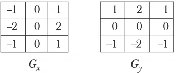
Sobel Operator was discovered by Irwin Sobel. It uses a 3×3 convolution mask which is the x and y direction on the image. It is discovered at first derivative level. The horizontal and vertical pixel masks for Sobel Operator are given as:

–1 0 1 1 2 1

–2 0 2 0 0 0

–1 0 1 –1 –2 –1

G_x G_y

The mask will be moved until all the images and each value, R, will be kept into an output array, which is located at the mask centre. The formula to find the gradient magnitude is:

|G| = |Gx| + |Gy| (1) where the calculation for Gx and Gy value:

Gx= (a₂+ ca₃+a₄) – (a₀+ca₇+ a₆)

(2)

Gy= (a₀+ ca₁+a₂) – (a₆+ c a₅+a₄) where the constant c=2.

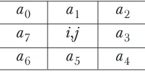
Figure 1 shows the neighbourhood pixel to describe the Sobel Operator concept.

Figure 1 Neighbourhood pixel describe Sobel Operator concept

a₀ a₁ a₂

a₇ i,j a₃

a₆ a₅ a₄

(b) Prewitt Operator

Prewitt Operator is pioneered by Judy Prewitt [8] and is based on the central difference concept.

∂ ≈ − −

∂ [ ( + 1, ) I( 1, )/2]

I

I x y x y

(6)

This will produce a convolution mask, –1 0 1

Prewitt Operator is much more sensitive to noise effect [8]. Thus, averaging process will be used to solve the noise problem. The convolution mask for Prewitt Operator have been implemented after averaging process at x and y axis for ∂/∂x and ∂/∂y.

The equation for Prewitt Operator and Sobel Operator is quite similar except for the value of constant c=1.

(c) Robert Cross Operator

Robert Cross Operator uses 2×2 convolution masks. It uses {+1,–1} operator that will calculate the value I xi( )−I xj( ) for (i,j) pixel at environs pixel. Mathematically, this equation is known as “forward differences” [8].

∂ ≈ + −

∂ ( 1, ) ( , ) I

I x y I x y

x (4)

Convolution mask of Robert Cross Operator is illustrated in Figure 2.

Calculation for gradient magnitude is given as:

= 2 + 2

( 1* ) ( 2 * )

G g f g f (5)

(2) Laplacian Operator

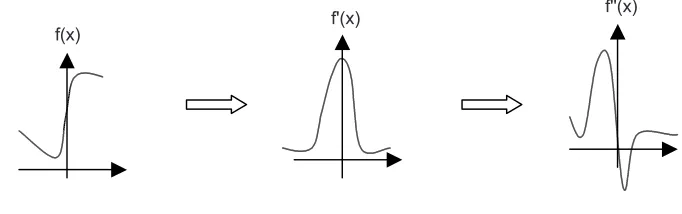
Laplacian Operator is a second order derivative, where the value of edge pixel at the first derivative is referred to as zero-crossing at second order derivative, as shown in Figure 3.

Figure 2 Convolution mask using Robert Cross Operator

+1

–1

g1

+1 –1

g2

Figure 3 Second order of Laplacian Operator

f(x)

f'(x) f''(x)

(7)

3.2.4 Niblack Binarization Technique

This technique is suitable to discard shadow [2]. It will obtain the T value by calculating the standard deviation and average for the chosen area, and add the average to, the multiply value between the weightage, which has a fixed value with the standard deviation.

T(x,y) =ω×σ (x,y) +µ (x,y) (6) where,

T- threshold at pixel (x,y) ; σ (x,y)- standard deviation

ω- weightage (fixed value) ; µ (x,y)- average for the pixels among pixel (x,y) The value of the weightage is –0.2 while the window that is been used is free and constantly changing. The processing time for a big window (15×15) is much faster than the small window but the result is much better by producing a great binary image.

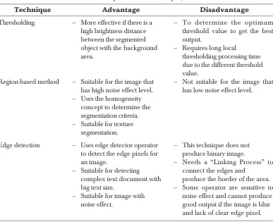
3.3 Comparison of the Techniques/Method

Table 1 Comparison of the techniques/method

Technique Advantage Disadvantage

Thresholding – More effective if there is a – To determine the optimum high brightness distance threshold value to get the best between the segmented output.

object with the background – Requires long local

area. thresholding processing time

due to the different threshold value.

Region-based method – Suitable for the image that – Not suitable for the image that has high noise effect level. has low noise effect level. – Uses the homogeneity

concept to determine the segmentation criteria. – Suitable for texture

segmentation.

Edge detection – Uses edge detector operator – This technique does not to detect the edge pixels for produce binary image.

an image. – Needs a “Linking Process” to

– Suitable for detecting connect the edges and

complex text document with produce the border of the area. big text size. – Some operator are sensitive to – Suitable for image with noise effect and cannot produce

(8)

4.0 HYBRID TECHNIQUE

River identification process from aerial photo involves 3 main processes which are:

(1) Obtaining grey scale image with 8 bit/pixel format. This means, each pixel has the possibility of 256 types of grey color from white to black. The size of the image is 500×700 pixel and the image file format that can be processed by the system are JPEG, GIF, and BMP format.

(2) Doing the thresholding technique to decrease the number of weak edge pixel and the non-maximum edge pixel. It is also to decrease the effect of noise [5]. All pixels on the image are tested. Some threshold value, θ, are identified and tested to obtain the best threshold value; θ= 100, 128, 150, and 180.

θ ≥ 

=  

1

1 if ( ,1) ( ,1)

0 otherwise e k

E k ₍₇₎

where,

e(k,1) – output from thresholding technique

(3) Detecting the location of the river’s edge pixel by using the edge detection method. Edge detection is used because the location of the river on the grey scale image is experiencing an intensity changes (0 to 255 or else). Edge pixel can be described according to:

(a) The pixel strength is referring to the magnitude of steaming. (b) The edge direction is referring to the degree of steaming.

The operator that is involved is Sobel Edge Detector because it is suitable for an image that has low noise effect. For a higher noise effect, a bigger mask is required. This operator consists of 2 convolution masks, which are G_x (vertical) and G_y

(horizontal), as shown in Figure 4.

–1 0 1 1 2 1

–2 0 2 0 0 0

–1 0 1 –1 –2 –1

G_x G_y

Figure 4 Sobel convolution mask

The formula to calculate the gradient magnitude is:

(9)

Gx= (a₂+ca₃+a₄) – (a₀+ca₇ +a₆)

Gy= (a₀ +ca₁+a₂) – (a₆+ ca₅+a₄) (9) where the constant c=2.

The formula for edge direction calculation is:

θ= arctan(Gy/Gx)

Figure 5 Shows the neighbourhood pixel to describe the Sobel Operator concept

a₀ a₁ a₂

a₇ [i,j] a₃

a₆ a₅ a₄

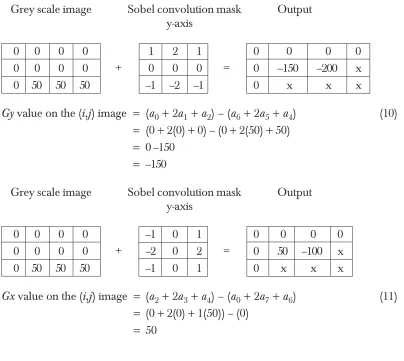
To summarize, Sobel Operator functions are described as follow:

Grey scale image Sobel convolution mask Output y-axis

0 0 0 0 1 2 1 0 0 0 0

0 0 0 0 + 0 0 0 = 0 –150 –200 x

0 50 50 50 –1 –2 –1 0 x x x

Gy value on the (i,j) image = (a₀+ 2a₁ +a₂) – (a₆+ 2a₅+a₄) (10) = (0 + 2(0) + 0) – (0 + 2(50) + 50)

= 0 –150 = –150

Grey scale image Sobel convolution mask Output y-axis

0 0 0 0 –1 0 1 0 0 0 0

0 0 0 0 + –2 0 2 = 0 50 –100 x

0 50 50 50 –1 0 1 0 x x x

Gx value on the (i,j) image = (a₂+ 2a₃ +a₄) – (a₀+ 2a₇+a₆) (11) = (0 + 2(0) + 1(50)) – (0)

(10)

This project can be successive with an assumption that the degree of photo acquired is 90° and the viewing degree are ignored. Besides that, there are a few limitations such as the aerial photo picture is in grey scale format 8 bit/pixel, must not be blurry and influenced by a noise. The output is also unsatisfactory if the image does not contain sharp edges.

5.0 IMPLEMENTATION AND RESULT 5.1 Reading Image File

The algorithm to read the image is:

For I = 0 to y For j = 0 to x

Pixel = GetPixel (j,i); Warna = Pixel&mod256; ImagePixels(i,j) = warna;

The GetPixel ( ) function is to get the intensity value for each pixel. This intensity value will be kept in an array using ImagePixel(i,j) function. The maximum value for the array content is 700 and 600 pixels for the x axis (i) and y axis (j) value.

5.2 Thresholding Technique: Discard the Weak Pixels at Aerial Photo Picture

For a simple implementation, thresholding technique will produce 2 outputs which represent the object and the background area. The object is represented by white color (255) while the background area is in black (0).

The algorithm for thresholding technique is:

For i = 1 to y–1 For j = 1 to x–1

threshold = ImagePixels(0,i,j);

If(threshold>threshold_value) then threshold_value=255; SetPixelV,j,i,RGB(255, 255, 255);

If(threshold<threshold_value) then threshold_value=0; SetPixelV,j,i,RGB(0, 0, 0);

(11)

5.3 Result of Thresholding Technique

The outcome result using the thresholding techniques can be referred in Appendix A. According to the thresholding results, it can be concluded that:

For threshold value; θ = 128 , decrease the non-edge pixel θ = 150 , a lot of loss occurred

θ = 110, noise effect happened that will decrease the percentage of success of hybrid technique.

Therefore, the best threshold value is θ= 128.

5.4 Edge Detection: Identifying the Edge Pixel Location of the River on the Image

5.4.1 Sobel Edge Detector

Sobel mask works vertically and horizontally on the image where it moves according to each orientation. Sobel Edge Detection can produce an output that is not highly influence by noise effect but takes time to process.

Algorithm for Sobel Edge Detection:

For i=1 to y For j=1 to x

kernel=abs((ImagePixels(i+1,j+1)+(2*ImagePixels(i+1,j))+ImagePixels(i+1,j–1))_

–ImagePixels(i–1,j+1)+ (2*ImagePixels(i–1,j))+ ImagePixels(i–1,j–1)))_

+Abs((ImagePixels(i–1,j+1)+(2*ImagePixels(i,j+1))+ImagePixels(i+1,j+1))_ –ImagePixels(i–1,j–1)+ (2*ImagePixels(i,j–1))+ ImagePixels(i+1,j–1)))

If kernel<0 then kernel=0; SetPixelV,j,i,RGB(0, 0, 0); If kernel>255 then kernel=255;

SetPixelV,j,i,RGB(255, 255, 255);

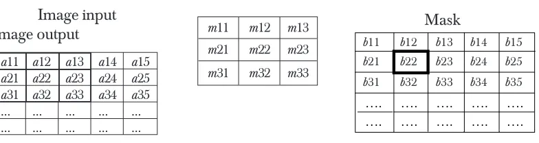
Sobel convolution mask will move across the area at image input, changes the pixel value and moves to the right pixel until it reaches the last row. After that, the convolution mask will start at the next row.

b22 =a11(m11)+a13(m13)+a21(m21)+a22(m22)+a23(m23) +

a31(m31)+a32(m32)+a33(m33) (12)

(12)

Mask

Figure 6 Sobel convolution mask

Image input Image output

a11 a12 a13 a14 a15

a21 a22 a23 a24 a25

a31 a32 a33 a34 a35

… … … … …

m11 m12 m13

m21 m22 m23

m31 m32 m33

Gx and Gy values are counted and modulated using abs() function. The Gx and Gy

values are added to get the gradient magnitude.

5.4.2 Prewitt Edge Detector

Prewitt Edge Detector consists of 2 convolution masks and it works and produces output which is similar to Sobel Operator.

The algorithm for Prewitt Edge Detector is:

kernel=Abs((ImagePixels(i+1,j+1)+(ImagePixels(i+1,j))+ImagePixels(i+1,j–1))_

–ImagePixels(i–1,j+1)+ (2*ImagePixels(i–1,j))+ ImagePixels(i–1,j–1)))_

+Abs((ImagePixels(i–1,j+1)+(ImagePixels(i,j+1))+ImagePixels(i+1,j+1))_ –ImagePixels(i–1,j–1)+ (ImagePixels(i,j–1))+ ImagePixels(i+1,j–1)))

5.4.3 Laplacian Edge Detector

This consists of a combination of 2 convolution masks. This operator is easily influenced by noise effect. Edge pixel is identified when there is zero-crossing at the second derivative.

The algorithm for Laplacian Edge Detector is:

kernel=(–4*ImagePixels(i,j)+(ImagePixels(i–1,j)) +ImagePixels(i+1,j))

+ImagePixels(I,j–1) +ImagePixels(I,j+1)

…. …. …. …. ….

b11 b12 b13 b14 b15

b21 b22 b23 b24 b25

(13)

5.4.4 Robert Cross Edge Detector

This operator consists of 2×2 convolution masks and it is the easiest and fastest edge detector. It is sensitive to noise effect because it only uses some pixels to count the gradient and produce weak edge pixel, except if there are high intensity changes. The algorithm for Robert Cross Edge Detector is:

Kernel=Abs(ImagePixels(i,j)–ImagePixels(i+1,j+1))+Abs(ImagePixels(I,j+1)– ImagePixels(i+1,j))

5.5 Result of Edge Detection

The result consists of Sobel, Prewitt, Laplacian, and Robert Cross while the resolutions are 75, 200, and 360, are reported in Appendix B.

According to the edge detection result, Sobel Operator can produce the best output because it is affected by the noise and can produce sharp edges while involving more complex calculation.

5.6 Hybrid Technique

The steps taken for the hybrid technique are:

(1) Do the thresholding process first to discard the weak edge pixels and unnecessary noise.

(2) Followed by edge detection process on the threshold image to detec the edge pixel for the river.

5.7 Result of Hybrid Technique

(14)

better result compared to other techniques because it can discard the edge pixels that are not represented by the river area, as reported in Appendix C.

6.0 CONCLUSION

In this study, the hybrid technique (thresholding and edge detection) had been implemented to identify the river from aerial photo and conducted some experiments to get the best threshold value. Results showed that the best threshold value is 128 and Sobel edge detection is the best operator. The selection of the suitable threshold value and edge detector will give the right desired output. Simultaneously, a variation of image resolution will also contribute to the success of the output.

Results from this study showed that, if the smoothing process is done before, it will decrease the noise effect and gives a better and clearer output. As it can decrease the noise effect, it also contributes to the loss of image’s data.

Conclusively, the technique that utilises threshold and edge detection shows object such as river can be identified clearly with higher clarity.

REFERENCES

[1] Rangsanseri, Y., and S. Rodtook. Comparative Study of Thresholding Technique of Grey Level Document Image Binarization. IEEE Catalogue No. 01CH37239.

[2] Sauvola, J., and M. Pietikainen. 1999. Adaptive Document Image Binarization. Pattern Recognition 33(2000). 255-236.

[3] Arnaldo, J. Abrantes, and J. S. Marques. 1996. A Class of Constrained Clustering Algorithms For Object Boundary Extraction. IEEE Trans. On Image Processing. 5(11).

[4] K. Haris, S. N. Efstratiadis, N. Maglaveras, and A. K. Katsaggelos. 1998. Hybrid Image Segmentation Using Watershed and Fast Region Merging. IEEE Trans. On Image Processing. 7(12).

(15)

APPENDIX A

RESULT OF THRESHOLDING TECHNIQUE

(1) Image 1

Resolution: 75dpi Threshold value: θ

(16)

(3) Image 3

Resolution: 360dpi Threshold value: θ (2) Image 2

θ = 150 θ= 180 θ = 110 θ= 128

(17)

APPENDIX B

RESULT OF EDGE DETECTION

(1) Image 1

Resolution: 75dpi Time: T

Sobel Edge Detection T = 2.844s

Laplacian Edge Detection T = 2.844s

Prewitt Edge Detection T = 3.023s

(18)

(2) Image 2

(3) Image 3

Robert Cross Edge Detection T = 2.463s

(19)

APPENDIX C

RESULT OF HYBRID TECHNIQUE

(1) Image 1

θ = 110

θ = 150

θ= 128

(20)

(2) Image 2

(3) Image 3

θ = 110

θ = 150

θ = 110

θ= 128

θ= 180

θ= 128