Volume 39– No.15, February 2012
A Comparative Analysis of Thresholding and Edge
Detection Segmentation Techniques
Jaskirat Kaur
Student UIETChandigarh
Sunil Agrawal
Assistant prof.,UIETPanjab university Chandigarh
Renu Vig
Director, UIET Panjab universityChandigarh
ABSTRACT
Thresholding and edge detection being one of the important aspects of image segmentation comes prior to feature extraction and image recognition system for analyzing images. It helps in extracting the basic shape of an image, overlooking the minute unnecessary details. In this paper using image segmentation (thresholding and edge detection) techniques different geo satellite images, medical images and architectural images are analyzed. To quantify the consistency of our results error measure is used.
General Terms
Image segmentation, edge detection, thresholding
Keywords
𝑒𝑟𝑚𝑠, Error measures, algorithms
1.
INTRODUCTION
Image segmentation techniques play an important role in image recognition system. It helps in refining our study of images. One part being edge and line detection techniques highlights the boundaries and the outlines of the image by suppressing the background information. They are used to study adjacent regions by separating them from the boundary.
The main problem of quantifying different edge detectors is that there is no unique way of studying an image. For example, each person has its own perception of segmenting and analyzing the image. If we reach at two different results arising from the same image then one single particular technique will be declared inconsistent [1].
This paper presents a quantitative study of different edge detection and thresholding techniques. Comparison is done on images from medical, geo spatial and architectural fields. Edge detectors like prewitt, canny and sobel were implemented and tested on various images from these fields. The characteristic used to measure the consistency of these edge detectors is 𝑒𝑟𝑚𝑠, which is root mean square error
between the input image and the output image. This measure allows a principled comparison between different results generated by the edge detectors.
This paper is organized a follows: section 2 related work is briefly presented. Section 3 describes the image segmentation and the edge detectors used. Section 4 presents the experimental results. Section 5 concludes the paper.
2.
RELATED WORK
There is a huge literature on segmentation dating back to decades, with applications in myriad areas. In this section,
image is segmented and simply sorted to object and background by setting a threshold. It is easy to get good results by threshold segmentation. However, if there is complex information in an image, the threshold algorithm is definitely not suitable. Edge detectors have been evaluated based on average risk [9]. It is the performance measure based on Bayesian decision theory. In this performance, edge detector is context dependent which makes it non-trivial. Edges are detected for the images in spatial domain and edge detectors are evaluated based on the relative frequencies of the edge detected pixels and edge differences.
3.
IMAGE SEGMENTATION
Image Segmentation is the process of dividing a digital image into constituent regions or objects [4]. The purpose of segmentation is to simplify the representation of an image into that which is easier to analyze. Image segmentation is typically used to locate objects and boundaries in images. Segmentation algorithms are based on the two basic properties of an image intensity values: discontinuity and similarity. To study discontinuities in an image we divide image based on the abrupt changes in intensity, such as edges.
3.1
Edge Detectors
Edge detection is the most common approach for detecting meaningful discontinuities in intensity values. The edge is a boundary between two regions with relatively distinct gray level properties. Such discontinuities are detected by using first and second order derivatives. The first-order derivative in image processing is the gradient defined as below. The gradient of an image f(x,y) at location (x,y) is the vector[3]:
∇𝑓 =
𝐺𝑥𝐺𝑦
=
𝜕𝑓 /𝜕𝑥
𝜕𝑓 /𝜕𝑦
The gradient vector points in the direction of maximum rate of change of f at (x,y). In edge detection, an important parameter is the magnitude of this vector.
|
∇𝑓|
=
𝐺
𝑥2+ 𝐺
𝑦2The gradient takes it’s maximum rate of increase of f(x,y) per unit distance in the direction of f . To simplify computation, ignoring square root approximates this quantity.
|
∇𝑓|
=|
𝐺
𝑥| + |𝐺
𝑦|
Volume 39– No.15, February 2012
𝛼 𝑥, 𝑦 = 𝑡𝑎𝑛
−1𝐺
𝑦𝐺
𝑥The frequently used edge detection techniques in image segmentation are:
(1) Sobel Edge Detection, (2) Prewitt Edge Detection and (3) Canny Edge Detection. (4) Roberts Edge Detection
The description of these methods is as follows.
(1) Sobel Edge Detection
Sobel edge detector uses the masks as shown in the figure below to digitally approximate the first order derivatives Gx and Gy [3].
G=
𝐺
𝑥2+ 𝐺
𝑦2 1/2={
𝑧
7+ 2𝑧
6+ 𝑧
9− 𝑧
1+ 2𝑧
4+ 𝑧
72
+
𝑧
3+ 2𝑧
6+ 𝑧
9− 𝑧
1+ 2𝑧
4+ 𝑧
72
}
1/2In its most common usage, the input to the operator is a gray scale image, as is the output. Pixel values at each point in the output represent the estimated absolute magnitude of the spatial gradient of the input image at that point.
𝑧
1𝑧
2𝑧
3𝑧
4𝑧
5𝑧
6𝑧
7𝑧
8𝑧
9Image neighbourhood
G
x=(
𝑧
7+ 𝑧
8+ 𝑧
9)-
(
𝑧
1+ 𝑧
2+ 𝑧
3)
Sobel mask
G
y=(
𝑧
3+ 2𝑧
6+ 𝑧
9)
-
(
𝑧
1+ 2𝑧
4+ 𝑧
7)
(2) Prewitt Edge Detector
The prewitt edge detector uses the masks shown in figure below to digitally approximate the first derivatives Gx and Gy. The parameters of prewitt edge detector are similar to Sobel parameters. Though Prewitt edge detector is simpler to implement than the Sobel detector, but it tends to produce somewhat noisier results. The Prewitt operator measures two components namely the vertical edge component, which is calculated using kernel Gx and the horizontal edge component, which is calculated using kernel Gy. |Gx| + |Gy| gives an indication of the intensity of the gradient in the current pixel.
G
x=(
𝑧
7+ 𝑧
8+ 𝑧
9)
-
(
𝑧
1+ 𝑧
2+ 𝑧
3)
Prewitt mask
G
x=(
𝑧
7+ 𝑧
8+ 𝑧
9)
-
(
𝑧
1+ 𝑧
2+ 𝑧
3)
(3) Canny Edge Detector
The canny edge detector is the most powerful edge detector. This technique finds edges by separating noise from the image before finding the edges of the image. It does not affect the features of the edges of the image. The method of finding edges using canny edge detector is as follows [7]:
(a) The image is smoothened using the Gaussian filter, to reduce noise.
(b) The local gradient,
G(x,y)=
𝐺
𝑥2+ 𝐺
𝑦2 1/2and edgedirection
𝛼
(x,y)=tan
-1(G
y/Gx),
are computed at eachpoint. The advantage of using this method is that any of the Prewitt, Sobel, Roberts technique can be used to compute Gx and Gy. Then edge point is a point whose strength is locally maximum in the direction of the gradient.
(c) The edge points detected in step 2 give rise to ridges in the gradient magnitude image. The algorithm then tracks along the top of these ridges and sets to zero all pixels that are not actually on the ridge top so as to give a thin line in the output, a process which is known as nonmaximal suppression. The ridge pixels are then thresholded using two thresholds, T1 and T2, with T1<T2. Ridge pixels with values greater than T2 are said to be strong edge pixels. Ridge pixels with values between T1 and T2 are said to be weak edge pixels.
(d) In the last step the algorithm performs edge linking by incorporating the weak pixels that are 8-connected to the strong pixels.
(4) Roberts Edge Detection
The Roberts edge detector computes 2-D spatial gradient on the image. It highlights regions of high spatial frequency, which corresponds to edges. Input to the operator is a gray scale image, as is the output. Pixel values at each point in the output represents the estimated absolute magnitude of the spatial gradient of the input image at that point [4]. The mask used by the Roberts edge detector used is shown in the figure below.
-1
-2
-1
0
0
0
1
2
1
-1
0
1
-2 0
2
-1 0
1
-1
-1
-1
0
0
0
1
1
1
-1
0
1
-1
0
1
Volume 39– No.15, February 2012
-1
0
0
1
G
x=
𝑧
9− 𝑧
50
-1
1
0
G
y=
𝑧
8− 𝑧
63.2 Thresholding
Thresholding is one of the simplest image segmentation techniques. A threshold is chosen according to the application for which it is applied. If one particular image has light objects in the dark background, one way to extract the objects in the background is to select a threshold T that separates background and foreground objects [5]. The point for which f(x,y) ≥T is called an object point; otherwise the point is called as background point.
g(x, y) = 1 𝑖𝑓 𝑓 𝑥, 𝑦 ≥ 𝑇
0 𝑖𝑓 𝑓 𝑥, 𝑦 < 𝑇
There are numerous ways of selecting threshold like visual inspection, trial and error but these methods consume a lot of time .The best way for choosing threshold automatically is given in the following procedure [10]:
(a) Select an initial estimate for T. Generally it is the mid point between the minimum and maximum intensity values of the image.
(b) Segment the image using T. This will produce two groups of pixels: G1, consisting of all pixels with intensity values ≥ T, and G2, consisting of pixels with values < T.
(c) Then compute the average intensity values µ1 and µ2 for
the pixels in regions G1 and G2.
(d) In the last step compute a new threshold value:
T = 1/2 (µ1 + µ2)
(e) Repeat the steps from b to d until the difference in T in successive iterations is smaller than a predefined parameter.
3.3 Root Mean Square Error
The Root mean square error (𝑒𝑟𝑚𝑠) is a measure, which calculates the average magnitude of the error. The equation for the 𝑒𝑟𝑚𝑠 is given below. The difference between the
forecast and corresponding observed values are each squared and then averaged over the sample. Finally, the square root of the average is taken. Since the errors are squared before they are averaged, the 𝑒𝑟𝑚𝑠 gives a relatively high weight to large
errors. The input image is represented as f (x,y), output image
𝑓 (x,y) and the error with e(x,y).
𝑒 𝑥, 𝑦 = 𝑓 (𝑥, 𝑦) − 𝑓(𝑥, 𝑦)
And the total error between two images is
𝑀−1
𝑥=0 [𝑓 𝑁−1
𝑦=0
𝑥, 𝑦 − 𝑓(𝑥, 𝑦)]
𝑒
𝑒𝑟𝑚𝑠 = 1/𝑀𝑁[
𝑀−1
𝑥=0 [ 𝑓 𝑁−1
𝑦=0
(𝑥, 𝑦) − 𝑓(𝑥, 𝑦)] 2] 1/2
4. EXPERIMENTAL RESULTS
In this section, the results are presented which are obtained by applying different edge detectors: prewitt, canny, sobel and thresholding segmentation techniques. The error measure calculated and compared in this section.
The experiments were made on number of images [11] and one from each field is shown over here and the results are compared.
Medical images:
Original Image (Brain tumour)
Segmentation using prewitt
𝑒𝑟𝑚𝑠=292.5418
Segmentation using canny
𝑒𝑟𝑚𝑠=292.0325 (Best Result)
Segmentation using sobel
𝑒𝑟𝑚𝑠=292.6503
Segmentation using thresholding
𝑒𝑟𝑚𝑠=303.9847
For brain tumours canny edge detector works best to detect tumours.
Figure 1.
Original Image (lungs)
Original image (Brain tumour)
Segmentation using prewitt Segmentation using canny
Segmentation using sobel image using thresholding
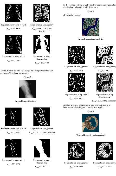
Volume 39– No.15, February 2012
Segementation using prewitt
𝑒𝑟𝑚𝑠=245.5808
Segmentation using canny
𝑒𝑟𝑚𝑠=245.2815 (Best Result)
Segmentation using sobel
𝑒𝑟𝑚𝑠=245.5892
Segmentation using thresholding
𝑒𝑟𝑚𝑠= 262.7583
[image:4.595.52.534.57.789.2]For fracture in the ribs canny edge detector provides the best amount of detail and least error.
Figure 2.
Original Image (fracture)
Segementation using prewitt
𝑒𝑟𝑚𝑠=273.7957
Segmentation using canny
𝑒𝑟𝑚𝑠=273.7253(Best Results)
Segmentation using sobel
𝑒𝑟𝑚𝑠=273.8051
Segmentation using thresholding
𝑒𝑟𝑚𝑠=289.4375
In the leg bone where actually the fracture is canny provides the detailed information with least error.
Figure 3.
Geo-spatial images:
Original Image (geo-satellite)
Segmentation using prewitt
𝑒𝑟𝑚𝑠=279.8371
Segmentation using canny
𝑒𝑟𝑚𝑠=279.6371
Segmentation using sobel
𝑒𝑟𝑚𝑠=279.8456
Segmentation using thresholding
𝑒𝑟𝑚𝑠= 279.6345(Best results)
Another example of separating land and river going in between thresholding provides the best results
Figure 4.
Original Image (remote sensing)
Segmentation using prewitt
𝑒𝑟𝑚𝑠=276.2681
Segmentation using canny
𝑒𝑟𝑚𝑠=276.2885
Segmentation using prewitt Segmentation using canny
Segmentation using sobel image using thresholding
Original image (fractured bone)
Segmentation using prewitt Segmentation using canny
Segmentation using sobel image using thresholding
Original image (geo satellite)
Segmentation using prewitt Segmentation using canny
Segmentation using sobel image using thresholding
Original image (remote sensing)
Volume 39– No.15, February 2012
Segmentation using sobel
𝑒𝑟𝑚𝑠=276.2977
Segmentation using thresholding
𝑒𝑟𝑚𝑠=276.1223(Best results)
Clearly we can study the shape and separate water from the hotel area by thresholding.
Figure 5.
Architectural images:
Original Image (architecture image)
Segmentation using prewitt
𝑒𝑟𝑚𝑠=202.3350(Best results)
Segmentation using canny
𝑒𝑟𝑚𝑠=202.3453
Segmentation using sobel
𝑒𝑟𝑚𝑠=202.3440
Segmentation using thresholding
𝑒𝑟𝑚𝑠=202.3434
[image:5.595.68.273.69.187.2]To study the architecture of the building we need outlines, which are best provided by the prewitt edge detector.
Figure 6.
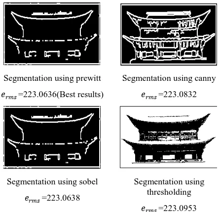
Segmentation using prewitt
𝑒𝑟𝑚𝑠=223.0636(Best results)
Segmentation using canny
𝑒𝑟𝑚𝑠=223.0832
Segmentation using sobel
𝑒𝑟𝑚𝑠=223.0638
Segmentation using thresholding
𝑒𝑟𝑚𝑠=223.0953
For the basic outline of the architecture we can either use prewitt or sobel with the minute difference in 𝑒𝑟𝑚𝑠.
Figure 7.
Original Image (house architecture image)
Segmentation using prewitt
𝑒𝑟𝑚𝑠=212.1172
Segmentation using canny
𝑒𝑟𝑚𝑠=212.9409
Segmentation using sobel
𝑒𝑟𝑚𝑠=212.1175(Best results)
Segmentation using thresholding
𝑒𝑟𝑚𝑠=212.9234
Here also prewitt or sobel provides the almost equal results.
Figure 8.
The images taken over here were implemented over many other similar images to detect particular areas. Some of them as an example to the field are added in this section. Based on
Segmentation using sobel image using thresholding
Original image (architecture image)
Segmentation using prewitt Segmentation using canny
Segmentation using sobel image using thresholding
Original image (Traditional architecture image)
Segmentation using prewitt Segmentation using canny
Segmentation using sobel image using thresholding
Original image (architecture image)
Segmentation using prewitt Segmentation using canny
Segmentation using sobel
[image:5.595.316.538.70.285.2] [image:5.595.315.537.434.670.2] [image:5.595.116.218.669.736.2]Volume 39– No.15, February 2012
we need to use other detector which provides the best results with the least 𝑒𝑟𝑚𝑠 as shown in above tables.
5. CONCLUSION
This paper resulted a comparison of thresholding, different edge detection techniques on images from different fields. Observation was made that each type of image has different area to be analyzed. In this paper, images were examined using different techniques and the ones providing accurate results were identified. In the future work, the comparative study will be made by taking different clustering techniques used in image segmentation.
6. REFERENCES
[1] Alina Doringa, Gabriel Mihai, Dan Burdescu, “comparison of two image segmentation algorithms” Second international conference on advances in multimedia, IEEE computer society, pp. 185-190 (2010)
[2] Mr Salem Saleh Al-amri, Dr. N.V. Kalyankar, Dr.Khamitkar S.D “Image segmentation by using edge detection”, International journal on computer science and engineering, vol. 02, No. 03, 2010, pp. 804-807
[3] N.Senthilkumaram, R.Rajesh “Edge detection techniques for image segmentation-A survey of soft computing approach”, International journal of recent trends in engineering , vol.1, No.2, May 2009,pp. 250-254
[4] Steven L Eddins, Richard E.woods, Rafael C “digital image processing” (2009)
[5] Huang, Yourui; Wang, Shuang “Multilevel thresholding Methods for image segmentation with otsu based on QPSO”, Image and signal processing, CISP 2008, vol. 3,pp.701-705
[6] Shiping Zhu, Xi Xia, Qingrong Zhang, kamel Belloulata “An image segmentation in image processing based on threshold segmentation”, Third international IEEE conference on signal-Image Technologies and internet- based system, SITIS 2007 ,pp. 673-678
[7] Kalelia, F.; Aydina, N.; Ertas, G.;Gulcur, H.O.; “An adaptive approach to the segmentation of DCE-MR images of the breast: comparison with classical thresholding algorithms” ,Computational intelligence on image and signal processing. CIISP 2007,IEEE symposium, pp. 375-379
[8] Raman Maini, Dr.Himanshu Aggarwal “Study and comparison of various edge detection techniques”, International journal of image processing, vol. 3: issue(1)
[9] Hong Shan Neoh, Asher Hazan chuk “Adaptive edge detection for real-time video processing using FPGAs”, 101 innovation drive, San jose, CA
[10]Spreeuwers, L.J.; Van der Heijden , F.; “Evaluation of edge detection using average risk”, Pattern recognition , vol. 3 ,Conference on Image ,speech and signal analysis, pp. 771-774, (2002)