Volume 2009, Article ID 623537,12pages doi:10.1155/2009/623537
Research Article
Discrete-Time Second-Order Distributed
Consensus Time Synchronization Algorithm for
Wireless Sensor Networks
Gang Xiong and Shalinee Kishore
Department of Electrical and Computer Engineering, Lehigh University, Bethlehem, PA 18015, USA
Correspondence should be addressed to Shalinee Kishore,[email protected]
Received 14 April 2008; Accepted 7 September 2008
Recommended by Erchin Serpedin
This paper proposes a novel discrete-time second-order distributed consensus time synchronization(SO-DCTS) algorithm for wireless sensor networks. The consensus properties and convergence rates of the SO-DCTS algorithm are analyzed for both directed and undirected networks. Additionally, the convergence region and optimal convergence rate of the SO-DCTS algorithm are determined for undirected networks and this convergence rate is shown to be superior to that of thefirst-orderDCTS (FO-DCTS) algorithm under careful algorithm design. Furthermore, the asymptotic expectation and mean square synchronization error are investigated for the SO-DCTS algorithm when there is Gaussian delay between network nodes. Finally, simulation results are provided to verify these analytical results.
Copyright © 2009 G. Xiong and S. Kishore. This is an open access article distributed under the Creative Commons Attribution License, which permits unrestricted use, distribution, and reproduction in any medium, provided the original work is properly cited.
1. Introduction
Wireless sensor networks are typically comprised of inex-pensive, small-sized, power-limited terminals. In a variety of applications, these sensor nodes are collectively required to maintain accurate time synchronization, for example, moving object acquisition and tracking, habitat monitoring, reconnaissance and surveillance, environmental monitoring, traffic control, and so forth [1]. This necessitates network algorithms that achieve and maintain global time synchro-nizationat all network nodes, that is, algorithms that align all network nodes to a common notion of time.
Due to imperfections in low-cost hardware nodes and the decentralized nature of wireless sensor networks, global time synchronization has been recognized as a particularly challenging task. Conventional synchronization protocols such as time-synchronization protocol for sensor networks (TPSNs) [2], reference broadcast synchronization (RBS) [3], and flooding time synchronization protocol (FTSP) [4] aim to performcentralizedglobal synchronization for all nodes in wireless sensor network [5]. These protocols achieve synchronization via time-stamped packet exchanges with a
root node or a data fusion center and are thus vulnerable to failure of these central nodes.
Recently, several distributed time synchronization algo-rithms have been proposed. One important class of such algorithms is referred to as distributed consensus time synchronization (DCTS) [6]. In the DCTS approach, a global time consensus can be sufficiently reached within a connected network by averaging pair-wise local time information at network nodes. In [7], Olfati-Saber et al, established a theoretical framework for the analysis of con-sensus synchronization algorithms. Later, a fully distributed, asynchronous DCTS algorithm was proposed in [8]; this scheme was designed to reach agreement on time offset and skew offset between network nodes using media access control (MAC) layer time-stamped packet exchanges. As an alternative, a physical layer-based DCTS algorithm was introduced in [9] by modeling sensor nodes as coupled discrete-time oscillators. In particular, the algorithm adopts instantaneous received powers as weighted coefficients when updating local clocks.
node is done using only current timing information, that is, via afirst-order DCTS (FO-DCTS) approach. In contrast, a
second-orderDCTS (SO-DCTS) algorithm would utilize not only current timing information but also that available from the previous iteration of the algorithm to update local clocks. Such an extension to the basic consensus algorithm was first reported for a continuous time approach in [10]. Subsequent papers have analyzed this second-order continuous time consensus method assuming fixed network topologies [11], time delay [12], and switching topologies [13]. In this paper, we apply the principles of the second-order consensus approach to the distributed timing synchronization problem in wireless sensor networks. Specifically, we propose a novel discrete-timeSO-DCTS algorithm for wireless sensor networks and examine its convergence properties.
The major contribution of this paper is the theoreti-cal analysis of the convergence characteristics of the SO-DCTS algorithm for both directed and undirected networks. Moreover, we investigate the convergence region and optimal convergence rate of the SO-DCTS algorithm in undirected networks and claim that the optimal convergence rate of the SO-DCTS algorithm is superior to that of the FO-DCTS algorithm under an appropriate algorithm design. Finally, we present the asymptotic expectation and mean square synchronization error of the SO-DCTS algorithm when the timing offset between network nodes is Gaussian distributed. This paper is outlined as follows.Section 2describes the system model and background for the proposed SO-DCTS algorithm. Section 3 presents the convergence properties of the SO-DCTS algorithm in directed and undirected networks. Section 4 discusses the convergence region and optimal convergence rate of the SO-DCTS algorithm in undirected networks. InSection 5, we present some conver-gence results for the SO-DCTS method when network nodes have Gaussian delay between each other. Simulation results are presented inSection 6, and we conclude our discussion inSection 7.
2. Background and System Model
2.1. Proposed SO-DCTS Algorithm. Timing information between network nodes can be exchanged either using time-stamped packets at the MAC layer or by estimating arrival times of neighboring nodes’ physical layer pulse signals. In the following, we describe the SO-DCTS method regardless of whether it is implemented at the MAC or physical layers. In each iteration of the SO-DCTS algorithm, each node processes and decodes the time-stamped message from its neighbors or estimates the arrival time of its neighbors’ pulse signals. Each node then updates its local clock using the weighted average of the current time differences between itself and its neighboring nodes as well as stored time differences from the previous iteration of the algorithm. It should be noted that in the SO-DCTS algorithm, each node needs to store time information from its neighbor nodes for both the previous and current iterations; this is in contrast to the FO-DCTS approach where only the current time information is processed in the current iteration.
The timing update rule of the SO-DCTS algorithm at each nodeiis given as
ti(k)=ti(k−1) +ε
j∈Ni
tj(k−1)−ti(k−1)
−γε
j∈Ni
tj(k−2)−ti(k−2)
,
(1)
whereti(k) is the local time at nodeiduring iterationk;Niis
the set of neighboring nodes that can communicate reliably with nodei;εis a constant step size;γis a constant for each iteration. We assume that initial conditions of the SO-DCTS algorithm areti(−1) = ti(0) = zi, where zi is initial time
offset for nodei. It is worth mentioning that whenγ=0, the SO-DCTS algorithm reduces to the FO-DCTS algorithm.
2.2. Network Model and Some Preliminaries. In the following, we model a wireless sensor network as a graphG=(V,E), consisting of a set of nnodes V = {1, 2,. . .,n} and a set of edgesE. Each edge is denoted ase = (i,j) ∈ E where
i∈Vandj∈Vare head and tail of the edgee, respectively. In a wireless sensor network, the presence of an edge (i,j) indicates that nodeican communicate with node jreliably. We assume here a connected graph; that is, there exists a directed path connecting any pair of distinct nodes in the network. Throughout our discussion, we assume a time-invariant and connected network unless otherwise stated.
Given this network model, we denote A = [ai j] as the
adjacency matrix ofGsuch that
ai j=
1, (i,j)∈E,
0, otherwise. (2)
Then, the in-degree and out-degree of a nodei(denoted as
cianddi, resp.,) are given asci=
n
j=1aji, anddi=
n j=1ai j.
Specifically, di is also equal to the number of neighbors of
nodeifrom which it can receive information reliably, that is,
di= |Ni|.
Next, we letLbe the graph Laplacian matrix ofGwhich is defined asL =D−A, whereD = diag(d1,d2,. . .,dn) is
the degree matrix of G. Given this matrixL, we can show thatL1=0, where1 =[1, 1,. . ., 1]T, and0=[0, 0,. . ., 0]T. In particular, for a connected graph, the rank ofLisn−1. Furthermore, for a balanced directed network, the in-degree and out-degree of a node are equal, that is,ci =di, thus we
see that1TL=0T.
For an undirected network, the presence of an edge (i,j) indicates that nodes i and j can communicate with each other reliably. Under this condition, we can also show that 1TL=0T. Additionally, in this case, L is a symmetric
positive semidefinite matrix (implying that its eigenvalues are nonnegative), and its eigenvalues can be arranged in increasing order as 0=λ1(L)< λ2(L)≤ · · · ≤λn(L) [14].
Let us define t(k) = [t1(k),t2(k),. . .,tn(k)]T. The
evolution of the SO-DCTS algorithm in (1) can be written as
t(k)=In−εL
with the initial conditionst(−1) = t(0) = z, wherez =
[z1,z2,. . .,zn]T. Here,Indenotes then×nidentity matrix.
3. Convergence Properties of
the SO-DCTS Algorithm
In this section, we investigate the consensus properties of the SO-DCTS algorithm in directed and undirected networks. Additionally, we discuss the convergence rate of the SO-DCTS algorithm in such networks.
3.1. Consensus Analysis of the SO-DCTS Algorithm. The main result regarding the average consensus property of the SO-DCTS algorithm in directed networks is stated in the following theorem.
Theorem 1. For a time-invariant, connected, directed net-work, consider the SO-DCTS algorithm,
t(k)=(In−εL)t(k−1) +γεLt(k−2), (4) consensus is achieved asymptotically, or equivalently,
lim whereρ(·)denotes the spectral radius of a matrix.
Proof. The proof of this theorem is similar to [11, 15].
Thus, the eigenvalues ofHare
λk(H)=
For a time-invariant, connected, directed network,Lhas only one eigenvalueλ1(L) = 0. Then, we know thatH has
two eigenvaluesλ1(H) = 1 and λ2(H) = 0. Additionally,
the eigenvalues ofH −J agree with those ofH except that
λ1(H)=1 is replaced byλ1(H−J)=0 [16]. Sinceρ(H−J)<
1, we see that the eigenvalues ofHstay inside the unit circle except forλ1(H)=1. Thus, we have
where Λ is the Jordan form matrix corresponding to eigenvalues λi(H)=/1 [16], wl and wr are left and right
eigenvectors ofH corresponding toλ1(H)=1, respectively,
andwT
rwl = 1. In particular, wl = (1/βT1)[βT 0T]T and
wr=[1T 1T]T. Pluggingwlandwrinto (10) and considering
the SO-DCTS algorithm in (7), we have
lim
This completes the proof.
According toTheorem 1, we see that in general, although average consensus is not achieved for directed networks, all nodes in the network can still reach a global agreement. By “average consensus” we mean that all nodes converge to the same timing which is determined by the average of the initial timing differences between the nodes. However, when the SO-DCTS algorithm is employed in either an undirected network or abalanceddirected network, average consensus can be achieved asymptotically. We show this via the following theorem.
Theorem 2. Consider the SO-DCTS algorithm in (4) in a time-invariant, connected, directed balanced network or a time-invariant, connected, undirected network, with initial conditionst(−1)=t(0)=z. Whenρ(H−J)<1, an average consensus is achieved asymptotically, or equivalently,
lim
k→ ∞ti(k)=
1
n1
Tz, ∀i∈V. (13)
We know that in a time-invariant, connected, directed balanced or undirected network,β= 1andK =(1/n)11T. The rest of proof is similar to that ofTheorem 1and thus omitted here.
convergence speed of the SO-DCTS algorithm is determined by the spectral radius ofH−J, which is similar to the FO-DCTS algorithm [17].
Let us define the global consensus value in each iteration asm(k) = (1/βT1)βTt(k). In the SO-DCTS algorithm, this
value remains invariant during each iteration since
m(k)=1/βT1βTIn−εL
t(k−1) +γεLt(k−2)
=m(k−1)= · · · =m(0).
(14)
We now define the disagreement vector asδ(k)=t(k)− m(k)1, which indicates the difference between the updated times and the global consensus times of the network nodes. Then, the evolution of the disagreement vector is obtained as
δ(k)=In−εL
δ(k−1) +γεLδ(k−2). (15) Given this dynamic of the disagreement vector, we note the following Lemma.
Lemma 1. For the SO-DCTS algorithm in (4) in a time-invariant, connected network with initial conditionst(−1) =
t(0) =zandα =ρ(H−J)<1, a global consensus is expo-nentially reached in the following form:
δ(k)2+δ(k−1)2
δ(0)2 ≤2α
2k, (16)
where·denotes the2norm of a vector.
Proof. Let us define the error vector ase(k)=[δT(k)δT(k−
1)]Twhich can be obtained frome(k)=ψ(k)−J
1ψ(k), where
J1=
K 0n×n
0n×n K
. (17)
Based on this definition, we see that the error vector results in the following evolution:
e(k)=(H−J1H)ψ(k−1)
=(H−J)ψ(k−1)−J1ψ(k−1)
=(H−J)e(k−1).
(18)
The above equation is valid because (H−J)J1=02n×2nand
J1H=J. Then, we have
e(k)2= (H−J)e(k−1)2≤α2e(k−1)2
≤ · · · ≤α2ke(0)2, (19)
which is equivalent to (16). This completes the proof. Therefore, we see that the convergence rate for the SO-DCTS algorithm in both directed and undirected networks is determined by the spectral radius ofH−J.
0 0.1 1 1.5 2 2.5 3 3.5 4
|
λk
(
H
)
|
1 0
−1
−2
−3
−4
−5 γ
0 0.5
1 1.5
2 2.5 3 ελn(L)
Convergence region
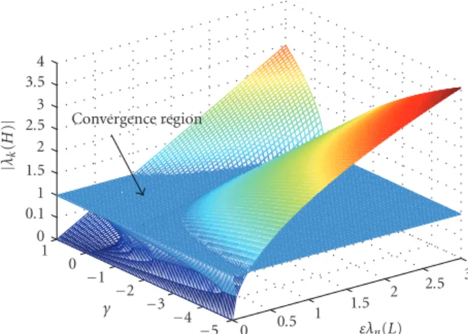
Figure 1: Convergence region for the SO-DCTS algorithm in undirected networks: three-dimensional view.
4. Convergence Region and Optimal
Convergence Rate for SO-DCTS Algorithm
in Undirected Networks
In this section, we investigate more specific convergence results (i.e., the convergence region and optimal convergence rate) for the SO-DCTS algorithm in undirected networks. Without loss of generality, we assume thatεandγare real values, andε >0.
4.1. Convergence Region for SO-DCTS Algorithm in Undi-rected Networks. From Theorem 2, we know that when
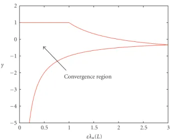
ρ(H −J) < 1, the SO-DCTS algorithm in an undirected network can achieve average consensus asymptotically. Let us define the convergence regionRto satisfyρ(H−J)<1. After some algebraic derivations (outlined inAppendix A), the convergence region for the SO-DCTS algorithm in undirected networks is
R=R†∪R‡, (20)
whereR† = {−1/(ελn(L))< γ < 1, 0 < ε < 1/λn(L)}, and
R‡ = {−1/(ελ
n(L)) < γ < 2/(ελn(L))−1, 1/λn(L) ≤ ε <
3/λn(L)}.
The convergence region of the SO-DCTS algorithm in undirected networks is shown in Figures 1 and 2 using a three-dimensional and two-dimensional perspective, respec-tively. We see that compared to the FO-DCTS algorithm where the range of the step sizeεis (0, 2/λn(L)), the range
ofεin the SO-DCTS approach increases to (0, 3/λn(L)).
4.2. Optimal Convergence Rate for SO-DCTS Algorithm in Undirected Networks. Next, we investigate the fastest convergence rate of the SO-DCTS algorithm based onεand
γ. Recall that in the FO-DCTS algorithm, the constant step sizeεopt,FOwhich minimizes convergence time is given as [15]
εopt,FO= 2
λn(L) +λ2(L).
Additionally, the convergence rate forεopt,FOis determined by
the second largest absolute eigenvalue of the Perron matrix [18], that is,
αopt,FO=λn(L)−λ2(L)
λn(L) +λ2(L).
(22)
As we show next, the convergence rate of the SO-DCTS algorithm can be superior to that of the FO-DCTS algorithm by choosing suitable ε and γ. However, as stated in the following lemma, the convergence rate of the FO-DCTS algorithm is faster under some circumstances.
Lemma 2. For the SO-DCTS algorithm in (4) in a time-invariant, connected, undirected network with initial condi-tionst(−1)=t(0) =zand(ε,γ)∈Rin(20), ifγ >0, the convergence rate of the SO-DCTS algorithm is less than that of the FO-DCTS algorithm with the optimal constant step size in
(21).
The proof of this lemma is omitted here since it can be readily extended from the following result. Consider two real values a and b with b > 0, then max{(1/2)|a+
√
a2+b|, (1/2)|a−√a2+b|}> a. Thus, we have|λk(H)|>
1−ελi(L), which implies|λk(H)|> αopt,FO.
Based on the above lemma, we see that there may exist possible choices ofεandγ(e.g., whenγ <0) such that the convergence rate of the SO-DCTS method is faster than the FO-DCTS algorithm. To see this, we formulate the following spectral radius minimization problem to find the optimalε
andγfor the SO-DCTS algorithm: minimize ρ(H−J)
subject to (ε,γ)∈R, γ <0. (23)
Using the steps outlined inAppendix B, the optimalεand
γto minimize (23) can be obtained as
εopt,SO= 3λn(L) +λ2(L)
λn(L)
λn(L) + 3λ2(L) ,
γopt,SO= −
λn(L)−λ2(L) 2
λn(L) + 3λ2(L)
3λn(L) +λ2(L) .
(24)
It is worth noting that (εopt,SO,γopt,SO) ∈ R‡. Recall
that the convergence rate for the SO-DCTS algorithm in undirected networks is determined by the spectral radius of
H−J, that is,
αopt,SO= λn
(L)−λ2(L)
λn(L) + 3λ2(L).
(25)
We see thatαopt,SO≤αopt,FOandαopt,SO=αopt,FOonly when
λ2(L)=λn(L). Thus, we have the following theorem for the
convergence rate of the SO-DCTS algorithm.
Theorem 3. For the SO-DCTS algorithm in (4)in a time-invariant, connected, undirected network with initial condi-tionst(−1) =t(0) =zand(ε,γ) ∈R in(20), there exists a pair of εand γ such that the convergence rate of the SO-DCTS algorithm is greater than or equal to that of the FO-DCTS algorithm with the optimal constant step size in(21).
−5
−4
−3
−2
−1 0 1 2
γ
0 0.5 1 1.5 2 2.5 3
ελn(L) Convergence region
Figure 2: Convergence region for the SO-DCTS algorithm in undirected networks: two-dimensional view.
5. SO-DCTS Algorithm with Gaussian
Delay in Undirected Networks
In this section, we investigate the convergence properties of the SO-DCTS algorithm in undirected networks when there is both deterministic and random (Gaussian) delay between network nodes during local time information exchange. In [19], we motivate why the Gaussian assumption is appropriate to model the undeterministic timing differences between nodes exchanging either MAC layer or physical layer timing information. We do not reiterate those arguments here but rather present convergence results for the SO-DCTS algorithm when such timing differences exist. We have separately examined the performance of the SO-DCTS algorithm considering alternate delay distributions, for example, exponential delay distribution [20]. Results show similar performance bounds as those presented in this paper for the Gaussian assumption. For this reason, we constrain our discussion here to the more common Gaussian delay model.
With Gaussian delay, the timing update rule of the SO-DCTS algorithm at each nodeiis given as
ti(k)=ti(k−1) +ε
j∈Ni
tj(k−1)−ti(k−1)
−γε
j∈Ni
tj(k−2)−ti(k−2)
,
(26)
wheretj(k)=tj(k) +Tdelay=tj(k) +Tc+Li j/c+vj(k);Tcis
a constant (deterministic) delay;Li j is the distance between
nodeiand j;cis light speed (thus,Li j/cis the propagation
delay between nodesiandj);vj(k) are independent identical
distributed (i.i.d) Gaussian random variables, with zero mean and variance σ2. Local time information exchange
between nodei and j under this delay model is shown in
Nodei ti(k) ti(k+ 1)
Nodej tj(k) ti(k+ 1)
Tc+Li j/c+vj(k) Tc+Li j/c+vi(k+ 1)
Figure3: SO-DCTS algorithm with Gaussian delay during local time information exchange.
The SO-DCTS algorithm in (26) can be rearranged as
ti(k)=ti(k−1) +ε
DCTS algorithm in (27) can be written as
t(k)=In−εL Recall that for undirected networks, the average value in each iteration ism(k) = (1/n)1Tt(k). Thus, the mean and variance of the average valuem(k) are given in the following lemma.
Lemma 3. For the SO-DCTS algorithm in(28), the mean and variance of the average valuem(k)are given as
E[m(k)]=m(0) +k
The proof of this lemma is straightforward and thus omitted from this paper. It can be seen that as iteration time increases, both mean and variance in (30) increase linearly with the time index k, that is, as the algorithm evolves.
Furthermore, the variance ofm(k) increases linearly with the variance of the random Gaussian delay,σ2. As we will see in
our numerical results, although the average valuem(k) grows linearly with iteration time when there is Gaussian delay in the network, an average consensus may still be achievable under certain network topologies.
5.1. Expectation and Second Central Moment of Error Vector.
In order to understand the convergence property of SO-DCTS algorithm with Gaussian delay, we first quantify the overall impact of uncertainty by computing the first two moments of the disagreement vector.
With Gaussian delay, we see that the error vector e(k) results in the following evolution:
e(k)=Pe(k−1) +Qζ(k−1), (31)
whereP=H−JandQ=I2n−J1. Then, we have the following
lemma.
Lemma 4. For the SO-DCTS algorithm in(28), the expecta-tion of the error vectore(k)is given by
The proof of this lemma is straightforward and thus omitted from this paper.
Let us define the second central moment of the error vector as κe(k) = E{(e(k) −E[e(k)])T(e(k)−E[e(k)])}
and the covariance matrix of the error vector as Σe(k) =
E{(e(k)−E[e(k)])(e(k)−E[e(k)])T}. It is worth mentioning thatκe(k) = tr(Σe(k)), where tr(·) denotes the trace of a
matrix. Additionally, let us denote the covariance matrix of
Given these definitions, we next noteLemma 5.
Lemma 5. For the SO-DCTS algorithm in(28), the covariance matrix of the error vectore(k)is given as
5.2. Asymptotic Expectation of Global Synchronization Error.
UsingLemma 4, we see that the steady state of expectation of the error vectore(k) is
−J) = 0. Before we investigate the convergence property of SO-DCTS algorithm with Gaussian delay, we give the following lemma for block matrix inversion.
Lemma 6. Considern×nmatricesA1,A2,A3, andA4, when Based on this lemma, the steady state of error vectore(k) is
above equation is valid becauseKW1 = K, which implies
KW1G= 0n×n, which in turn implies GW1G = W1G.
Specifically, we see that the eigenvalues ofW1areλ1(W1)=1
andλi(W1)=1/[(1−γ)ελi(L)],i=2,. . .,n.Additionally, the
steady state of the disagreement vectorδ(k) is upper half of the vector limk→ ∞e(k), that is,
μ(∞) lim
k→ ∞δ(k)=(1−γ)εW1Gu. (39)
For thisμ(∞), we can show the following theorem.
Theorem 4. In an undirected network with fixed connected topology,μ(∞)in(39)is a constant vector independent of the
Thus, for constants ε and γ, the steady state of the expectation of the disagreement vector is a constant vector
regardless of ε and γ. In other words, in an undirected network with fixed topology, the expectation of global synchronization error is the same regardless of the speed of synchronization. We observed the same phenomena in the FO-DCTS algorithm with Gaussian delay [19]. Let us now define the asymptotic expectation of pair-wise synchronization error as Hence, the maximum asymptotic expectation of the global synchronization error between any two nodes is
Δtmax = max{|Δti,j|}.Then, we have the following
defini-tion.
Definition 1. A connected network is called “average con-sensus achievable with tolerable synchronization error” if the maximum asymptotic expectation of the global time synchronization error is less than a predefined thresholdΔtTh
when applying the SO-DCTS algorithm in (28), that is, when
Δtmax<ΔtTh.
Similar to [19], we haveDefinition 2.
Definition 2. A network is called “time delay balanced network” if the delay
5.3. Asymptotic Mean Square Time Synchronization Error.
Using Lemma 5, the steady state of the second central moment of the error vector is
κe(∞) lim
2satisfies the
follow-ing condition:
I+PTW
2P=W2. (44)
Let us denote the covariance matrix and second central moment of the disagreement vector as Σδ(k) and κδ(k),
respectively. We see that
trΣe(k) Therefore, as k→ ∞, the steady state of second central moment of disagreement vector is
which indicates the amount of error by which the updated time at each node differs from the average value over alln
nodes. We see that
σ2
Δt=u
T
Q(L+K)−2Qu+tr
QW2QΣζ
2 . (48)
6. Simulation Results
In the following simulation results, we assume that the initial time offset of nodeiis (i−1/2)T/n,i=1,. . .,n, whereT =
1000 microseconds unless otherwise stated (trends similar to the ones noted below were observed when initial time offsets between nodes were arbitrary (e.g., when they were uniformly distributed over [0,T]). We use this fixed offset assumption here for comparison purposes).
6.1. Structured Networks. In our simulations, we examine the convergence performance of the FO-DCTS and SO-DCTS algorithms for several structured, undirected networks. Specifically, we study the following network topologies.
Definition 3. “A Ring Network with Equal Distance (Rn)”: A
ring network is a network that consists of a single cycle. The ring network with equal distance is a ring network that has
nnodes, nedges, andLc = Li j = Lkm for (i,j) ∈ E and
(k,m)∈E.
Definition 4. “A Path Network with Equal Distance (Pn)”: A
path network is a network that consists of edge set{(i,i+ 1), 1≤i < n}. The path network with equal distance is a path network that hasnnodes,n−1 edges andLc=Li j=Lkmfor
(i,j)∈Eand (k,m)∈E.
Definition 5. “A Star Network with Equal Distance (Sn)”: A
star network is a network that consists of edge set{(i,n), 1≤ i < n}. The star network with equal distance is a star network that hasnnodes,n−1 edges, andLc=Li j=Lkmfor (i,j)∈
Eand (k,m)∈E.
Figure 4 shows examples of these networks: a ring networkR8, a path networkP5, and a star networkS8. Based
on Definition 2, we see that Rn is a “time delay balanced
network” andΔtmax = 0. We now explore the convergence
properties of the SO-DCTS algorithm for these structured networks via simulation.
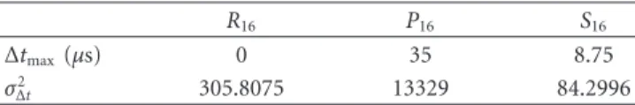
Optimal Convergence Rate. First we compare the conver-gence speeds of the SO-DCTS and FO-DCTS algorithms for the above structured networks assuming that the con-vergence rate is defined as ν = −log(α), and there is no Gaussian delay between nodes.Table 1 gives the numerical values of the optimal convergence rate for the SO-DCTS and FO-DCTS algorithms under theR16,P16, andS16topologies.
As expected, the SO-DCTS algorithm converges faster than the FO-DCTS algorithm in all three cases. Specifically, we see that the optimal convergence rate of the SO-DCTS algorithm is nearly twice as that of the FO-DCTS algorithm for all three types of networks.
Table1: Numerical results comparing convergence rates of FO-DCTS and SO-FO-DCTS algorithms inR16,P16,S16.
R16 P16 S16
αopt νopt αopt νopt αopt νopt
FO-DCTS Alg. 0.9267 0.0762 0.9808 0.0194 0.8824 0.1252 SO-DCTS Alg. 0.8634 0.1469 0.9623 0.0384 0.7895 0.2364
Table2: Asymptotic results for the SO-DCTS algorithm in struc-tured networks with Gaussian delay.
R16 P16 S16
Δtmax(μs) 0 35 8.75
σ2
Δt 305.8075 13329 84.2996
Convergence Properties of SO-DCTS Algorithm with Gaussian Delay. In our simulations of the SO-DCTS algorithm with Gaussian delay, we assumeTc+Lc/c=10 microseconds and
the optimal values ofεopt,SOandγopt,SOfrom (24). The
simu-lation results and the asymptotic mean square time synchro-nization errors for theR16,P16, andS16networks are shown
inFigure 5. For each network topology, the asymptotic mean square time synchronization errorσ2
Δtis calculated from (48).
It can be seen that as time index increases, mean square time synchronization error approaches the steady-state value when utilizing SO-DCTS algorithm with Gaussian delay. Additionally, we see that the SO-DCTS algorithm performs poorest in a path network where it has the largest value of
σ2
Δtand the slowest convergence speed. This is not surprising
since in such networks information flow from node 1 to node
nrequiresn−1 hops.
Table 2 summarizes the asymptotic results of the SO-DCTS algorithm for structured networks. As expected, the maximum asymptotic expectation of global time synchro-nization error forRnis 0 sinceRn is atime delay balanced
network. Furthermore, the SO-DCTS algorithm in Pn has
the largest Δtmax because of its highly unbalanced time
delay structure. It is worth mentioning that the SO-DCTS algorithm in star networks Sn has relatively small values
of Δtmax and σΔ2t. In fact, the SO-DCTS algorithm for a
star network can be seen as a type of centralized time synchronization algorithm in which a root node determines and propagates the average of local time information of all other nodes in the network.
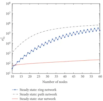
In Figure 6, we show the asymptotic value of σ2
Δt as a
function of the number of nodes in these structured net-works. It can be seen that when using the optimalεopt,SOand
γopt,SO, the asymptotic mean square time synchronization
error for a star network is nearly constant as the number of nodes increases. However,σ2
Δtis an increasing function of the
number of nodes for both path and ring networks.
(a) (b) (c)
Figure4: Structured networks: (a)R8, (b)P5, (c)S8.
101
102
103
104
105
106
107
σ
2 Δt
0 50 100 150
Iteration time index Steady state:R16
Simulation:R16
Steady state:P16
Simulation:P16
Steady state:S16
Simulation:S16 Figure 5: σ2
Δt as a function of the iteration time index for the SO-DCTS algorithm in structured networks (R16, P16, S16) with Gaussian delay.
is shown inFigure 7. We assume that the average distance between two nodes is 0.5 km.
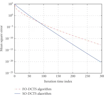
Figure 8shows the simulation results for the convergence rates of the FO-DCTS and SO-DCTS algorithms in random networks with 256 nodes whenη = 0.25 without Gaussian delay between network nodes. Specifically, we plot the mean square time synchronization error (defined as (1/n)δ(k)2).
In simulating random networks, we average results over 5000 network realizations. To obtain these results, we chose
εopt,FO for the FO-DCTS algorithm andεopt,SO and γopt,SO
for the SO-DCTS algorithm. In Figure 8, we observe that the optimal convergence rate of the SO-DCTS algorithm is faster than that of the FO-DCTS algorithm. In addition to the results shown here, we ran this simulation setup for various realizations of random networks, assuming bothn=256 and a smaller network withn = 16. Overall, the results show a similar trend, that is, the convergence rate of the SO-DCTS algorithm exceeds the FO-DCTS algorithm.
Figure 9 shows the simulation results when the SO-DCTS algorithm is implemented in a random network
101
102
103
104
105
106
107
108
σ
2 Δt
10 15 20 25 30 35 40 45 50 55 60 Number of nodes
Steady state: ring network Steady state: path network Steady state: star network
Figure6:σ2
Δtas a function of the number of nodes for the SO-DCTS algorithm in structured networks with Gaussian delay.
0 0.1 0.2 0.3 0.4 0.5 0.6 0.7 0.8 0.9 1
0 0.2 0.4 0.6 0.8 1
Figure7: Random network with 16 nodes used to obtain simula-tion results inFigure 9.
10−25
10−20
10−15
10−10
10−5
100
105
Me
an
sq
u
ar
e
er
ro
r
0 50 100 150 200 250 300
Iteration time index FO-DCTS algorithm
SO-DCTS algorithm
Figure8: Evolutions of the FO-DCTS and SO-DTS algorithms in random network with 256 nodes whenη=0.25 without Gaussian delay between network nodes.
−600
−400
−200 0 200 400 600
E
[
δi
(
k
)]
0 5 10 15 20 25 30
Iteration time index Δtmax
Figure9: Evolution of the average disagreement of the SO-DCTS algorithm in random network (seeFigure 7) with Gaussian delay between network nodes.
synchronization error persists between some pairs of nodes, that is, Δtmax = 26.4130 microseconds for this random
network. If we specify a thresholdΔtThto be greater than or
equal to thisΔtmax, we call this network as “average consensus achievable with tolerable synchronization error” as described inDefinition 1.
7. Conclusions
In this paper, we propose a novel discrete-time SO-DCTS algorithm to address the global timing synchronization problem in wireless sensor networks. We analyze several
important convergence characteristics of the SO-DCTS algorithm for directed and undirected networks. Addition-ally, we investigate the convergence region and optimal convergence rate of the SO-DCTS algorithm in undirected networks and claim that the optimal convergence rate of the SO-DCTS algorithm is superior to that of the FO-DCTS algorithm under an appropriate algorithm design. Furthermore, we investigate the asymptotic expectation and mean square synchronization error of the SO-DCTS algorithm when there is Gaussian delay between network nodes. In the future, we intend to investigate the effects of skew, link failure, and other practical conditions when utilizing the SO-DCTS algorithm in wireless sensor net-works.
Appendices
A. Convergence Region for SO-DCTS Algorithm
in Undirected Networks
Let us denote the pairs of eigenvalues ofHcorresponding to
λi(L) asλi(H) andλi(H), that is,
λi(H)=1
2
1−ελi(L) +1−ελi(L)
2
+ 4γελi(L)
,
λi(H)=1
2
1−ελi(L)−
1−ελi(L)
2
+ 4γελi(L)
.
(A.1)
Now, we examine the convergence region for the SO-DCTS algorithm based on conditions|λi(H)|<1, 1< i ≤
n, and|λi(H)|<1, 1< i≤n.
Case 1. Whenλi(H) andλi(H) are real values: in this case,
we have (1−ελi(L))2+ 4γελi(L)≥0, that is,
γ≥ −
1−ελi(L)
2
4ελi(L)
, 1< i≤n. (A.2)
In the following, we assume that 1 < i,i,i ≤ n unless otherwise stated.
(1) First, we consider the convergence region forλi(H).
After some manipulations, we can show that the convergence region is
γ <1, 0< ε < 3 λi(L)
∪
2−ελi(L)
ελi(L) < γ <
1, ε > 3 λi(L)
.
(A.3)
(2) Then, we consider the convergence region for
|λi(H)|<1 which is given as
γ <2−ελi(L) ελi(L)
, 0< ε < 3 λi(L)
Combining the convergence region forλi(H) andλi(H)
with (A.2), the convergence regionR1for this case is
R1=
Thus, we only need to examine the convergence region for
|λi(H)|. In order to satisfy the conditions, we have
Combining the above results, the convergence regionR2for
this case is
considering the increasing order of λi(L), the convergence
region for the SO-DCTS algorithm in (20) is obtained.
B. Solution for Minimization Problem
Here, we give a sketch solution to the spectral radius minimization problem in (23). Sinceλ2(L)≤ · · · ≤ λn(L),
the optimization problem is equivalent to minimize
max{|λ2(H)|,|λ2(H)|,|λn(H)|,|λn(H)|}. (B.1)
(1) First, we find the optimalγgivenεto minimize (B.1). Here, we consider four different cases depending on whether λ2(H),λ2(H),λn(H),λn(H) are real
values or complex values. After algebraic derivations, we can show that the minimum of (B.1) given
ε can be achieved when λ2(H) and λ2(H) are
real values and λn(H) and λn(H) are complex
values. Additionally, the following equation should be satisfied:
Then, we have the following relationship betweenε
andγ:
This work was supported in part by research grants from Thales Communications, Inc., Md, USA, and the National Science Foundation.
References
[1] D. Culler, D. Estrin, and M. Srivastava, “Overview of sensor networks,”Computer, vol. 37, no. 8, pp. 41–49, 2004. [2] S. Ganeriwal, R. Kumar, and M. B. Srivastava,
“Timing-sync protocol for sensor networks,” in Proceedings of the 1st International Conference on Embedded Networked Sensor Systems (SenSys ’03), pp. 138–149, Los Angeles, Calif, USA, November 2003.
[3] J. Elson, L. Girod, and D. Estrin, “Fine-grained network time synchronization using reference broadcasts,” in Proceedings of the 5th Symposium on Operating Systems Design and Implementation (OSDI ’02), pp. 147–163, Boston, Mass, USA, December 2002.
[4] M. Mar ´oti, B. Kusy, G. Simon, and ´A. L´edeczi, “The flooding time synchronization protocol,” inProceedings of the 2nd Inter-national Conference on Embedded Networked Sensor Systems (SenSys ’04), pp. 39–49, Baltimore, Md, USA, November 2004. [5] F. Sivrikaya and B. Yener, “Time synchronization in sensor networks: a survey,”IEEE Network, vol. 18, no. 4, pp. 45–50, 2004.
[6] A. Giridhar and P. R. Kumar, “Distributed clock synchro-nization over wireless networks: algorithms and analysis,” inProceedings of the 45th IEEE Conference on Decision and Control (CDC ’06), pp. 4915–4920, San Diego, Calif, USA, December 2006.
[8] L. Schenato and G. Gamba, “A distributed consensus protocol for clock synchronization in wireless sensor network,” in Proceedings of the 46th IEEE Conference on Decision and Control (CDC ’07), pp. 2289–2294, New Orleans, La, USA, December 2007.
[9] O. Simeone and U. Spagnolini, “Distributed time synchroniza-tion in wireless sensor networks with coupled discrete-time oscillators,” EURASIP Journal on Wireless Communications and Networking, vol. 2007, Article ID 57054, 13 pages, 2007. [10] H. G. Tanner, A. Jadbabaie, and G. J. Pappas, “Flocking in
fixed and switching networks,”IEEE Transactions on Automatic Control, vol. 52, no. 5, pp. 863–868, 2007.
[11] W. Ren and E. Atkins, “Second-order consensus protocols in multiple vehicle systems with local interactions,” in Proceed-ings of the AIAA Guidance, Navigation, and Control Conference (GN&C ’05), pp. 3689–3701, San Francisco, Calif, USA, August 2005.
[12] P. Lin, Y. Jia, J. Du, and S. Yuan, “Distributed consensus control for second-order agents with fixed topology and time-delay,” inProceedings of the 26th Chinese Control Conference (CCC ’07), pp. 577–581, Zhangjiajie, China, July-June 2007. [13] W. Ren, “Second-order consensus algorithm with extensions
to switching topologies and reference models,” inProceedings of the American Control Conference (ACC ’07), pp. 1431–1436, New York, NY, USA, July 2007.
[14] R. A. Horn and C. R. Johnson,Matrix Analysis, Cambridge University Press, Cambridge, UK, 1985.
[15] L. Xiao and S. Boyd, “Fast linear iterations for distributed averaging,” in Proceedings of the 42nd IEEE Conference on Decision and Control, vol. 5, pp. 4997–5002, Maui, Hawaii, USA, December 2003.
[16] C. D. Meyer, Matrix Analysis and Applied Linear Algebra, Society for Industrial and Applied Mathematics, Philadelphia, Pa, USA, 2001.
[17] R. Olfati-Saber and R. M. Murray, “Consensus problems in networks of agents with switching topology and time-delays,” IEEE Transactions on Automatic Control, vol. 49, no. 9, pp. 1520–1533, 2004.
[18] S. Kar and J. M. F. Moura, “Topology for global average consensus,” inProceedings of the 40th Asilomar Conference on Signals, Systems and Computers (ACSSC ’06), pp. 276–280, Pacific Grove, Calif, USA, October-November 2006.
[19] G. Xiong and S. Kishore, “Analysis of distributed consensus time synchronization with Gaussian delay over wireless sensor networks,” submitted toEURASIP Journal on Wireless Com-munications and Networking.