“Data Mining techniques differentiation between NPPLS and PLS”

(1)

A Monthly Double-Blind Peer Reviewed Refereed Open Access International Journal

International Journal in IT & Engineering

http://www.ijmr.net.in

email id- [email protected]

Page 1 “Data Mining techniques differentiation between NPPLS and PLS”

Manoj Kumar,Department of Computer Science Govt. College,Narnaul

09416259830

ABSTRACT:-

This paper compares two different predictive data-mining techniques (one linear technique, Partial Least Squares (PLS) and one nonlinear technique(NLPLS)) on two different and unique data sets: a collinear data set (called "the COL" data set in this paper) and a simulated data set (called "the Simulated" data in this paper). These data are unique, having a combination of the following characteristics: few predictor variables, many predictor variables, highly collinear variables, very redundant variables and presence of outliers. The natures of these data sets are explored and their unique qualities defined. This is called data pre-processing and preparation. To a large extent, this data processing helps the miner/analyst to make a choice of the predictive technique to apply. The big problem is how to reduce these variables to a minimal number that can completely predict the response variable. the Partial Least Squares (PLS, a supervised technique), and the Nonlinear Partial Least Squares (NLPLS), which uses some neural network functions to map nonlinearity into models, were applied to each of the data sets . Each technique has different methods of usage; these different methods were used on each data set first and the best method in each technique was noted and used for global comparison with other techniques for the same data set. The purpose of this is to identify the technique that performs best for a given type of data set and to use it directly instead of relying on the usual trial-and-error approach. When this process is effectively used, it will reduce the lead time in building models for predictions or forecasting for business planning. The work in this Research paper will also be helpful in identifying the very important predictive data-mining performance measurements or model evaluation criteria.

Keywords: PLS, NLPLS, COL, PDM

INTRODUCTION

(2)

International Journal in IT & Engineering

email id- [email protected]

Page 2 evaluating and making the best decisions based on records so as to create additional value and to prevent loss. The potential of data-mining for industrial managers has yet to be fully exploited

.

1. PREDICTIVE DATA MINING:

Hence, with the advent of improved and modified prediction techniques, there is a need for an analyst to know which tool performs best for a particular type of data set. In this paper, two prediction tools Partial Least Squares [PLS]; and Nonlinear Partial Least Squares [NLPLS]), are used on two uniquely different data sets to compare the predictive abilities of each of the techniques on these different data samples. The advantages and disadvantages of these techniques are discussed also. Hence, this study will be helpful to learners and experts alike as they choose the best approach to solving basic data-mining problems. This will help in reducing the lead time for getting the best prediction possible.

(3)

International Journal in IT & Engineering

email id- [email protected]

Page 3 proposed to serve as blueprints for how to organize the process of data collection, analysis, results dissemination and implementing and monitoring for improvements.

1.1 Partial Least The score vectors are the values of the data on the loading vectors p and q. Furthermore, a principle component-like analysis is done on the new scores to create loading vectors (p and q). Figure 2.4, an inferential design of PLS by Hines [15], is a representation of this. In contrast to principal component analysis (PCA), PLS focuses on explaining the correlation matrix between the inputs and outputs but PCA dwells on explaining the variances of the two variables. PCA is an unsupervised technique and PLS is supervised. This is because the PLS is concerned with the correlation between the input (x) and the output (y) while PCA is only concerned with the correlation between the input variables x. As can be seen in Figure 2.4, b would represent the linear mapping section between the t and u scores. The good point of PLS is that it brings out the maximum amount of covariance explained with the minimum number of components. The number of latent factors to model the regression model is chosen using the reduced eigenvectors.

The eigenvectors are equivalent to the singular values or the explained variation in the PC selection and are normally called the Malinowski’s reduced eigenvalue [6]. When the reduced eigenvalues are basically equal, they only account for noise.

Figure1.1 diagram of the PLS Inferential Design.

1.2 Non Linear Partial Least Squares (NLPLS)

This is shown diagrammatically in Figure 2.5, an inferential design of NLPLS by Hines [15]. It is just the same as the process explained above, with the major difference being that in the linear PLS method, the inner relationships are modeled using simple linear regression. The difference between PLS and the NLPLS models is that in NLPLS, the inner relationships are modeled using neural networks [20,19]. For each set of score vectors retained in the model, a Single Input Single Output (SISO) neural network is required [15]. These SISO networks usually contain only a few neurons arranged in a two-layered architecture. The number of SISO neural networks required for a given inferential NLPLS unit is equal to the number of components retained in the model and is significantly less than the number of parameters included in the model [16].

(4)

International Journal in IT & Engineering

email id- [email protected]

Page 4 Design.

PROCEDURE

The relationship check is made by plotting the inputs over the output of the raw data sets. The data is preprocessed by scaling or standardizing them (data preparation) to reduce the level of dispersion between the variables in the data set. The correlation coefficients of each of the various data sets are computed to verify more on the relationship between the input variables and the output variables. This is followed by finding the singular value decomposition of the data sets transforming them into principal components. This also will be helpful in checking the relationship between the variables in each data set. At this stage, the data sets are divided into two equal parts, setting the odd number data points as the "training set" and the even number data points as the "test validation data set." Now the train data for each data set is used for the model building. For each train data set, a predictive data mining technique is used to build a model, and the various methods of that technique are employed. For example, Multiple Linear Regression has three methods associated with it in this Research paper: the full model regression model, the stepwise regression method, and the model built selecting the best correlated variables to the output variables. This model is validated by using the test validation data set. Nine model adequacy criteria are used at this stage to measure the goodness of fit and adequacy of the prediction. The results are presented in tables. The results of the train sets are not presented in this study because they are not relevant. This is because only the performance of the model on the test data set or entirely different (confirmatory) data set is relevant. The model is expected to perform well when different data sets are applied to it. In this Research paper work, the unavailability of different but similar real-life data sets has limited this study to using only the test data set for the model validation. This is not a serious problem since this work is limited to model comparison and is not primarily concerned with the results after deployment of the model.

Finally, all the methods of all the techniques are compared (based on their results on each data set) using four very strong model adequacy criteria. The best result gives the best prediction technique or algorithm for that particular type of data set.

1. DATA INTRODUCTION:-

2.1 The COL Data Set Description and Preprocessing:-

The variables or attributes are simply designated as Variables 1 to 8, with variable 8 being the output variable and the rest being input variables. It was necessary to scale these to reduce the dispersion and bring all the variables to the same unit of measure. After scaling, the entire matrix now has a mean of 0 and standard deviation. The correlation coefficient matrix will reveal this relation better. It can be observed that all the variables are strongly correlated with each other. Indeed, they are almost perfectly correlated with each other and with the response variable. Therefore there is no nonlinear relationship between those PCs' scores plotted. This will further be revealed from the plot of inner scores matrix and outer score matrix of the Partial Least Square model and that of the Nonlinear Partial Least Squares.

2.2 The Simulated Data Set Description and Preprocessing:-

(5)

International Journal in IT & Engineering

email id- [email protected]

Page 5 reduce the degree of dispersion between the data points in the matrix. The data set was scaled once again to reduce this dispersion and give every point an equal opportunity of showing up in the matrix. Some of the variables showed good correlation with the output variable, but a great number of them didn't. After the scaled data were plotted, the cluster was now about zero (ranging from -2 to 2), with spikes showing outliers. The correlation coefficient matrix revealed a very weak correlation between the input and the output variables. One cannot see any presence of a nonlinear relationship, although the large data points may have hidden any trace of them.

2. THE STATISTICS OR CRITERIA USED IN THE COMPARISON:-

In this section, the entire nine criteria used to compare the various methods within each technique are briefly explained.

1. R-square (R2 or R-Sq) measures the percentage variability in the given data matrix accounted for by the built model (values from 0 to 1).

2. R-square Adjusted (R2 adj) gives a better estimation of the R2 because it is not particularly affected by outliers. While R-sq increases when a feature (input variable) is added, R2 adj only increases if the added feature has additional information added to the model. R2 adj values ranged from 0 to 1. 3. Mean Square Error (MSE). MSE measures the difference between the predicted test output and the

actual test outputs. The smaller the MSE, the better. Large MSE values mean poor prediction.

4. Root Mean Square Error (RMSE); this is just the MSE in the units of the original predicted data. It is calculated by finding the square root of MSE.

5. Mean Absolute Error (MAE); this quantity takes care of overestimation due to outliers.

6. Modified Coefficient of Efficiency (E-mod); the modified coefficient of efficiency gives information equivalent to the MAE (values from -1 to 1).

7. The Weight of the regression models (norm); this value calculates the weights of the regression coefficients.

8. Condition number of the predictor matrix (CN); this quantity, designated as CN here, gives a measure of the stability of the model built. High condition numbers (> 100) show that the problem is ill-conditioned and hence cannot give consistent or stable results.

9. Number of features or variables used (N). The objective of every builder is to make use of the smallest amount of resources to achieve the desired result, as per Occam's Razor. Since data collection and analysis are expensive, fewer features (variables) take less energy and resources to deal with.

(6)

International Journal in IT & Engineering

email id- [email protected]

Page 6 model was trained. If a model performed very well in the training set and could not perform satisfactorily in the test validation data set or new data sets, then its predictive ability is suspect and cannot be used for prediction. Hence, the results of the predictions of the training sets' output were not presented in this analysis because the performances of the models in the test validation data set are of more significance to this study. Only the predictions of the response variables of the test validation data sets were used for the model comparison.

3. COL DATA SET ANALYSIS:-

The description of the COL data shows that the variables were almost perfectly correlated with each other; therefore this data set was divided in a unique way to avoid the replication of the train data set on the test data set. Dividing this data as before would mean having the train data set and test data set is almost the same, so in this case, the data were divided into blocks of 200s. The odd blocks were the training set, and the even blocks were the test set (this is different from the earlier division into odd numbers as training set and even numbers as test set). In this division, care was taken to make sure the training set covered the entire data matrix.

4.1 Partial Least Squares (PLS) on COL data:-

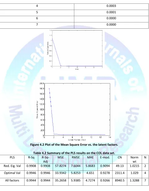
In the COL data analysis, three models of the PLS were built. Using Malinowski’s eigenvalues, (Table 4.1), the plot of the reduced eigenvalues against the index shows that two factors looked significant (Figure 4.1). Using the iterative method, the minimum MSE gave four optimal numbers of factors (Figure 4.2). Finally a model was made using all the factors. The result of these various models is shown in the Summary Table (Table 4.2).

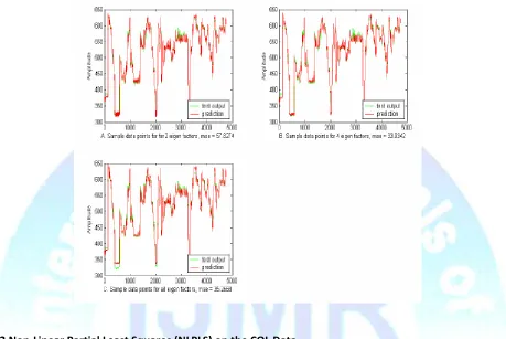
As can be seen in Table 4.2, the best model is the optimal eigenvalue model (four factors). From the reduced eigenvalues Table 4.1, the fifth factor to the seventh factor seemed to have reduced eigenvalues that were equivalent and could be classified as noise. The solution of the optimal factors (4 factors) and that of the model built with all the factors looked almost the same in terms of the R.Sq. the R2 adj, the RMSE, the MAE and the modified coefficient of efficiency. Their condition numbers CN were above 2,000. The model built with only two factors had a good condition number (49), and the R.Sq and R2 adj were not bad, but the MSE was relatively high (57.8). Figure 4.3 shows the predictions of the test output data with two, four and all of

the seven factors. Figure 4.4 shows the output scores plotted over the input scores (predicted and test response). This plot shows that the model is a linear one. The data itself looked linear and the model represents that. The generalization of the linear pattern was good. Perhaps NLPLS after training will copy the nonlinearity or over-fit the data.

Figure 4.1 Plot of the reduced eigenvalues vs. the index.

Table 4.1 Malinowski's reduced eigenvalues for the COL data.

Reduced Eigenvalues

1 1.0920

2 0.0206

(7)

International Journal in IT & Engineering

email id- [email protected]

Page 7 Figure 4.2 Plot of the Mean Square Error vs. the latent factors.

Table 4.2 Summary of the PLS results on the COL data set. PLS R-Sq R-Sq-

Adj

MSE RMSE MAE E-mod. CN Norm wt

N

Red. Eig. Val 0.9908 0.9908 57.8274 7.6044 5.8683 0.9094 49.13 1.0215 2

Optimal Val 0.9946 0.9946 33.9342 5.8253 4.651 0.9278 2311.4 1.029 4

All factors 0.9944 0.9944 35.2658 5.9385 4.7274 0.9266 8940.5 1.3288 7

4 0.0003

5 0.0001

6 0.0000

(8)

International Journal in IT & Engineering

email id- [email protected]

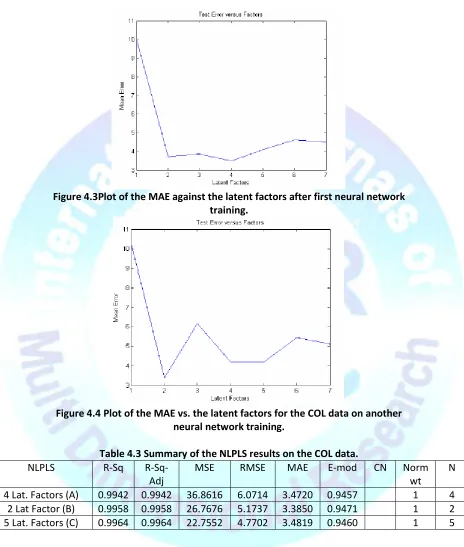
Page 8 4.2 Non-Linear Partial Least Squares (NLPLS) on the COL Data

(9)

International Journal in IT & Engineering

email id- [email protected]

Page 9 Figure 4.3Plot of the MAE against the latent factors after first neural network

training.

Figure 4.4 Plot of the MAE vs. the latent factors for the COL data on another neural network training.

Table 4.3 Summary of the NLPLS results on the COL data.

NLPLS R-Sq

R-Sq-Adj

MSE RMSE MAE E-mod CN Norm

wt

N

(10)

International Journal in IT & Engineering

email id- [email protected]

Page 10 Figure 4.5 Output scores over the input scores (predicted and test response).

4.3 SIMULATED DATA SET ANALYSIS

The Simulated data set was introduced in this section . This data set has a total of 44 variables. The response variable is the 38th variable (this occupied the 38th column before data preprocessing).

4.4 Partial Least Squares on Simulated Data Set

Four models were built with PLS on the simulated data set. Using Malinowski's reduced eigenvalues plot (Figure 4.8), the minimum reduced Eigen factor is not obvious. Factor numbers 3 and 5 were used to build models and the results are given in table 4.4 (first two results in the table). Then the iterative method (generalization) was used to find the optimal number of factors to get a minimum MSE. Figure 4.9 was used to find the optimal number of factors. Looking at the plot, at point 8 latent factors, the line touched the x-axis and ran parallel to that axis. Hence factors 8 and 43 were used to build the model. The summary of the PLS results is shown in Table 4.4. From Table 4.4, the best solution using PLS was the model built with the optimal number of factors (8) from the iterative (generalization) method. It has the best MSE compared to the others, and the condition number was below 100. Figure 4.10 shows the plot of the internal scores vs. the predicted internal scores.

GENERAL RESULTS AND CONCLUSION:-

(11)

International Journal in IT & Engineering

email id- [email protected]

Page 11 best model. Models with fewer variables, factors or PCs were favored over others. MAE is especially useful in resolving the problem MSE has with outliers. MSE is not regarded as a better measuring criterion than MAE.

SUMMARY OF THE RESULTS OF PDM TECHNIQUES:-

This section gives the summary results of the various techniques used in this Research paper work and how they performed in each type of data set. It also covers the advantages of each technique over the other.

COL Data Results Summary for All the Techniques:-

The COL is a highly ill-conditioned data set. The best model for this data set is the Partial Least Squares (PLS), built with two factors. Among all the models that are below the condition number of 100, it has the best MSE and MAE. The second best is the PCR model with only two PCs. It has MSE lower than the group that survived the condition number elimination. Again, the NLPLS gave the best model if MSE is the only criterion for comparison. It can be seen that the solution is not stable. It has three optimal solutions. Each time the model was retrained, a new optimal solution is obtained. It mapped nonlinearity into the model and hence can only be useful if a nonlinear model is being considered. Simulated Data Results Summary for All the Techniques:-

The Simulated data set with many input variables has the PLS with optimal factors as the best model for prediction. This is followed by the PCR model with 29 PCs. Both models gave the same measurements, but the PLS came up better by the number of factors used in the model. It used only 8 out of 43 factors for its prediction. The NLPLS also mapped nonlinearity into the model. This is not good because the relationship of the regression is a linear one.

CONCLUSION

In conclusion, in the course of this work, the various data preprocessing techniques were used to process the two data sets. Some of the data sets were seen to have unique features; an example is the COL data set, which is very collinear. PLS generally performed better than all the other four techniques in building linear models. It dealt with the co linearity in the COL data and gave the simplest model that made the best predictions. The PLS also reduced the dimensionality of the data. The study shows that supervised techniques demonstrated a better predictive ability than unsupervised techniques. It can be seen that in MLR and PCR, the correlation-based models which were supervised techniques performed reasonably better than most models where variables and PCs were randomly selected to build the model. The variables that added valuable information to the prediction models were variables that had correlation with the output being predicted.PLS with two factors. From the analysis, it can be seen that the condition number of any data matrix has a direct relation to the number of statistically significant variables in the model. Based on the results from the Summary Tables and the discussion so far on the predictive linear modeling techniques.

RECOMMENDATIONS FOR FUTURE WORK:-

(12)

International Journal in IT & Engineering

email id- [email protected]

Page 12 vector machines. Another area of data-mining that has been and will continue to be a fertile ground for researchers is the area of data acquisition and storage. The ability to correctly acquire, clean, and store data sets for subsequent mining is no small task. A lot of work is going on in this area to improve on what is obtainable today. There are many commercial software packages produced to solve some of these problems but most are uniquely made to solve particular types of problem. It would be desirable to have mining tools that can switch to multiple techniques and support multiple outcomes. Current data-mining tools operate on structured data but most of the data in the field are unstructured. Since large amount of data are acquired, for example in the World Wide Web, there should be tools that would manage and mine data from this source, a tool that can handle dynamic data, sparse data, incomplete or uncertain data. The dream looks very tall but given the time and energy invested in this field and the results which are produced, it will not be long to get to the development of such software.

REFERENCES:-

1. Lyman, P., and Hal R. Varian, "How much storage is enough?" Storage, 1:4 (2003).

2. Way, Jay, and E. A. Smith,"Evolution of Synthetic Aperture Radar Systems and Their Progression to the EOS SAR," IEEE Trans. Geoscience and Remote Sensing, 29:6 (1991), pp. 962-985.

3. Usama, M. Fayyad, "Data-Mining and Knowledge Discovery: Making Sense Out of Data," Microsoft Research IEEE Expert, 11:5. (1996), pp. 20-25.

4. Berson, A., K. Thearling, and J. Stephen, Building Data Mining Applications for CRM, USA, McGraw-Hill (1999).

5. Malinowski, E. R., "Determination of the Number of Factors and The Experimental Error in a Data Matrix." Anal. Chem. 49 (1977), pp. 612-617.

6. Sharma, K. Sanjay, et al., "A Covariance-Based Nonlinear Partial Least Squares Algorithm," Intelligent Systems and Control Research Group (2004).

7. Giudici, P., Applied Data-Mining: Statistical Methods for Business and Industry. West Sussex, England: John Wiley and Sons (2003).

8. Berry, M. J. A., and G. S. Linoff, Mastering Data Mining. New York: Wiley (2000).

9. Han, J., and M. Kamber, Data Mining: Concepts and Techniques. New York: Morgan Kaufman (2000). 10. Pregibon, D., "Data Mining," Statistical Computing and Graphics, pp. 7-8. (1997).

11. Usama, M. Fayyad, et al., Advances in Knowledge Discovery and Data Mining. Cambridge, Mass.: MIT Press (1996).