TH E D Y N A M IC R E SP O N SE OF A N
IM PA C T IN G D R IV E N BEAM :
E X P E R IM E N T S A N D M ATH EM A TIC AL
M ODEL
George Karpodinis
Supervisor: Professor S. R. Bishop
Thesis submitted in partial fulfilment of the requirements
for the degree of
Doctor of Philosophy in Nonlinear Dynamics
Centre for Nonlinear Dynamics and its Applications
University College London
ProQuest Number: U643564
All rights reserved
INFORMATION TO ALL USERS
The quality of this reproduction is dependent upon the quality of the copy submitted.
In the unlikely event that the author did not send a complete manuscript and there are missing pages, these will be noted. Also, if material had to be removed,
a note will indicate the deletion.
uest.
ProQuest U643564
Published by ProQuest LLC(2016). Copyright of the Dissertation is held by the Author.
All rights reserved.
This work is protected against unauthorized copying under Title 17, United States Code. Microform Edition © ProQuest LLC.
ProQuest LLC
789 East Eisenhower Parkway P.O. Box 1346
A bstract
Systems consisting of vibrating components th a t repeatedly impact with rigid boundaries are in the heart of engineering. The aim of this research is to improve our understanding of such vihro-impact systems and thus to enable more accurate monitoring, interpretation and modelling of their behaviour.
We use a mechanical impacting oscillator as our source of experimental data. An impact load cell is used to measure the forces exerted upon impact. These data are analysed to assess the suitability of an instantaneous impact assumption for the impacts. The problem is quantified and the suitability of the model is proved. The single degree of freedom model, combined with an instantaneous impact rule, is then used to compare and verify our experimentally obtained results.
Using thresholded measurements from the im pact load cell, we show th at the correlation dimension can be estimated. Using interspike intervals from the vibro- impacting motion, we successfully reconstruct the dynamics of the system for different kinds of periodic behaviour. By simulating the d ata acquisition process, we also show th a t the results obtained by thresholding the measurements are qualitatively similar to results obtained in ‘noisy’ environments.
A way to remotely extract the same information from the vibro-impact sys tem is presented. We investigate whether the sound of the impacts carries enough information to reconstruct the dynamics. We show th a t this is possible by re constructing two types of behaviour. The results show great similarity to those obtained from the impulse spike data.
A cknow ledgem ents
I would like to thank my supervisor, Professor Steven R. Bishop, for his guidance, support and tru st throughout the period of this work. He has deeply influenced my interest for research and my knowledge of dynamics.
Also thanks to David Wagg for initiating me to the experimental procedures, to Ching Luan Lau and Johan Iskandar Hasan for providing some of the sound recordings used for the work presented in chapter 5, to Simon Justin for his support in and out of college, and to Evaki for helping with the printing.
Many thanks to my colleagues in the Wolfson dynamics laboratory at UCL for providing a nice environment to work in, and especially to Giovanni Santoboni for his friendship.
C O N T E N T S
C on ten ts
A b s tr a c t... 3
A cknow ledgem ents... 4
C o n te n ts ... 5
List of F ig u res... 9
List of T a b l e s ... 15
1 In tro d u ctio n 16 1.1 Evolution of nonlinear dynamics and chaos t h e o r y ... 17
1.2 Vibro-impact sy ste m s... 19
1.2.1 Vibro-impact systems in e n g in e e r in g ... 19
1.2.2 Modelling of vibro-impacting ... 21
1.3 Relevant research in nonlinear d y n a m i c s ... 25
1.3.1 Impact map and Grazing b ifu rcatio n s... 26
1.3.2 Interspike in te r v a ls ... 27
1.4 Motivation and o b je c tiv e s ... 29
2 M od ellin g sin gle degree o f freedom vib ro-im p act sy stem s 31 2 . 1 Oscillatory m o t i o n ... 32
2.1.1 Equation of m o tio n ... 32
2.1 .2 Analytic solutions for an underdamped s y s te m ... 32
2.2 Time history and phase p o r t r a i t s ... 34
2.3 Vibro-impacting m o t i o n ... 35
2.3.1 Instantaneous im p a c t... 35
C O N T E N T S 6
2.4 Solution methods for the combined m o tio n ... 37
2.4.1 Semi-analytical m e th o d ... 38
2.4.2 Numerical m e t h o d ... 40
2.5 System-specific p a ra m e te rs... 42
3 E x tra ctin g in form ation from ex p erim en ta l tim e series 46 3.1 Fundamental embedding t h e o r y ... 47
3.1.1 Delay c o o rd in a te s... 48
3.1.2 An example of delay coordinates re c o n s tr u c tio n ... 49
3.2 Interspike i n t e r v a ls ... 51
3.2.1 The integrate-and-fire m o d e l... 52
3.2.2 The threshold-crossing m o d e l ... 55
4 E x p erim en ta l an alysis th rou gh im p u lse spike recordings 61 4.1 Experimental s e t u p ... 62
4.2 Recording of d a t a ... 63
4.2.1 Sampling r a t e ... 65
4.2.2 T h r e s h o ld in g ... 6 6 4.3 Information from impulse s p ik e s ... 67
4.3.1 Frequency dependence of impact force ... 67
4.3.2 Duration of impacts ... 69
4.3.3 Multiple impact s p ik e s ... 72
4.3.4 Measurement of impact force ... 73
4.4 Information from interspike i n t e r v a l s ... 75
4.4.1 Spike t r a i n s ... 76
4.4.2 Correlation d im e n s io n ... 77
4.4.3 Delay Reconstruction - Periodicity ... 79
4.4.4 Simulation of the data acquisition p r o c e s s ... 84
C O N T E N T S
5.2 Recording and processing of sound f i l e s ... 93
5.3 R e s u lts ... 96
5.3.1 Periodic m o tio n ... 96
5.3.2 G r a z i n g ... 97
5.4 Comparison with the impulse spike m e th o d ... 100
6 C ontrol o f th e vib ro-im p act sy stem 102 6.1 In tro d u c tio n ...102
6.1.1 Fundamental theory of control m e th o d s ... 103
6.1.2 The OGY a l g o r it h m ...105
6.1.3 Other control te c h n iq u e s ... 107
6.2 Pyragas’s m e th o d ... 109
6.3 Periodic orbits in the vibro-impact s y s t e m ... I l l 6.4 Problem specific c o n s id e ra tio n s ... 112
6.5 R e s u lts ... 114
6.5.1 Stabilisation of periodic o r b i t s ...114
6.5.2 Effect of the control p a r a m e te rs ... 118
6 . 6 Impact re g u la tio n ... 120
6.7 Migration between o r b it s ... 122
6 . 8 Performance considerations ...123
7 C on clusions 127 Further improvements and future w o r k ... 130
A E xp erim en tal setu p 133 A .l General a rra n g e m e n t... 133
A.2 The im pact load c e l l ... 133
A.3 Forcing and data a c q u isitio n ... 136
A.4 D ata acquisition softw are... 138
C O N T E N T S 8
B.2 Free o s c illa tio n ... 142 B.3 Solution for a cantilever b e a m ... 143
C C on ten ts o f cover C D 146
L I S T OF F IG U R E S
List o f Figures
1 .1 The Lorenz attra cto r... 18 1 .2 a) A SDOF model for an impact oscillator, b) Schematic diagram
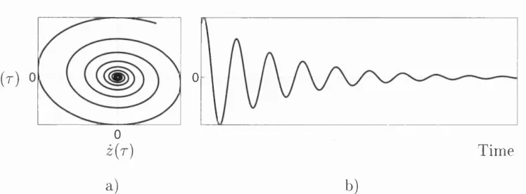
of the horizontal forces acting on mass m, shown in a )... 2 1 2.1 Evolution of an initial condition of a free, underdam ped oscillator,
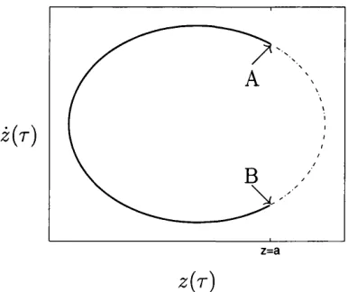
a) Phase space plot, b) Time history plot. The gridlines at zero indicate the equilibrium position... 34 2.2 Phase portrait of a periodic orbit with one impact per forcing cycle
(solid line) and the same orbit without impacting (dashed line). Motion is clockwise. A, B are solutions of z { t ) = a... 39
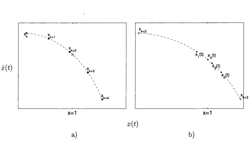
2.3 a) Iteration steps, b) Successive impact approximations, a: = 1 is the position of the impact stop ... 41 2.4 Power spectrum of an unforced non-impacting oscillation... 43 2.5 Deflection A, at the free end of a cantilever beam, upon action of a
static force, P... 43 3.1 a) a7!/-projection of the Rossler attractor. Rest of flgures are recon
structions with a different lag, I. h) I = 1, c) I = 10, d) I = 15, e) / = 20, f) Z = 24... 50 3.2 Graphical representation of a typical spike train. Vertical lines cor
respond to flring tim es... 52 3.3 a) xy-projection of the Rossler attractor, b), c): reconstructions
L I S T O F FI G U R E S 10
3.4 Reconstructions of the Rossler attractor using interspike intervals generated by the integrate-and-fire model. From left to right the value for C is 2 0, 30, 40, 50 and 60... 54 3.5 Reconstructions of the Rossler attracto r using interspike intervals
generated by the integrate-and-fire model. From left to right the value for I is 2, 4, 6 and 8. C = 40... 54 3.6 a) Poincaré section created by a period-2 orbit a.t x = 2. b) Poincaré
section created by a chaotic orbit at a: = 0... 55 3.7 Example of identification of periodic behaviour by means of inter
spike intervals, produced by a threshold-crossing m ethod... 57 3.8 a) A period- 1 orbit and the surface dX x = 1, used as a threshold for
the firing times, b) Delay plot of the interspike intervals produced by crossing of the threshold at a; = 1 from the period- 1 orbit shown in a ) ... 59 4.1 A schematic diagram of the experimental apparatus... 62 4.2 Time series of a vibro-impact motion showing response of impact
load cell, 6(r), as strain in volts using a sample rate of 60000 sam ples/second. (a) 5000 samples (b) 120 sample close up of impulse spike, individual samples shown as diamonds. (Figure produced by D.J. Wagg) ... 64 4.3 Time series of a vibro-impact motion showing the displacement of
the beam top (dotted) and response at the im pact load cell (solid). (Figure produced by D.J. W ag g )... 67 4.4 Time series data recorded from impact load cell (a) /= 2 1 .5 Hz, (b)
/= 2 2 .5 Hz, (c) f= 2 S .l Hz, (d) /= 2 4 .0 Hz. (Figure produced by D.J. Wagg) ... 6 8 4.5 Variation of the time of contact measure, fin, with forcing frequency,
/ , from experimental d a ta ... 71 4.6 a) Contact time, Tc, v s interspike interval, I for the d ata shown in
L I S T O F F I G U R E S 11
4.7 Variation of the average recorded peak force with forcing frequency. Values were retrieved from time series sampled at 50000 samples/sec. 74 4.8 Detail of a typical spike train, recorded from the strain gauge. / =
20.1 Hz ... 77 4.9 Interspike interval sequences for (a) / = 22.1 Hz (b) / = 20.1 Hz.
(c), (e) Correlation dimension for d ata in (a), (d), (f) Correlation dimension for data in (b). Legend: diamonds: m = 1, crosses: m = 2, boxes: m = 3. (Figure produced by D.J. W a g g ) ... 78 4.10 Experimental interspike interval delay plot: a) / = 22.1 Hz, b)
/ = 20.1 Hz... 80 4.11 Histogram of probability density of interspike intervals, p{I): a)
/ = 22.1 Hz, b) / = 20.1 Hz... 81 4.12 Numerically generated histogram of probability density of interspike
interval data for chaotic motion. (Figure produced by D.J. Wagg) . 83 4.13 Time series, recorded from the strain gauge. / = 21.5 Hz, sampling
rate=50000 samples/sec... 84 4.14 The effects of the data acquisition process on experimental results.
Numerical signal; (a) with added noise; (b) with noise and missed spikes; (c) with noise, missed and spurious spikes, (d) experimental d a ta ... 85 4.15 a) Schematic diagram of a spike train. The horizontal line shows
time and the thin vertical lines denote impact times. The upper part is the period- 1 train, whereas the lower part contains a spurious impact denoted by the thick vertical line, b) ISI delay plot of the spike trains in a). The filled circle is the outcome of the period-1 train. The open circles appear with the introduction of the spurious spike... 8 6 4.16 Phase portraits produced numerically at / = 22.1 Hz, with different
L I S T O F F IG U R E S 12
4.17 Delay plots of the interspike intervals for the phase portraits shown in figure 4.16. From left to right, the noise percentage is 0%, 0.247%, 0.476% and 0.960% respectively... 8 8 4.18 Probability distributions of interspike intervals against noise level.
Produced numerically for a) / = 2 2 . 1 Hz, b) / = 20.1 Hz... 89 4.19 Comparison of p(I) histograms for / = 20.1 Hz: a) experimental,
b) numerical with noise level 0.713%... 91 5.1 A schematic diagram of the experimental apparatus...93 5.2 Top plot: sample of sound recorded at 22050 Hz. The plot contains
4410 points. Bottom plot: same plot converted to a sampling rate of 8000 Hz. Contains 1600 points... 94 5.3 Circled peaks correspond to impacts identified by the computer pro
gram. Top plot: peaks correctly identified as impacts. Bottom plot: a badly recorded impact is missed by the computer program at 21.38 sec... 96 5.4 Interspike intervals for / = 23.81 Hz. a) Delay plot, b) Probability
distribution of I values... 97 5.5 Part of a sound recording from grazing behaviour. Impacting alter
nated with long intervals of non-impacting motion. The distance between gridlines on the time axes corresponds to three complete cycles of the forcing... 98 5.6 Interspike intervals for / = 21.55 Hz. a) Delay plot, b) Probability
distribution of I values... 99 6 . 1 The transition to chaos of the logistic map {xi+i = C — x ] )... 103 6 . 2 Diagram of the periodicity of the impacting oscillator. Estim ated
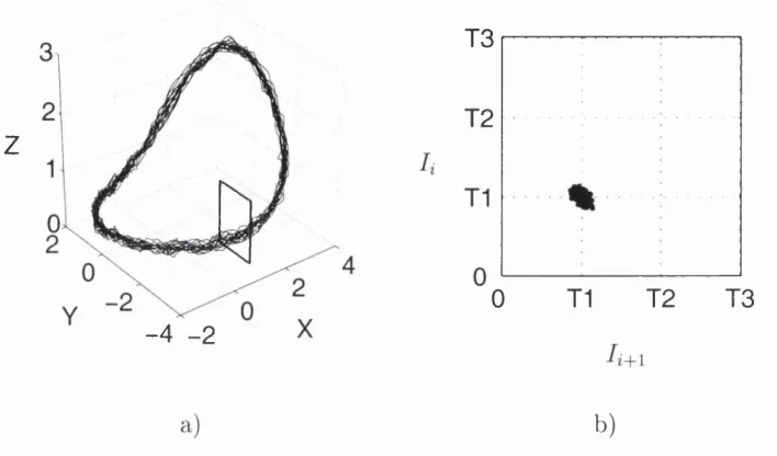
from numerical d a ta ... I l l 6.3 Phase portrait of the vibro-impact system at / = 20.3355 Hz. Mo
L I S T O F F IG U R E S 13
6.4 Phase portrait of a stabilised p erio d (l,l) orbit (solid black line). Control parameters: K = 0.15, Fq = 0.1. The light grey trace is
the regime covered by the chaotic trajectories...114 6.5 Evolution of orbit after activation of control, targeting a
period-1 orbit. Control starts at the 2 0 0 0 0 0th iterate. Top: speed, y{t). Middle: control perturbation, F (t). Bottom: time delay, r . Control parameters: F = 0.15, Fq = 0.1... 115 6 . 6 Phase portrait of a stabilised period(l,2) orbit (solid black line).
Control parameters: K = 0.15, Fq = 0.1. The light grey trace is the regime covered by the chaotic trajectories...116 6.7 Evolution of orbit after activation of control, targeting a
period-2 orbit. Control starts at the 200000th iterate. Top: speed, y{t). Middle: control perturbation, F{t). Bottom: tim e delay, r . Control parameters: F = 0.15, Fq = 0.1... 117 6 . 8 Phase portrait of an unsuccessful attem pt to stabilise a p erio d (l,l)
orbit. Control parameters: K = 0.01, Fq = 0.1...119 6.9 Phase portrait of an unsuccessful attem pt to stabilise a p erio d (l,l)
orbit. Control parameters: K = 0.45, Fq = 0.1...119 6.10 Phase portrait of a stabilised period(2,4) orbit (solid black line).
Control parameters: K = 0.05, Fq = 0.1. The light grey trace is the regime covered by the chaotic trajectories...1 2 0 6.11 Superimposed phase portraits of controlled orbits: Blue: p erio d (l,l).
Red: period(l,2). Black: period(2,4)...121 6 . 1 2 Superimposed y(t) histories of controlled orbits: Blue: p erio d (l,l).
Red: period(l,2). Black: period(2,4)...121 6.13 Regulation of impacts using control... 122 6.14 Migration between different periodic orbits. 200000-230000 iter
ates: p erio d (l,l); 230000-260000 iterates: period(l,2); 260000- 300000 iterates: p erio d (l,l). Top: speed, y{t). Middle: control perturbation, F{t). Bottom: time delay, r . Control parameters:
L I S T O F F IG U R E S 14
6.15 Evolution of orbit after activation of control, targeting a period-2 orbit. Control starts at the 200000th iterate. Top: speed, y{t). Bot tom: control perturbation F{t). Control parameters: K = 0.015,
Fq = 0.1... 125 6.16 Controlled period- 1 (solid) and period-2 (dashed) orbits of the Rossler
system...126 A .l Schematic representation of the experimental setup... 134 A. 2 Schematic representation of the impact load cell. All dimensions
are in mm. (Figure produced by D.J. W a g g ) ...135 A.3 Impact load cell positioned in cantilever beam experimental appa
ratu s... 136 A.4 Schematic representation of the connections between the personal
computer and the instrum entation... 137 B .l a) Uniform beam with distributed load q{x). b) Differential element
of the beam in a )...141 B.2 Shapes of the first three modes of vibration of a uniform cantilever
L I S T O F T A B L E S 15
List o f Tables
2 . 1 Summary of the parameters used in the modelling of the vibro- impact system ... 45
6 . 1 Summary of perturbation magnitudes for controlled period(1,1) and period(l,2) orbits. Values in parentheses refer to percentage of the
y(t) am plitude...118 B .l Summary of the first three solutions of (B.16) and the corresponding
C H A P T E R 1. I N T R O D U C T I O N 16
C hapter 1
In trod u ction
In the recent years there has been a great interest in the field of nonlinear dy namics. This interest is fuelled mainly by two factors: the frequent occurrence of nonlinear dynamical systems in virtually every field of science and engineer ing and the increasing availability of computing power, which makes the solution of complicated problems feasible and inexpensive. Furthermore, as scientific and engineering problems become more complex, linear theory reaches its limits and nonlinearity must be dealt with, in order to obtain working solutions.
In an engineering context, nonlinear response can usually be attributed to the stiffness an d /o r damping properties of the dynamical system, since inertia prop erties are in most cases linear. Nonlinear systems may still be smooth, if the dynamical equations can be differentiated with respect to time. Meanwhile, a large class of systems often encountered in engineering is impact oscillators or
vibro-impact systems. These terms are used to describe systems whose compo
C H A P T E R 1. I N T R O D U C T I O N 17
Im pact oscillators have a key role in the field of dynamics. Their behaviour resembles th a t of many systems in physics, biology and engineering. Motivation for this work arises from an interest to better understand the dynamics of such systems, as it is captured by experimental measurements. A complete framework of analysis would be beneficial in a vast number of problems. Furthermore, accurate modelling of their behaviour would assist in prediction of their response. The application of this in the design of structures, engines or mechanical manipulators in the manufacturing industry is of great interest.
1.1
E volution o f nonlinear dynam ics and chaos
th eory
In the Newtonian view of mechanics, dynamical systems are deterministic i.e. the future evolution of every system is completely and accurately determined by well-defined equations of motion and knowledge of its present state. Laplace also believed in such determinism. He is attributed with saying th a t given precise knowledge of the initial conditions, it should be possible to predict the future of the universe.
This is true in fact for any deterministic system. However, Poincaré (1892) studied the three-body problem in celestial mechanics and established th a t un predictable long-term behaviour may indeed be exhibited by totally deterministic systems. This is because many systems depend sensitively on their initial con ditions and therefore small inaccuracies in the initial conditions result in large differences in the long-term behaviour.
After Poincaré, Birkhoff continued working in the same field, taking Poincaré’s work a bit further (Birkhoff 1927; Birkhoff 1932; Birkhoff 1935). Many other re searchers since then, have studied certain features of dynamical systems, or solu tions to particular differential equations (Duffing 1918; van der Pol 1927; Andronov & V itt 1930; Andronov & Leontovich 1939; Cartwright 1948).
C H A P T E R 1. I N T R O D U C T I O N 18
30
Z
20
-1 0
-2 0
-1 0
X
F ig u r e 1.1: T he Lorenz a ttra c to r.
begun to ap pear. This was when Lorenz devised a sim ple m eteorological model
for the purpose of w eather forecasting. T he m odel consisted of three first-order
ord inary differential equations (O DEs) w ith three variables: the direction of move
m ent, the horizontal and the vertical d istrib u tio n of tem p eratu re. B ehaviour was
determ ined by the values of three param eters.
In his fam ous p ap er (Lorenz 1963), he described th e behaviour of his dynam ical
system . Lorenz was th e first to notice th e exponential divergence of nearby tr a
jectories, resulting in unpredictability. T his type of behaviour i.e. un predictable
long-term evolution in determ inistic nonlinear dynam ical system s, is now called
chaos. Evidently, nonlinear dynam ics and chaos theory are very much related.
T he Lorenz system is now known to behave chaotically a t certain values of its
p aram eters. T he Lorenz a ttra c to r (see figure 1.1) has since becom e a sym bol of
chaos theory.
T h e m ain consequence of chaos is th a t given im perfect knowledge — which is
practically always th e case — the horizon of p red ictab ility in a determ inistic system
becom es finite and in m any cases quite short, due to th e exponential grow th of
errors.
C H A P T E R 1. I N T R O D U C T I O N 19
phase space of forced oscillators, experimenting with electronic circuits. The study of nonlinear and chaotic phenomena flourished during the following two decades. One of the most influential discoveries was th at there are universal, scale invari ant properties in systems’ transition into chaos (Feigenbaum 1978, 1980). These properties have also been verifled experimentally (Libchaber et al. 1983).
1.2
V ibro-im pact system s
1.2.1 V ibro-im pact system s in engineering
Impacting is the single most im portant feature of vibro-impact systems dictating their design. Most design considerations will be towards minimising unwanted side effects of the impact, such as noise, components wear, aperiodic and large am plitude vibrations.
In mechanical engineering, expressions of such problems can usually be ob served in machinery with clearance between components, such as gears and bear ings. Numerous researchers (Pfeiffer & Kunert 1990; Kahram an & Singh 1991; Neilson & Gonsalves 1993; Wiercigroch 1994; Padm anabhan et al 1995) have studied such systems in the past, aiming both to model the systems’ behaviour and to provide solutions to problems such as gear rattle or wear of machinery.
Wood & Byrne (1981, 1982) studied random repeated im pacting processes. Their work focused on industrial applications with an emphasis on machine noise reduction. They also mentioned evidence of seemingly random behaviour in sinu soidally forced systems.
O ther problems encountered in mechanical engineering literature are the dy namics of rail vehicles and wheels (Meijaard & de Pater 1988; Knudsen et al 1992; Hassard 2000) and the dynamics of print hammers (Hendriks 1984; Tung & Shaw 1988).
C H A P T E R 1. I N T R O D U C T I O N 20
(Eisinger 1980; Abd-Rabbo & Weaver 1986; Chen 1989; Fisher et al, 1989; Au- Yang et al. 1991; Yetisir et al. 1998) because of the noise levels it produces and the potential for severe damage when vibrations become strong.
Problems of similar nature also arise in offshore engineering. Moored or teth ered sea vessels are known (Lean 1971; Rainey 1978; Thompson et al. 1984; Papoulias & Bernitsas 1988; Sharma et al. 1988; Aghamohammadi & Thompson 1990; Jin & Hu 1998) in many cases to undergo nonlinear or chaotic motion un der the combined action of the sea waves, which act as external forcing and the fenders, acting as movements constraints.
Earthquake excitation of high rise buildings th a t are very close together may also result in vibro-impacting. This phenomenon is known as ‘pounding’ and is mainly observed in earthquake-prone cities with a high density of tall buildings. It has been analysed by several authors including Jing &; Young (1990), Davies (1992), F iliatrault et al. (1995), Papadrakakis (1995) and Leibovich et al. (1996).
A part from the adverse effects vibro-impact motion has in many engineering systems, there are other systems designed to take advantage of such motion. Such systems are vibrating hammers, vibrating conveyor belts, shaker grids and vibro- hammer pile drivers (Kobrinskii 1969; Harrison 1991; Harrison 1992).
Sim ilar beh aviou r from oth er sy stem s
The behaviour exhibited by impact oscillators (periodicity, bifurcations and chaos) is not confined only to mechanical systems with oscillating parts. A recent study for example has revealed equivalent behaviour for a D C /D C buck converter (di Be- nardo et al. 1998).
C H A P T E R I. I N T R O D U C T I O N 21
F (t)
a) b)
F ig u r e 1.2: a) A SDOF model for an im pact oscillator, b) Schem atic diagram of
th e horizontal forces acting on mass rn, shown in a).
T he fact th a t oth er system s m ay also exhibit behaviour sim ilar to m echanical
oscillators, fu rth er amplifies the need for accu rate and efficient m ethods for the
analysis of such dynam ics.
1.2.2
M o d e llin g o f v ib r o -im p a c tin g
In th e m odelling of vibro-im pact system s two features of th e behaviour m ust be
taken into account: vibratio n and im pacting. T he principles on which dynam ical
system s th eo ry is p artially based on, is work done by Isaac N ew ton. In his Principia
(N ew ton 1686), New ton presented three laws of m otion which then becam e the
fou nd ation of m echanics. These laws are used to derive th e equations of m otion
for th e oscillators as well as the rules describing im pacts.
E q u a tio n o f m o tio n
Let us consider th e system in figure 1.2a. T he system consists of a mass, rn,
which slides w ith o u t friction on a flat su p p o rt. T he m ass is thus free to move
only laterally. T here is a linear elastic spring w ith a stiffness coefficient, k, and a
viscous d am p er w ith a damping coefficient, c. T his is th e single degree of freedom
C H A P T E R 1. I N T R O D U C T I O N 22
If an external force, F{r), causes the mass to accelerate in the direction of F ( r ) , then the linear elastic spring will exert a force of m agnitude kz, acting on m
in a direction opposite of th at of F ( r) . In the above terms, z is the displacement of the mass m from its equilibrium position and r denotes time. The same holds for the viscous damper. It will exert a force of magnitude cz in the opposite direction. The overdot here denotes differentiation with respect to time. Furthermore, the acceleration of the mass gives rise to an inertial force of magnitude mz, th at also acts in a direction opposite to th a t of the movement. All these forces are schematically shown in figure 1.2b (the net vertical force equals zero and it is not shown in the figure).
The differential equation of motion is obtained by the use of Newton’s second law:
force = mass x acceleration^
where force is the sum of all forces acting on mass m.
The equation of motion away from the movement constraint (positioned at
z = a) thus becomes:
m z + c z k z = F{r). (1.1)
Im p act m o d ellin g
The effect th a t impacts have on a vibro-impacting oscillating body is to abruptly disrupt its smooth oscillatory motion and dissipate part of its kinetic energy. The lost energy is transformed into heat, sound and possibly higher modes vibration, before the body bounces back and a new cycle of oscillation begins.
This disruption suggests th at a discontinuity is introduced in the motion and this is why equation 1.1 can only be used away from the impact stop. The im pacting event must therefore be dealt with separately.
C H A P T E R 1. I N T R O D U C T I O N 23
th a t the result of an impact is determined by a m aterial constant, known as the
coefficient of restitution. The value of the coefficient of restitution is the value of the ratio of the velocities before and after impact.
The oscillator in figure 1.2a hits the constraint when z = a. If the time of the im pact is r = Ta, then the velocities before and after impact are related by:
v{Ta+) = - r v{Ta-),
where u(to_) is the velocity of the oscillator just before impact and u(tq+) is the velocity just after impact, r is the coefficient of restitution and the minus sign indicates th at the two velocities have opposite directions i.e. velocity is reversed upon impact.
The rule is based on the assumption th at impact is instantaneous. This makes the above method suitable only for vibro-impact systems where the time spent on impact is very small in comparison with the time spent vibrating. A quantification of this is given in chapter 4.
The introduction of the coefficient of restitution in impacting problems is quite old and has been used by many researchers to model impacting events (Hunt & Crossley 1975; Smith & Liu 1992; Adams & Tran 1993; Thompson et al. 1994; Bishop 1994; Bishop et al. 1996; Adams 1997).
Adams (1993) proposed a non-constant coefficient of restitution in order to model the impact of a slider with the magnetic platter of a computer hard disk. Its value depends on the actual approach velocity, friction, and the location of the eccentric impact point. The results indicated th at eccentric impacts seem to be elastic over a greater range of approach velocities than would be indicated from a constant coefficient of restitution model.
C H A P T E R 1. I N T R O D U C T I O N 24
O ther im p act m od els
The research on impact itself is enough to constitute a field on its own, referred to as impact engineering (Macaulay 1987).
Many other models for impacting have been developed. The most notable model is th a t proposed by Hertz (1895). This is a nonlinear model th a t simulates im pact by effectively assuming th a t upon impact the oscillator enters a regime with a much higher stiffness. The general form of the Hertz im pact law is:
p. _ L -3 /2
^ i m p — ^ 5
where Fimp is the impact force and z is the displacement of the oscillating element
in the impacting regime, kh is a constant depending both on the shape and the m aterial of the colliding surfaces. It has a zero value when the oscillator is not in contact with the constraint. Simulations using the Hertz law must therefore have two stiffness terms: one for use away from the constraint and a second, used during impact.
The theory of Hertz is based on elasticity. Therefore, the model itself does not account for energy dissipation. However, some studies have taken place (Gold sm ith 1960; Lankarani & Nikravesh 1994) in order to extend the theory to account for dissipation of energy. Foale & Bishop (1994a) have compared bifurcations of a SDOF impact oscillator, modelled by H ertz’s impact law, with the grazing^ bifurcations of oscillators modelled using discontinuous im pact rules.
Fathi & Popplewell (1994) used a continuous beam model to investigate nu merical techniques with which to estimate the contact forces and their peak values when a beam impacts with a stop. Their approach focused on com putational effi ciency and they concluded th at the most effective strategy depends on the variable of interest. In modelling the force exerted on the beam upon contact, they used a term N (t) 6{x — b) in the equation giving the flexural deflection of the beam, ô is the Dirac delta function and x = b is the position of the impact stop.
Both of the above mentioned models assume th a t an im pact takes place over a
C H A P T E R 1. I N T R O D U C T I O N 25
certain time interval. This is a major difference from the Newtonian model, which assumes th at impact is instantaneous.
1.3
R elevant research in nonlinear dynam ics
The advent of new techniques for the analysis of nonlinear dynamical systems and the availability of computing power have both greatly assisted work on nonlinear dynamics. A great deal of research has been done on applications of dynamical systems in physics (Minorsky 1964; Bogoyavlenskii 1981). In particular, nonlinear dynamics and chaos theory have been employed in the solution of problems in as trophysics (Grassberger 1985), atomic and nuclear physics (Bayfield 1987; Bolotin
et al 1987) and quantum physics (Berry 1987).
Engineering has also benefited from the application of nonlinear dynamics and chaos theory (Holmes & Marsden 1977; Gilmore 1981; Parker & Ghua 1987; Schiehlen 1990; Foale & Bishop 1994b). This includes all fields of engineering and in particular mechanical (Moon 1987; Kunert & Pfeiffer 1989; Xu et al 1990), chemical (Doherty & O ttino 1988), electrical (Kennedy et al 1989) and offshore engineering (Thompson & Stewart 1986).
In 1987, Glass published a paper discussing the possibilities for benefit to medi cal science from the application of nonlinear dynamics (Glass 1987). In particular, he reviewed some experimental work on nonlinear dynamics which he believed could in the future help in the understanding and cure of cardiac arrhythmias. He and others later published work on modelling of the heart and of behaviour and bifurcations exhibited by these models (Glass et al 1987; Glass & Zeng 1990; Glass 1991; Bub & Glass 1995; Glass 1999).
C H A P T E R 1. I N T R O D U C T I O N 26
factor, regardless of the system under investigation. This factor is known as the
Feigenbaum constant.
The existence of a universal constant characterising the transition to chaos via period-doubling bifurcations is one of many pieces of evidence, indicating that chaos is a universal phenomenon i.e. the onset and nature of chaotic motion in different dynamical systems has many common features. This observation encour ages the belief th at results from the study of the chaotic motion of a system most likely apply to a wide range of other nonlinear dynamical systems.
1.3.1
Im pact map and G razing bifurcations
A very useful tool in the analysis of several vibro-impact systems is the impact map. It is effectively a map operating on a section of the phase space at the plane of im pact of an impact oscillator, mapping each point of impact to the next.
Its use originates from work published by Shaw & Holmes (1983c) on a harmon ically forced SDOF piecewise linear oscillator. The authors used the equations of motion and the coefficient of restitution rule in their derivation of the map. W ith the use of the periodicity conditions for the system, they managed to develop an alytic solutions for orbits with one impact per period, together with stability and bifurcation conditions for these solutions.
Since this new technique could be used on a variety of systems to simplify analysis, a lot of research followed by the same and other researchers. Later studies (Shaw & Holmes 1983a, 1983b) focused on long-period motion, chaos and an im pact oscillator with large dissipation. Using the analytic derivations of Shaw & Holmes, Hindmarsh & Jefferies (1984) investigated the bifurcation loci of a two-dimensional param eter space.
Shaw produced further results on the same line of investigation for subharmonic motion and local bifurcations (Shaw 1985a), as well as chaotic motion and global bifurcations (Shaw 1985b). The global dynamics of an im pact oscillator was also investigated by W histon (1987a, 1987b).
C H A P T E R 1. I N T R O D U C T I O N 27
SDOF im pact oscillator at the onset of impacting (Nordmark 1991). He called the onset of impacting grazing and the orbits impacting with zero velocity grazing
orbits. He also studied the singularities caused by grazing impact, using analytic methods. He noted th at the singularity takes the form of a square root and con structed a truncated map for orbits close to the grazing condition. This map is now known as the Nordmark map.
Further studies of systems going from non-impacting to impacting motion as a result of smooth variations of a system param eter have revealed a new class of bifurcation phenomena, associated with grazing impacts. Nusse et al. (1994) called this wider class of phenomena border-collision bifurcations. They studied the phenomenon using a two-dimensional map for a particle undergoing forced damped harmonic motion and a one-dimensional map for a laser system. A classification of possible behaviours was attem pted by Chin et al. (1994). The classification is based on combination of the value of p, the varying system param eter and regions in the (7 , a ) param eter space, which are param eters dependent on the intrinsic properties of the oscillator. A brief presentation of this classification can be found in (Chin et al. 1995) by the same authors.
Experimental evidence of border-collision bifurcations was given by de Weger
et al. (1996). Their experimental setup consisted of a sinusoidally driven leaf- spring oscillator with a movement constraint. Although impacts excited many modes of vibration, the results were in very good agreement with the theoretical prediction of the simple nonlinear mappings. The authors noted th a t their find ings indicate th at the border-collision bifurcation structure is indeed a universal phenomenon.
1.3.2
Interspike intervals
C H A P T E R 1. I N T R O D U C T I O N 28
subject of study for a long time, especially in conjunction with stochastic mod elling (Lewis 1972) and neuron dynamics (Perkel et al. 1967; Gerstein & Perkel 1969; Longtin et al. 1991; Longtin 1993).
In 1980 Packard et al. demonstrated numerically th a t phase spaces recon structed from time series of a single observable, preserve im portant properties of the original dynamics such as Lyapunov exponents, eigenvalues of fixed points and fractal dimensions of attractors. Takens’s embedding theorem (Takens 1981) m athem atically proved these results (see chapter 3).
Based on Takens’s embedding theorem (later extended by Sauer et al. (1991)), Sauer investigated whether the states of a dynamical system can be identified by information provided by a point process (Sauer 1994). He used an ‘integrate-and- fire’ model to produce time series of event timings from a dynamical system. This model is actually an integration rule consisting of an equation involving a system variable and a pre-set threshold. During integration of the system equations, the times on which the outcome of the rule exceeds the threshold are recorded. These timings are called firing times and a time series of firing times is often called a
spike train.
From the spike trains he calculated the interspike intervals i.e. the time elapsed between successive firing times. He then applied the reconstruction techniques on sequences of the interspike intervals, produced by rules applied on the Lorenz and the Rossler systems. The results showed th a t there is a one-to-one correspondence between the system states and interspike intervals vectors of sufficiently large di mension.
Castro & Sauer (1997) took the earlier work of Sauer further. They investigated whether the correlation dimension of chaotic dynamical systems can be estimated using interspike intervals. They used two different rules to produce the spike trains: the first is the integrate-and-fire model described in (Sauer 1994). The second is a ‘threshold-crossing’ model. In this model, firing times are recorded each time a system variable crosses a pre-set threshold.
C H A P T E R 1. I N T R O D U C T I O N 29
th a t real systems will most probably be far more complex than the models used for these results. Furthermore, the dimension results are sensitive on the details of the firing method. This implies th at lack of control over these details might make accurate estim ation very difficult.
1.4
M otivation and objectives
The main objective of this work is to improve the understanding of vibro-impact dynamics of engineering systems, through experimental observations. Motivation was given initially by previous experimental work on the cantilever beam oscillator (Thompson et al. 1994; Bishop et al. 1996), and by the fact th at impacting may itself be exploited as a source of information about the state of a vibro-impact system.
While dynamical systems modelling involves iteration of their variables, in real engineering problems access to, and monitoring of these variables might be difficult or unfeasible. In such cases the ability to study the system dynamics from other sources of d a ta could prove to be invaluable.
Such d ata may be obtained by monitoring the result, instead of the process of a system ’s evolution. In the context of the impacting oscillator, it was thought th a t monitoring of the impacts would essentially make the vibro-impact system a point process, from an analysis point of view. Therefore, the idea of reconstructing the dynamics from interspike intervals, initially proposed by Sauer (1994), could be applied on the cantilever beam. The vibro-impact system used by Thompson
et al. (1994) and Bishop et al. (1996) was considered a suitable experimental
system to try these ideas on.
C H A P T E R 1. I N T R O D U C T I O N 30
the duration of the impacts for a range of forcing frequencies, together with the strength of the impacts. From these measurements we constructed a contact time measure in order to formulate the problem, and used it to assess the suitability of the model.
The results obtained so far encouraged further work towards an even more re mote way of extracting similar information from the experimental system. The
sound of impacts was thought to be a possible source carrying the required infor mation. Based on the technique used in chapter 4, we attem pted to reconstruct the dynamics from the sound of the impacts alone.
Another way to exploit the impacting of vibro-impact systems is by control. It was thought th at control perturbations could be used to select among the im pacting orbits th at coexist while the system operates in its chaotic regime. If such a scheme was proved successful it could be very beneficial for engineering systems th at make use of impacting.
C H A P T E R 2. M O D E L L I N G SINGLE D E G R E E OF F R E E D O M V I B R O - I M P A C T S Y S T E M S 31
C hapter 2
M od ellin g single degree o f
freedom vibro-im pact sy stem s
The simple and effective way to study a wide class of dynamical systems, is to model them as a single-degree-of-freedom (SDOF) systems, i.e. free to move in one direction only. Apart from being a natural approach, this method provides a simple framework for any further analysis and it produces accurate results for many problems, despite its simplicity and assumptions.
Although SDOF linear oscillators behave in a periodic and totally determin istic manner, the introduction of a movement constraint turns the system into a nonlinear oscillator with non-smooth dynamics. This gives rise to a whole new set of possible behaviours, which can range from simple, periodic to chaotic motion.
The discontinuity induced by impacting cannot be dealt with in the equations of a SDOF model. Motion must therefore be split into oscillatory and impacting.
C H A P T E R 2. M O D E L L I N G SIN G LE D E G R E E O F F R E E D O M V I B R O - I M P A C T S Y S T E M S 32
2.1
O scillatory m otion
2.1.1
E quation o f m otion
The equation of motion for a forced linear oscillator was developed in section 1.2.2. Under harmonic excitation of the form F {r) = FoCOs(Qr), equation 1.1 becomes:
m z + c z k z = FqCo s{ÇIt) , (2.1)
where m, c and k are the mass, damping coefficient and stiffness coefficient respec tively (see also figure 1.2). Fq is the forcing amplitude, is the frequency of the external forcing and r is time.
Dividing each term of (2.1) by m, results in:
z 4- 2^(jJnZ -f = Lü^—j^ cos(flT), (2.2)
where w» = y j k j m is the natural frequency of the system and ^ = c /2(jJnm is the
damping ratio. The damping ratio is more often encountered as = c/ccr, where
Ccr = 2unm is the critical damping. The fraction Fo/k is the static displacement
of the mass, m, due to constant force Fq.
Whereas equation 2.1 has dimensions of force (N), equation 2.2 has dimensions of distance over squared time (m/s^) i.e. acceleration, which is the natural dimen sions for this kind of dynamical systems. This form of the equation of motion is very often used in texts on dynamics.
2.1.2
A n alytic solutions for an underdam ped system
The underdam ped case is the one of the highest practical interest. Engineering and structural problems usually involve systems with very small damping ratios, often in the order of a few percent. Furthermore, the experimental dynamical system used in the experiments presented in later chapters is an underdamped vibro-impact oscillator.
C H A P T E R 2. M O D E L L I N G S I N Ç L E D E G R E E OF F R E E D O M V I B R O - I M P A C T S Y S T E M S 33
• the ‘complementary function’, which is the solution to the homogeneous equation (i.e. when F (t) = 0). This solution will have two arbitrary con stants dependent on the initial conditions of the motion,
• the ‘particular integral’ i.e. the solution to the ODE as a whole, which will have no arbitrary constants.
The two solutions are added (superimposed) to give the complete solution for the response of the system.
The complementary function, Zc{t), for an underdamped SDOF system is:
.e(r) = ( . 0 cos(wz,T) + (2.3)
where Zq = z(0), Vq = i (0) and lüd = ^ n \ / l
-By assuming a trial solution of the form z{r) = C\ sin(r2r) -f C2C0s(fir), the particular integral, Zp{r), becomes:
( \ - COs(f^T) + 2 U u]nj S in (n T )
’ k ( æ - ojI Y + ^
The complete solution will be z{r) = Zc{r) + Zp{r). For the underdamped case, the complete solution is:
, N _ (^n ~ cos(r2r) -f sin(r2r)
~ ~ k (02 - 0)2)2 +
+ cos(wz,T) + ^^.5)
C H A P T E R 2. M O D E LLIN G SINGLE D E G R E E OF F R E E D O M V IB R O -IM P A C T S Y S T E M S 34
Z(T)
0
0
Z(T) a)
Time b)
F i g u r e 2.1: Evolution of an initial condition of a free, u nderdam ped oscillator,
a) P h ase space plot, b) Tim e history plot. T he gridlines a t zero indicate the
equilibrium position.
power of the exponential, leaving the first term solely responsible for the further behaviour of the system.
The second term corresponds to the initial transient motion of the oscillator whereas the first term is the steady state solution. So although the initial be haviour is a superimposition of the transient and the steady state motions, the transient does not affect the final behaviour at all. Experimentally, this implies that measurements of the steady state behaviour should be made after allowing enough time for the transient motion to fade away.
2.2
Tim e history and phase portraits
There are two main ways to present information about the evolution of a SDOF oscillator. The first is by plotting the time history of the evolution. The time history plot is just a presentation of the variation of a system variable with time. A second way is to plot the evolution of its initial conditions in the phase space,
which is the set of all possible system states. Such plots are called phase portraits.
i)-C H A P T E R 2. M O D E L L I N G SINGL E D E G R E E OF F R E E D O M V I B R O - I M P A i)-C T S Y S T E M S 35
plane of the true, 3-dimensional evolution, which would be in an (z, i , r) space. Similarly, the time history plot is a projection of the 3-dimensional evolution on the (z, T)-plane.
The most usual convention is to plot such phase portraits with z{r) in the horizontal and i ( r ) in the vertical axis. However this is reversed in figure 2.1a so th at the am plitude of the oscillation is directly comparable in the two plots.
2.3
V ibro-im pacting m otion
The linear SDOF non-impacting oscillator has smooth dynamics th a t can be easily solved analytically, as shown in the previous section. If the motion of the same oscillator is obstructed by a movement constraint, the resulting system will exhibit oscillatory motion with impacts on the constraint. We call such a constraint an
impact stop. This type of dynamics is non-smooth and motion is called
vibro-impacting motion.
In contrast with the purely oscillatory motion, there is no straightforward an alytic solution for vibro-impacting motion. This is because impacting introduces a discontinuity th at cannot be accommodated by the ODEs. Nevertheless, there are other, non-analytic methods capable of providing accurate solutions.
2.3.1 Instantaneous im pact
Impact is a p art of the vibro-impact behaviour th a t must be considered separately from the oscillatory motion. As mentioned in section 1.2.2, a very common tech nique used to model impacting is to develop a rule based on the assumption th a t impact is instantaneous. This is not a big compromise since in many engineering systems the colliding bodies are very stiff and the time spent vibrating is very much longer than the time spent during impact. This is also the case with the beam and the impact stop of our experimental oscillator.
C H A P T E R 2. M O D E L L I N G SIN G LE D E G R E E OF F R E E D O M V I B R O -I M F A G T S Y S T E M S 36
with it would be. A flexible impact stop would make the assumption of instanta neous im pact less valid. In such case a different impact model might have to be considered.
The rule used when assuming th at impact is instantaneous is simple. In its general form, it relates the value of a system param eter before impact with th a t of the same param eter after impact. This relation takes the form of a ratio.
The ratio of parameters may be one of the following: • ratio of velocities, r
• ratio of energies, • ratio of impulses, p
The use of the velocity ratio, r, is by far the most common. In cases when the impact force has no tangential component, the above quantities are related by
= r p.
In our model of the impacting oscillator we use r. This choice was made because of its efficiency and simplicity. The results produced this way are accurate, and capture all of the im portant features of the system ’s behaviour. In addition to this, it has the advantage of the velocity being readily available in numerical simulations and easy to estimate from experimental time series. Furthermore, it is an extensively used and documented method, so our results can be easily compared with those of others. Although the term ‘coefficient of restitution’ is generally used to refer to any of the above ratios, its use in this text is exclusively confined to the velocity ratio, r.
The expression relating the coefficient of restitution to the velocities before and after impact was given in section 1.2 . 2 and it is repeated here for completeness:
v { Ta+) = - r u ( T a - ) ; z { Ta ) = Û, ( 2 . 6 )
where Ta is the time at impact, v{ra-) is the velocity of the oscillator just before
C H A P T E R 2. M O D E L L I N G SIN G L E D E G R E E OF F R E E D O M V I B R O - I M P A C T S Y S T E M S 37
stop. For instantaneous impact:
lim (Ta+ - r) = 0.
T-^Ta-The use of the coefficient of restitution accounts for energy dissipation upon collision. This includes energy dissipated as heat and sound, as well as the energy spent in possibly exciting higher modes of vibration and deforming the colliding bodies. Therefore r is used as an overall measure of energy dissipation. The value of r depends on the material of the colliding bodies and r G [0,1]. For steel impacting on steel this value is typically in the range 0.9-0.95 (Goldsmith 1960). The values 1 and 0 are reserved for the special cases of totally elastic and totally plastic collision respectively. In some texts the minus sign in (2.6) is om itted and r G [—1,0] instead.
For the numerical simulations performed for this work a value of r = 0.2 has been used. Although this is a value th at seems too low for the m aterials involved, it was proved to give the best fit between numerical and experimental results. The low value is attributed to loss of energy through excitation of higher modes of vibration (Thompson et al 1994).
2.3.2 M otion betw een im pacts
A vibro-impact oscillator will spend a large proportion of time vibrating away from the impact stop. This part of the motion is non-impacting oscillation and it has no difference from the simple oscillatory motion presented in section 2.1.
The oscillatory dynamics are therefore fully described by the equations devel oped in section 2.1.2.
2.4
Solution m ethod s for th e com bined m otion
C H A P T E R 2. M O D E L L I N G SIN G L E D E G R E E O F F R E E D O M V I B R O - I M P A C T S Y S T E M S 38
order to obtain solutions. The two mostly used approaches are the semi-analytical
and the numerical integration. The method used for the rest of this work is nu merical integration. It is a method of great generality and can also be used in cases where semi-analytic solutions might not exist. For completeness however, the semi-analytical method is presented as well.
2.4.1
Sem i-analytical m ethod
The semi-analytical method derives from the fact th a t vibro-impact motion is in part pure oscillation. The main idea is th a t the analytic solutions are used only until impact and re-initiated thereafter. The procedure can be described using the following steps:
1. The equation of motion for the non-impacting system is solved to find r at
z = a i.e. the time of impact, T^.
2. By making use of the above result, the speed at impact, i(ra), can be esti mated.
3. The impact rule is applied and the speed of the oscillator ju st after impact,
v{Ta+), is calculated.
4. A new oscillation begins with initial conditions zq = a and Vo = v{Ta+). Step 1 repeats using these values.
It should be noted th at for the above method the complete equations for the system response should be used, i.e. including the transient part. This is quite obvious, since it is only the complementary solutions th at depend on the initial conditions and therefore they are the ones to use in order to set new initial condi tions in Step 4 of the above algorithm.
C H A P T E R 2. M O D E L L I N G SIN G LE D E G R E E O F F R E E D O M V I B R O - I M P A C T S Y S T E M S 39
z=a
z(t)
F ig u re 2.2: Phase portrait of a periodic orbit with one im pact per forcing cy
cle (solid line) and the same orbit w ithout im pacting (dashed line). Motion is
clockwise. A, B are solutions of z{t) = a.
Since the derived equations refer to the non-impacting motion, solving for r at z = n, will return two solutions for each oscillation. Figure 2.2 shows su perimposed phase portraits of the impacting (solid) and the corresponding non impacting (dashed) orbit of the same system. Evolution is clockwise. Points A and B correspond to the two solutions for z = a. Although these are two distinct points of the non-impacting orbit, they correspond to the same point in time of the impacting orbit. A is the state when the oscillator touches the impact stop. B is the state when the oscillator is bounced back and is about to leave the impact stop. Using system states, A corresponds to (z(Tg_), z(?^_)) and B to {z(ra+), z{ra+)).
Therefore care must be taken to use the correct solution and this is solution A. Since time is continuous but transient effects should always be calculated from the moment of impact, equations 2.3 should be slightly modified to accommodate th at. The complementary solution for the underdamped case should be:
( ( w » Zo + ^ o )
sm{uD{r
- T ^ ) )Zc{t) = e ^ZoCOs(wD(T - T a ) ) +
Ud , (2.7)
C H A P T E R 2. M O D E L L I N G SINGLE D E G R E E O F F R E E D O M V I B R O - I M P A C T S Y S T E M S 40
2.4.2
N um erical m ethod
As in the case of the semi-analytical method, the numerical method also treats os cillatory motion and impacting events separately. There is however a fundamental difference; since in this case there is no ready solution to the equation of motion, all quantities must be calculated by iteration.
The equation th at is iterated is a form of the equation of motion, (2.1). By letting t = LünT, LUn = y / k j m , ÜÜ = Q/uJn and X = zja , a non-dimensional form
of (2.1) is obtained, which is the equation used in the iterations of the numerical model:
i t - \ - 2 ^ x X = A cos{ut)\ a; < 1, (2.8)
where A = Fq/ ka is the dimensionless forcing magnitude and 2( = c / V k m is the dimensionless damping. An overdot refers to differentiation with respect to the non-dimensional time, t. a is the position of the impact stop.
Equation 2.8 can be broken down to two first order ODEs, by the introduction of a dummy variable. For example, by introducing the dummy variable y, (2.1) becomes:
(2.9)
ÿ = Acos{ut) - 2^y — x.
The set of these first order ODEs is solved using an iteration algorithm. The most common such algorithm — and the one we use — is the Runge-K utta fourth order.
Regardless of the step size used, the exact value of the displacement at which the oscillator hits the impact stop will most likely be missed. Figure 2.3a illustrates this. The dashed line represents the orbit of the non-impacting system. The iteration algorithm approximates this orbit by calculating the next system state using a time step. At. The numerical approximations of the orbit are shown as xjfc+i etc. The oscillator hits the impact stop when x{t) = 1. This point is marked with a X in the plot. The closest estim ated state to the im pact point is X k + 2 - After
C H A P T E R 2. M O D E L L I N G S I N G L E D E G R E E OF F R E E D O M V I B R O - I M P A C T S Y S T E M S 41
a) b)
F igu re 2.3; a) Iteration steps, b) Successive im pact approxim ations, z = 1 is
the position of the impact stop
the impact oscillator. When the iteration routine produces a point th a t is beyond X = 1, iteration stops. At this point a root finding algorithm is employed in order to find the exact time of impact.
There is a number of possible choices as to which root finding algorithm can be used. One common choice is the Newton-Raphson algorithm. In this kind of problem though it was thought th a t this might not be the best option. At certain values of the external forcing the oscillator ju st begins to impact. These impacts often happen with velocities almost tangential to the impact stop. This would cause division by very small numbers in the Newton-Rapshon algorithm th a t would possibly produce an overflow. A better choice was though to be linear interpolation.
Figure 2.3b shows how the linear interpolation algorithm operates. The dis tance in time between 0:^+2 and Xk+3 (i.e. the time step A t) is divided by 2 and
the system state corresponding to this time is calculated. This is a first approx imation to the impact point and is marked as Xi { t ) . The procedure is repeated,
C H A P T E R 2. M O D E L L I N G SI NGLE D E G R E E OF F R E E D O M V I B R O - I M P A C T S Y S T E M S 42
come closer to x{ta), where ta is the non-dimensional impact time. The procedure stops when the required accuracy has been achieved.
The time at impact, ta, is now known, together with the speed at impact. These values (and x{ta) = 1) are fed into the iteration algorithm as initial conditions and iteration restarts from this point until the next impact.
2.5
System -specific param eters
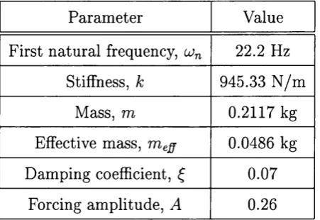
Before being able to use the numerical method described in section 2.4.2, in con junction with experimental data, calibration of the model must be made. This resolves to estim ating the values of the several param eters employed in the differ ential equations used in the model.
The experimental setup used in the work presented in later chapters, has been used in the past (Thompson et al. 1994; Bishop et al. 1996; Wagg et al. 1999). Some of the system parameters are therefore already known. The estimation of all used param eters is summarised below.
First n atu ral frequency, U n
The first natural frequency of the oscillator was determined experimentally. Fig ure 2.4 shows the power spectrum of an unforced non-impacting oscillation. The highest peak of the spectrum coincides with the first natural frequency of the beam, which is at a value of = 22.2 Hz.
Stiffness, k
The deflection, A at the free end of a cantilever beam acted upon by a static force
P at the free end (see figure 2.5) is given by: A = P L ^ / 3 E I , where L is the length of the beam, E is the Young’s modulus for the m aterial the beam is made of and / is the second moment of area of the beam ’s cross-section. The stiffness of the beam, k, is then given by: k = P / A = 3 E I/L ^ .
C H A P T E R 2. M O D E L LI N G SINGLE D E G R E E OF F R E E D O M V IB R O -IM PA G T S Y S T E M S 43
£
-2
- 6
22.2 44.4 66.6 88.8
Frequency (Hz)
F ig u r e 2.4: Power spectrum of an unforced non-im pacting oscillation.
F ig u r e 2.5: Deflection A, a t the free end of a cantilever beam , upon action of a