Volume 2009, Article ID 647262,21pages doi:10.1155/2009/647262
Research Article
Joint Motion Estimation and Layer Segmentation in
Transparent Image Sequences—Application to Noise Reduction
in X-Ray Image Sequences
Vincent Auvray,
1, 2Patrick Bouthemy,
1and Jean Li´enard
21INRIA Centre Rennes-Bretagne-Atlantique, Campus universitaire de Beaulieu, 35042 Rennes Cedex, France 2General Electric Healthcare, 283 rue de la Miniere, 78530 Buc, France
Correspondence should be addressed to Vincent Auvray,[email protected]
Received 27 November 2008; Accepted 6 April 2009
Recommended by Lisimachos P. Kondi
This paper is concerned with the estimation of the motions and the segmentation of the spatial supports of the different layers involved in transparent X-ray image sequences. Classical motion estimation methods fail on sequences involving transparent effects since they do not explicitly model this phenomenon. We propose a method that comprises three main steps: initial block-matching for two-layer transparent motion estimation, motion clustering with 3D Hough transform, and joint transparent layer segmentation and parametric motion estimation. It is validated on synthetic and real clinical X-ray image sequences. Secondly, we derive an original transparent motion compensation method compatible with any spatiotemporal filtering technique. A direct transparent motion compensation method is proposed. To overcome its limitations, a novel hybrid filter is introduced which locally selects which type of motion compensation is to be carried out for optimal denoising. Convincing experiments on synthetic and real clinical images are also reported.
Copyright © 2009 Vincent Auvray et al. This is an open access article distributed under the Creative Commons Attribution License, which permits unrestricted use, distribution, and reproduction in any medium, provided the original work is properly cited.
1. Introduction
Most image sequence processing and analysis tasks require an accurate computation of image motion. However, classical motion estimation methods fail in the case of image sequences involving transparent layers. Situations of trans-parency arise in videos for instance when an object is reflected in a surface, or when an object lies behind a translucent one. Transparency may also be involved in special effects in movies such as the representation of phantoms as transparent beings. Finally, let us mention progressive transition effects such asdissolve, often used in video editing. Some of these situations are illustrated onFigure 1.
In this paper, we are particularly concerned with the transparency phenomenon occuring in X-ray image sequences (even if the developed techniques can also be successfully applied to video sequences [1]). Since the radiation is successively attenuated by different organs, the resulting image is ruled by a multiplicative transparency
law (i.e., turned into an additive one by a log operator). ( The physics of the X-Ray resulting in additively transparent images are detailed inAppendix A.). For instance, the heart can be seen over the spine, the ribs and the lungs onFigure 2. When additive transparency is involved, the gray values of the different objects superimpose and the brightness constancy of points along their image trajectories, exploited for motion estimation [2], is no longer valid. Moreover, two different motion vectors may exist at the same spatial posi-tion. Therefore, motion estimation methods that explicitly tackle the transparency issue have to be developed.
(a)
(b)
(c)
Figure1: Examples of transparency configuration in videos. (a) Different reflections are shown, (b) three examples ofphantomeffects, and (c) one example of a dissolve effect for a gradual shot change.
motions, whereas a separation framework [3–5] leads to recover the gray value images of the different transparent objects. The latter can be handled so far in restricted situations only (e.g., specific motion must be assumed for at least one layer, the image globally includes only two layers), while we consider any type of motions and any number of layers. We aim at defining a general and robust method since we will apply it to noisy and low-contrasted X-ray image sequences.
We do not assume that the number of transparent layers in the image is known or limited. In contrast, we will determine it. We only assume a local two-layer configuration, that is, the image can be divided into regions where at most two transparent layers are simultaneously present. We will call such a situationbidistributed transparency. This is not a strong assumption since this is the most commonly encountered configuration in real image sequences.
Finally, we derive from the proposed transparent motion estimation method a general transparent motion compensa-tion method compatible with any spatio-temporal filtering technique. In particular, we propose a novel method for the temporal filtering of X-ray image sequences that avoids the appearance of severe artifacts (such as blurring), while taking advantage of the large temporal redundancy involved by the high acquisition frame rate.
The remainder of the paper is organized as follows. Section 2includes a state-of-the art on transparent motion estimation and introduces the fundamental transparent motion constraint. InSection 3, we present and discuss the different assumptions involved in the motion estimation problem statement.Section 4details the MRF-based frame-work that we propose, whileSection 5deals with the practical development of our joint transparent motion estimation and spatial layer segmentation method. In Section 6, we present the proposed filtering method, involving a novel transparent motion compensation procedure. We report in Section 7 experimental results for transparent motion
estimationon realistic test images as well as on numerous real clinical image sequences.Section 8presentsdenoisingresults on realistic test images and real clinical image sequences. Finally,Section 9contains concluding remarks and possible extensions.
2. Related Work on Transparent
Motion Estimation
are adopted, but the weak point is that transparency is not explicitly taken into account. The method [8] focuses on the problem of transparent motion estimation in angiograms to improve stenosis quantification accuracy. The motion fields are iteratively estimated by maximizing a phase correlation metric after removing the (estimated) contribution of the previously processed layer. However, it leads to interesting results only when one layer dominates the other one (which is not necessarily the case in interventional X-ray images).
Among the methods which explicitly tackle the trans-parency issue in the motion estimation process, we can dis-tinguish two main classes of approaches. The first one works in the frequency domain [9–11], but it must be assumed that the motions are constant over a large time interval (dozen of frames). These methods are therefore unapplicable to image sequences involving time-varying movements, such as cardiac motions in X-ray image sequences.
The second class of methods formulates the problem in the spatial image domain using the fundamental Transparent Motion Constraint (TMC) introduced by Shizawa and Mase [12], or its discrete version developed in [13]. The latter states that, if one considers the image sequenceIas the addition of two layersI1andI2(I =I1+I2), respectively, moving with velocity fieldsw1=(u1,v1) andw2=(u2,v2), the following
holds:
rx,y,w1,w2
=Ix+u1+u2,y+v1+v2,t−1
+Ix,y,t+ 1−Ix+u1,y+v1,t
−Ix+u2,y+v2,t=0,
(1)
where (x,y) are the coordinates of point p in the image. For sake of clarity, we do not make explicit thatw1 andw2
may depend on the image position. Expression (1) implicitly assumes that w1 and w2 are constant over time interval
[t−1,t+ 1]. Even if the hypothesis of constant velocity can be problematic at a few specific time instants of the heart cycle, (1) offers us with a reasonable and effective Transparent Motion Constraint (TMC) since the temporal velocity variations are usually smooth. This constraint can be extended ton layers by consideringn+ 1 images while extending the motion invariance assumption accordingly [13].
To compute the velocity fields using the TMC given by (1), a global functionJis usually minimized:
J(w1,w2)=
(x,y)∈I
rx,y,w1
x,y,w2
x,y2, (2)
wherer(x,y,w1(x,y),w2(x,y)) is given by (1) andIdenotes
the image grid.
Several methods have been proposed to minimize expres-sion (2), making different assumptions on the motions. The more flexible the hypothesis, the more accurate the estimation, but also the more complex the algorithm. A com-promise must be reached between measurement accuracy on one hand and robustness to noise, computational load and sensitivity to parameter tuning on the other hand.
Dense velocity fields are computed in [14] by adding a regularization term to (2), and in [15] by resorting to
a Markovian formalism. It enables to estimate nontrans-lational motions at the cost of higher sensitivity to noise and of high algorithm complexity. In contrast, stronger assumptions on the velocity fields are introduced in [16, 17] by considering thatw1 andw2 are constant on blocks
of the image, which allows fast but less accurate motion estimation. In [13], the velocity fields are decomposed on a B-spline basis, so that this method can account for complex motions, while remaining relatively tractable. However, the structure of the basis has to be carefully adapted to particular situations and the computational load becomes high if fine measurement accuracy is needed.
3. Transparent Motion Estimation
Problem Statement
We consider the general problem of motion estimation in
bidistributed transparency. It refers to transparent config-urations including any number of layers globally, but at most two locally. This new concept, which suffices to handle any transparent image sequence in practice, is discussed in Section 3.1.
To handle this problem, we resort to a joint segmentation and motion estimation framework. Because of transparency, we need to introduce a specific segmentation mechanism that allows distinct regions to superimpose, and to derive an original transparent joint segmentation and motion estimation framework.
Finally, to allow for a reasonably fast and robust method (able to handle X-Ray images), we consider transparen-cies involving parametric motion models as explained in Section 3.2.
3.1. Bi-Distributed Transparency. We do not impose any limitation on the number of transparent layers globally
involved in the image. Nevertheless, we assume that the images contain at most two layers at every spatial position
p, which is acceptable since three layers rarely superimpose in real transparent image sequences. We will refer to this configuration as thebidistributed transparency.
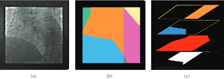
Even in the full transparency case encountered in X-ray exams, where acquired images result from cumulative absorption by X-ray tissues, the image can be nearly always divided into regions including at most two moving transparent layers, as illustrated onFigure 2. The only region involving three layers in this example is insignificant since the three corresponding organs are homogeneous in this area.
Unlike existing methods, we aim atexplicitlyextracting the segmentation of the image in its transparent layers, which is an interesting and exploitable output per se and is also required for the motion-estimation stage based on the two-layer TMC.
3.2. Transparent Motion Constraint with Parametric Models.
(a) (b) (c)
Figure2: (a) One image of X-ray exam yielding a situation of bidistributed transparency. (b) The segmentation of the image in its different regions: three two-layer regions (the orange region corresponds to the “heart and lungs”, the light blue one to “heart and diaphragm” and the pink one to “heart and spine”), two single-layer regions (the lungs in green and spine in yellow), and a small three-layer region (“heart and diaphragm and spine” in grey). (c) Its spatial segmentation into four transparent layers (i.e., their spatial supports, spine in orange, diaphragm in blue, heart in red and lungs in white). By definition, the spatial supports of the transparent layers overlap. The colors have been independently chosen in these two maps.
models offer a proper compromise since they can describe a large category of motions (translation, rotation, divergence, shear), while keeping the model simple enough to handle the transparency issue in a fast and tractable way. Our method could consider higher-order polynomial models as well, such as quadratic ones, if needed. Let us point out that in case of a more complex motion, the method is able to over-segment the corresponding layer in regions having a motion compatible with the considered type of parametric model. Complex transparent motions can still be accurately estimated at the cost of oversegmentation.
The velocity vector at point (x,y) for layer k is now defined bywθk(x,y)=(uθk(x,y),vθk(x,y)):
uθk
x,y=a1,k+a2,kx+a3,ky,
vθk
x,y=a4,k+a5,kx+a6,ky,
(3)
with θk = [a1,. . .,a6]T the parameter vector. We then
introduce a new version of the TMC (1) that we call the Parametric Transparent Motion Constraint (PTMC):
rx,y,wθ1,wθ2
=Ix+uθ1+uθ2,y+vθ1+vθ2,t−1
+Ix,y,t+ 1−Ix+uθ1,y+vθ1,t
−Ix+uθ2,y+vθ2,t
=0
(4)
withwθ1andwθ2given in (3).
The next section introduces the MRF-based framework that concludes the problem statement.
4. MRF-Based Framework
4.1. Observations and Remarks. We have to segment the image into regions including at most two layers to estimate the motion models associated to the layers from the PTMC (4). Conversely, the image segmentation will rely on the estimation of the different transparent motions. Therefore,
we have designed a joint segmentation and estimation frame-work based on a Markov Random Field (MRF) modeling. Ajointapproach is more reliable than a sequential one (as in [18]) since estimated motions can be improved using a proper segmentation and vice versa.
Joint motion estimation and segmentation frameworks have been developed for “classical” image sequences [19– 24], but have never been studied in the case of transparent images. In particular, we have to introduce a novel segmentation allowing regions to superimpose. Moreover, the bidistributed assumption implies to control the number of layers simultaneously present at a given spatial location.
The proposed method will result in an alternate minimization scheme between segmentation and estimation stages. To maintain a reasonable computational load, the segmentation is carried out at the level of blocks. Typically, the 1024 ×1024 images are divided in 32 × 32 blocks (for a total number of blocks S = 1024). We will see in Section 5.2that this block structure will also be exploited in the initialization step. According to the targeted application, the block size could be fixed smaller in a second phase of the algorithm. The pixel-level could even be progressively reached, if needed.
The blocks are taken as the sites s of the MRF model (Figure 3). We aim at labeling the blocks s according to the pair of transparent layers they are belonging to. Let e = {e(s),s = 1,. . .,S}denote the label field with e(s) = (e1(s),e2(s)), wheree1(s) ande2(s) designate the two layers present at sites.e1(s) ande2(s) are given the same value when the sitesinvolves one layer only. The spatial supports of the transparent layers can be straightforwardly inferred from the labeling of the two-layer regions (i.e., from the elements of each pair that forms the label).
Let us assume that the image comprises a total of K transparent layers, where K is to be determined. To each layer is attached an affine motion model of parametersθk(six
4.2. Global Energy Functional. We need to estimate the segmentation defined by the labels e(s), and the corre-sponding transparent motions defined by the parameters Θ. The estimates will minimize the following global energy functional:
F(e,Θ)=
s∈S
(x,y)∈s
ρC
rx,y,θe1(s),θe2(s)
−μη[s,e(s)]
+μ s,t
((1−δ(e1(s),e1(t)))(1−δ(e1(s),e2(t)))
+(1−δ(e2(s),e1(t)))(1−δ(e2(s),e2(t)))). (5)
The first term of (5) is the data-driven term based on the PTMC defined in (4). Instead of a quadratic constraint, we resort to a robust functionρC(·) in order to discard outliers,
that is, points where the PTMC is not valid [25]. We consider the Tukey function as robust estimator. It is defined by:
ρC(r)=
⎧ ⎪ ⎪ ⎪ ⎨ ⎪ ⎪ ⎪ ⎩
r6 6 −
C2r4 2 +
C4r2
2 if|r|< C, C6
6 otherwise.
(6)
It depends on a scale parameter C which defines the threshold above which the corresponding point will be considered as an outlier. To be able to handle any kind of images, we will determine C on-line as explained in Section 5.3.
The additional functionalη(·,·) is introduced in (5) to detect single layer configurations. It is a binary function which is 1 whensis likely to be a single layer site. It will be discussed inSection 4.3.
The last term of the global energy functional F(e,Θ) enforces the segmentation map to be reasonably smooth. We have to consider the four possible label transitions between two sites (involving two labels each).δ(·,·) is equal to 1 if the two considered elements are the same and equals 0 otherwise. Theμparameter weights the relative influence of the two terms. In other words, a penaltyμis added when introducing between two sites a region border involving a change in one layer only, and a penalty 2μwhen both layers are different. A transition between a mono-layer sites1and a bilayer sites2 will also imply a penaltyμ(as long as the layer present ins1 is also present ins2).μis determined in a content-adaptive way, as explained inSection 5.3.
4.3. Detection of a Single Layer Configuration. Over single layer regions, (1) is satisfied provided one of the two estimated velocities (for instancewθe1(s)) is close to the real
motion of this single layer whatever the value of the other velocity(wθe2(s)). The minimization of (5) without theη(·,·)
term would therefore not allow to detect single layer regions because a “imaginary” second layer would be introduced over these sites. Thus, we propose an original criterion to detect these areas.
We define the residual value:
νθe1(s),θe2(s),s
=
(x,y)∈s
rx,y,θe1(s),θe2(s) 2
. (7)
If it varies only slightly for different values ofθe2(s) (while keeping θe1(s) constant and equal to its estimate θe1(s)), it
is likely that the block s contains one single layer only, corresponding toe1(s).η(·,·) would be set to 1 in this case to favour the label (e1(s),e1(s)) over this site (and to 0 in the other cases).
Formally, to detect a single layer corresponding toθe1(s), we compute the mean value ν(θe1(s),s) of the residual ν(θe1(s),·,s) by applying n motions (defined by θj, j =
1,. . .,n,) to the second layer. We want to decide ifν(θe1(s),s)
is significantly different from the minimal residual on this block, ν(θe∗1(s),θe∗2(s),s), where (e
∗
1(s),e2∗(s)) are the current labels at sites. This minimal residual is in practice coming from the iterative minimization of (5) presented in Section 5.1.
To meet this decision independently of the image texture, we first compute a representative value for the residual of the image, given by
νmed=med
s∈S ν
θe∗
1(s),θe∗2(s),s
, (8)
and its median deviation
Δνmed=med
s∈S
νθe∗
1(s),θe2∗(s),s
−νmed. (9)
(This assumes that the motion models have been well estimated and the current labeling is correct on at least half the sites). Then, we set
η(s,e1(s),e2(s))=1 ifνθe∗1(s),s
−νθe∗1(s),θe∗2(s),s
< αΔνmed,
e1(s)=e2(s),
(10)
η(s,e1(s),e2(s))=0 otherwise, (11)
whereη(·,·) is the functional introduced in (5). This way, we favour the single layer label (e1(s),e1(s)) at siteswhen the condition (10) is satisfied. The same process is repeated to test forθe2(s)as the motion parameters of a (possible) single layer. In practice, we fixα=2.
5. Joint Parametric Motion Estimation and
Segmentation of Transparent Layers
(a) (b)
Figure3: MRF framework. (a) A processed image divided in blocks (36 blocks for the sake of clarity of the figure). (b) The graph associated with the introduced Markov model. The sites are plotted in blue and their neighbouring relations are drawn in orange.
(1)Initialization
(i) Transparent two-layer block-matching.
(ii) 3D Hough-transform applied to the computed pairs of displacements (simplified affine models). Each vote is assigned a confidence value related to the texture of the block and the reliability of the computed displacements. (iii) First determination of the global number of transparent layers and initialization of the affine motion models by
extraction of the relevant peaks of the accumulation matrix.
(iv) Layer segmentation initialization (using the maximum likelihood criterion).
Iteratively,
(2)Robust affine motion model estimation when the labels are fixed
Energy minimization using the IRLS technique. Multi-resolution incremental Gauss-Newton scheme. (3)Label field determination (segmentation) once the affine motion parameter are fixed
Energy minimization using the ICM technique (Iterative Conditional Modes). Criterion (10) is evaluated to detect single layer configurations in each blockS.
(4) Update of the number of layers (merge process). Finally,
(5) Introduction of a new layer if a given number of blocks verify relation (20). The overall algorithm is reiterated in this case.
Algorithm1: Joint transparent motion estimation and layer segmentation algorithm.
5.1. Minimization of the Energy Functional F. The energy functionalFdefined in (5) is minimized iteratively. When the motion parameters are fixed, we use the Iterative Conditional Mode (ICM) technique to update the labels of the blocks: the sites are visited randomly, and for each site the label that minimizes the energy functional (5) is selected.
Once the labels are fixed, we have to minimize the first term of (5), which involves a robust estimation. It can be solved using an Iteratively Reweighted Least Square (IRLS) technique which leads to minimize the equivalent functional [26]:
F1(Θ)=
s∈S
(x,y)∈s
αx,yrx,y,θe1(s),θe2(s) 2
, (12)
where α(x,y) denotes the weights. Their expression at the iteration jof the minimization is given by:
αjx,y=ρ
C
rx,y,θe1j−(s1),θ
j−1
e2(s)
2rx,y,θe1j−(1s),θ
j−1
e2(s)
(13)
withθ·j−1the estimate ofθ·computed at iteration j−1, and ρCthe derivative ofρC.
Even if each PTMC involves two models only, their addition over the entire image allows us to simultaneously estimate theK motion models globally present in the image by minimizing the functionalF1(Θ) of (12) (which is defined in a space of dimension 6K). If the velocity magnitudes were small, we could consider a linearized version of expression (12) (i.e., by relying on a linearized version of the expression r). Since large motions can occur in practice, we introduce a multiresolution incremental scheme exploiting Gaussian pyramids of the three consecutive images. At its coarsest levelL, motions are small enough to resort to a linearized version of functionalF1(Θ) (12). The minimization is then achieved using the conjugate gradient algorithm. Hence, first estimates of the motions parameters are provided, they are denotedθL
k,k=1,. . .,K.
At the level L−1, we initializeθL−1
i withθLi−1, where
aL−1
then writeθkL−1=θkL−1+ΔθLk−1, and we minimizeF1(Θ) with
respect to theΔθLk−1,k=1,. . . K, onceris linearized around
the θL−1
k , using the IRLS technique. This Gauss-Newton
method, iterated through the successive resolution levels until the finest one, allows us to simultaneously estimate the affine motion models of theKtransparent layers.
5.2. Initialization of the Overall Scheme. Such an alternate iterative minimization scheme converges if properly initial-ized. To initialize the motion estimation stage, we resort to a transparent block-matching technique that tests every possible pair of displacements in a given range [17]. More specifically, for each blocks, we compute
ζ(w1,w2,s)=
(x,y)∈s
rx,y,w1,w2 2
(14)
for a set of possible displacementsw1×w2, whereris given by (1). The pair of displacements (w1,w2) is the one which minimizes (14). This scheme is applied on a multiresolution representation of the images to reduce the computation time (it would be higher than in the case of nontransparent motions since the explored space is of dimension 4).
To extract the underlying layer motion models from the set of computed pairs of displacements, we apply the Hough transform on a three-dimension parameter space (i.e., a simplified affine motion model):
u=a1+a2x,
v=a4+a2y.
(15)
Indeed, restricting the Hough space to a 3D space obviously limits the computational complexity and improves the transform efficiency, while being sufficient to determine the number of layers and to initialize their motion models. Each displacementw=(u,v) votes for the parameters:
a1=a2x−u,
a4=a2y−v,
(16)
defining a straight line. The Hough space has to be dis-cretized in its three directions. Practically, we have chosen a one pixel step for the translational dimensionsa1 anda4, and for the divergence terma2a step corresponding to a one pixel displacement in the center of the image. An example of computed Hough accumulation matrix is given onFigure 4. If the layers include large homogeneous areas (which is the case in X-ray images), the initial block-matching is likely to produce a relatively large number of erroneous displacement estimates. To improve further the initialization stage, we adopt a continuous increment mechanism of the accumulation matrix based on a confidence value depending on the block texture.
To compute the confidence value associated to a block s and a displacement w1 (the other displacement being fixed to w2), we analyse the behavior of ζ(·,w2,s). If it remains close to its minimal value ζ(w1,w2,s), then the layer associated to w1 is homogeneous and w1 should be
−0.05
−0.04
−0.03
−0.02
−0.01 0 0.01 0.02 0.03 0.04 0.05
−8 −6
−4 −2 0 2 4 6 8
−5 0
5
Figure 4: Accumulation matrix in the space (a1,a4,a2), built
from the displacements computed by a transparent block-matching technique. These displacements are presented on the left ofFigure 5. The ground truth of the two motion models present in the image sequences are plotted in green and blue.
assigned a low confidence value. Conversely, ifζ(·,w2,s) has a clear minimum inw1, the corresponding layer is likely to be textured, andw1can be considered as reliable.
More precisely, we compute in each blocks:
c1(s)=
1n
Δw
ζ(w1+Δw,w2,s)−ζ(w1,w2,s) ,
c2(s)=
1n
Δw
ζ(w1,w2+Δw,s)−ζ(w1,w2,s) ,
(17)
where n is the number of tested displacements Δw. To normalize these coefficients, we compute their first quartilec over the image, and then assign to each blocksand computed displacementwi(i=1, 2) the valueci(s)/c(or 1 ifci(s)/c >
1). Then, the 25% more reliable computed displacements are assigned the value 1, whereas those that are less informative, or which are not correctly computed, are given a small confidence value.
The Hough transform allows us to cluster the reliable displacement vectors. We successively look for the dominant peaks in the accumulation matrix, and we decide that the corresponding motion models are relevant if they “originate” from at least five computed displacements that have not been considered so far. Conversely, a displacement computed by the transparent block-match technique is considered as “explained” by a given motion model if it is close enough to the mean velocity induced by this motion model over the considered block (in practice, distant by less than two pixels). This method yields a first evaluation of the number of layersK and an initialization of the affine motion models. Then, the label field is initialized by minimizing the first term of (5) only (i.e., we consider a maximum likelihood criterion).Figure 5illustrates the initialization stage.
(a) (b) (c)
Figure5: Example if the initialization stage for a symbolic example. (a) The displacements computed by the transparent block-matching. (b) The velocity fields corresponding to the affine models extracted by the Hough transform. Three layers are detected; they are plotted in red, green and blue. The erroneous displacements are plotted in black. (c) The true displacements.
parameterC of the robust functional, and the parameterμ weighting the relative influence of the data-driven and the smoothing term.Cis determined as follows:
r=med
p∈Ir
p,θe1(s),θe2(s)
,
Δr=1.48×med
p∈I
rp,θe1(s),θe2(s)
−r,
C=2.795×Δr
(18)
whenp is a pixel position, I refers to the image grid and whereθ· is the estimate ofθ·from the previous iteration of the minimization.
The use of the medians allows to evaluate representative valuesrandΔrof the “mean” and “deviation” residual values without being disturbed by the outliers. The factor 1.48 enables to unbiase the estimator ofΔr, and the factor 2.795 has been proposed by Tukey to correctly estimateC[27].
The μ parameter is determined in a content-adaptive way:
μ=λmed
s∈S
(x,y)∈s
ρC
rx,y,θe1(s),θe2(s)
. (19)
According to the targeted application,λcan be set to favour the data-driven velocity estimates (small λ), or to favour smooth segmentation (higherλ). In practice, the valueλ =
0.5 has proven to be a good tradeoffbetween regularization and oversegmentation.
5.4. Update of the Number of Transparent Layers. To update the numberK of transparent layers, we have designed two criteria. On one hand, two layers, the motion models of which are too close (typically, difference of one pixel on average over the corresponding velocity fields), are merged. Furthermore, a layer attributed to less than five blocks is discarded, and the corresponding blocks relabeled. On the other hand, we propose means to add a new layer if required, based on the maps of weights generated by the robust affine motion estimation stage.
The blocks where the current labels and/or the associated estimated motion models are not coherent with every pixel they contain should include low weight values delivered by the robust estimation stage for the outlier pixels. It then becomes necessary to add a new layer if a sufficient number of blocks containing a large number of pixels with low weights are detected. More formally, we use as indicator the number of weights smaller than a given threshold. The corresponding points will be referred to asoutliers. To learn which number of outliers per block is significant, we compute the median value of outliers N0 over the blocks, along with its median deviationΔNo. A blocksis considered
as mislabeled if its numberNo(s) of outliers verifies:
No(s)> No+γ·ΔNo (20)
withNo=med
s∈S No(s), (21)
ΔNo=med
s∈S |No(s)−No|. (22)
In practice, we set γ = 2.5. If more than five blocks are considered as mis-labeled, we add a new layer. We estimate its motion model by estimating an affine model from the displacement vectors supplied by the initial block-matching step in these blocks (using a least-square estimation), and we run the joint segmentation and estimation scheme on the whole image again.
6. Motion-Compensated Denoising Filter for
Transparent Image Sequences
In this section, we exploit the estimated transparent motions for a denoising application. To do so, we propose a way to compensate for the transparent motions, without having to
separatethe transparent layers.
6.1. Transparent Motion Compensation
layers and compensate the individual motion of each layer, layer per layer. However, the transparent layer separation problem has been solved in very restricted conditions only [5,8]. As a result, this cannot be applied in general situations as those encountered in medical image sequences.
Instead, we propose to globally compensate the trans-parent motions in the image sequence without prior layer separation. To do so, we propose to rearrange the PTMC (4) to form apredictionof the imageIat time t+ 1, based on the images at time instantst−1 andtand exploiting the two estimated affine motion modelsθ1andθ2:
Ip,t+ 1=Ip+wθ1
p,t+Ip+wθ2
p,t
−Ip+wθ1p+wθ2p,t−1
.
(23)
Equation (23) allows us to globally compensate for the transparent image motions. It enables to handle X-ray images that satisfy the bidistributed transparency hypothesis, that is, involving locally two layers, without limiting the total number of layersgloballypresent in the image.
Any denoising temporal filter can be made transparent-motion-compensated by considering, instead of past images, transparent-motion-compensated imagesIgiven by (23). As a consequence, details can be preserved in the images, and no blurring introduced if the transparent motions are correctly estimated.
However, relation (23) implies an increase of the noise level of the predicted image since three previous images are added. The variance of the noise corruptingIis the sum of the noise variances of the three considered images. This has adverse effects as demonstrated in the next subsection, if a simple temporal filter is considered.
6.1.2. Limitation. Transparent motion compensation can be added to any spatiotemporal filter. We will illustrate its limitation in the case of a pure temporal filter. More precisely, we consider the following temporal recursive filter [28]:
Ip,t+ 1=1−cp,t+ 1Ip,t+ 1
+cp,t+ 1Ip,t+ 1,
(24)
whereI(p,t+1) is the output of the filter, that is, the denoised image,I(p,t+ 1) is the predicted image andc(p,t+ 1) the filter weight. This simple temporal filter is frequently used since its implementation is straightforward and its behavior well-known. Spatial filtering tends to introduce correlated effects that are quite disturbing for the observer (especially when medical image sequences are played at high frame rates). This filter is usually applied in an adaptative way to account for incorrect prediction, which can be evaluated by the expression |I(p,t+ 1)−I(p,t+ 1)|. More specifically, the gain is defined as a decreasing function of the prediction error.
To illustrate the intrinsic limitation of such a transparent-motion compensated filter, we study its behavior under ideal conditions: the transparent motions are known as well as the
level of noise in the different images. Furthermore, we ignore the low-pass effect of interpolations. The noise variances σI2(t+ 1),σI2(t+ 1), andσ2(constant in time) of the images
I(t+ 1),I(t+ 1), andI(t), respectively, are related as follows (from (24)):
σ2
I(t+ 1)=(1−c(t+ 1))
2σ2+c(t+ 1)2σ2
I(t+ 1) (25)
under the assumption that the different noises are inde-pendent. On the other hand, (23) implies (for a recursive implementation of this filter):
σ2
I(t+ 1)=2σ
2
I(t) +σ
2
I(t−1). (26)
For an optimal noise filtering, one should choosec(t+ 1) so thatσ2(t+ 1) is minimized:
c(t+ 1)= 2σ
2
I(t) +σ
2
I(t−1)
2σI2(t) +σI2(t−1) +σ2. (27)
Equations (25) and (27) define a sequence (σI2(t))
t∈N. We
show inAppendix Cthat it asymptotically reaches a limit:
lim
t→ ∞σI(t)=
2
3σ 0.816σ. (28)
Even if we assume that the motions were known,transparent motion-compensated recursive temporal filter cannot allow for a significant denoising rate. Similarly, even if transparent motion-compensated spatiotemporal filters do not exhibit the exact same behavior, they denoise less efficiently that their noncompensated counterparts.
6.2. Hybrid Filter
6.2.1. Problem Statement. Transparent motion compensa-tion allows for a better contrast preservacompensa-tion since it avoids blurring. However, it affects the noise reduction efficiency by increasing the noise of the predicted image. We therefore propose to exploit the transparent motion compensation when appropriate only, to offer a better tradeoff between denoising power and information preservation. We distin-guish four local configurations:
(C0)Both layers are textured around pixelp. The global
transparent motion compensation is needed to pre-serve details. The filter output will rely onI(p,t+ 1) andI(p,t+ 1) only (instead ofI(p,t) andI(p,t+ 1) for the case without motion compensation).
(C1)The first layer only is texturedaround pixelp. We will
just perform the motion compensation of this layer but still applied to the compound intensity. The filter will then exploit I(p,t + 1),I(p + wθ1(p),t), and
here, but will be assigned a small weight because of its noise level):
Ip,t+ 1=αp,t+ 1Ip,t+ 1
+βp,t+ 1Ip+wθ1
p,t
+1−αp,t+ 1−βp,t+ 1Ip,t+ 1. (29)
Like in Section 6.1.2, explicit expressions can be computed for the optimal weights (see Table 1 for their expression in the case of a temporal hybrid filter).
(C2)The second layer only is texturedaround pixelp. We
use a combination ofI(p,t+ 1),I(p+wθ2(p),t), and
I(p,t+ 1).
(C3)Both layers are homogeneous around pixel p. The
four intensities can be used: I(p,t + 1),I(p +
wθ1(p),t),I(p+wθ2(p),t), andI(p,t+ 1).
A fifth configuration is added w.r.t. the motion estimation output.
(C4)The motion estimates are erroneous. In this case, we
duplicate I(p,t+ 1) only. This fifth configuration makes the hybrid filter adaptive, in the sense that it will keep displaying coherent images even if erroneous motion estimates are supplied.
6.2.2. Configuration Selection and Designed Hybrid Filtering.
This subsection deals with the detection of the local con-figuration among the five listed above. Let us assume that I1 only is textured around pixelp. Then, we can write (for convenience, we will writew1andw2instead ofwθ1(p) and
wθ2(p)):
Ip,t+ 1=I1
p,t+ 1+I2
p,t+ 1
=I1
p+w1,t+I2
p+w2,t
I1
p+w1,t+I2
p+w1,t
Ip+w1,t.
(30)
We have exploited in (30) the local lack of contrast of the layerI2. As a result, we can compareI(p,t+1) andI(p+w1,t) to decide whetherI2is uniform aroundp. To do so, we have to establish if these two values differ only because of the presence of noise, or if they actually correspond to different physical points. This is precisely the problem handled by adaptive filters.
We resort to the same mechanism. Rather than adopting a binary decision to select one given configuration Ci, that
would be visually disastrous since neighboring pixels would be processed differently,
(i) we first compute for each pixel p two factors: f1(p) associated to “the layer1is uniform” and f2(p) associated to “the layer2is uniform”. They are defined
as decreasing functions of|I(p,t+ 1)−I(p+w2,t)|
(resp.,|I(p,t+ 1)−I(p+w1,t)|). A third factor f12(p) is associated to “I(p,t+1)is a good prediction ofI(p,t+ 1)”. It is a decreasing function of|I(p,t+ 1)−I(p,t)|. This enables to associate each configuration (Ci),i=
0· · ·4, an appropriate weighting factor, as shown in (31).
(ii) we filter the image using relation (32) by considering in turn each configurationCi,i=0· · ·4, and we get
the output imagesI(Ci)(p,t).
(iii) we combine linearly these five output images as follows to yield the final denoised image:
Ip,t=f12
p1−f1
p1−f2
pI(C0)
p,t
+f12
p1−f1
pf2
pI(C1)
p,t
+f12
pf1
p1−f2
pI(C2)
p,t
+f12
pf1
pf2
pI(C3)
p,t
+1−f12
pI(C4)
p,t.
(31)
To summarize, the overall scheme comprises two modules:
(i) the first one filters the images based on different (transparent or nontransparent) motion compensa-tion schemes (Section 6.2.1).
(ii) the second module locally weights the five inter-mediate images according to the probability of the considered configuration (Section 6.2.2).
6.2.3. Temporal Hybrid Filter. In the case of a purely tempo-ral hybrid filter, the expression for a given configuration is defined by:
Ip,t+ 1=αp,tIp,t+ 1+βp,tIp+w1,t
+δp,tIp+w2,t+γp,tIp,t+ 1, (32)
whereα,β,δ, andγare filter weights locally specified.β=0 andδ=0 forC0;δ=0 forC1;β=0 forC2;β=0,δ =0
andγ =0 forC4. When the noise level of the input images
involved in (32) is known or estimated, one can analytically set the other weights for an optimal filtering (Table 1).
7. Transparent Motion Estimation Results
Table1: Optimal filter weights for the five possible configurations. The noise standard deviation noise of the acquired image is denotedσ, the one of the previous denoised imageσIand the one of the predicted imageσI.
Configuration α β
(C0)
σ2
I
σ2+σ2
I
0
(C1)
σ2 Iσ 2 I σ2 Iσ 2
I+σ2σ 2
I +σ 2
Iσ2
σ2σ2
I σ2 Iσ 2
I +σ2σ 2
I+σ 2
Iσ2
(C2)
σ2 Iσ 2 I σ2 Iσ 2
I+σ2σ 2
I +σ 2
Iσ2
0
(C3)
σ4 Iσ 2 I σ4 Iσ 2
I+σ2σ 2
Iσ 2
I +σ 2
Iσ2σ 2
I +σ 4
Iσ2
σ2σ2
Iσ 2 I σ4 Iσ 2
I +σ2σ 2
Iσ 2
I +σ 2
Iσ2σ 2
I+σ 4
Iσ2
(C4) 1 0
Configuration δ γ
(C0) 0
σ2
σ2+σ2
I
(C1) 0
σ2 Iσ 2 σ2 Iσ 2
I +σ2σ 2
I+σ 2
Iσ2
(C2)
σ2σ2
I σ2 Iσ 2
I+σ2σ 2
I +σ 2
Iσ2
σ2
Iσ2
σ2
Iσ 2
I +σ2σ 2
I+σ 2
Iσ2
(C3)
σ2
Iσ 2σ2
I σ4 Iσ 2
I+σ2σ 2
Iσ 2
I +σ 2
Iσ2σ 2
I +σ 4
Iσ2
σ4 Iσ 2 σ4 Iσ 2
I +σ2σ 2
Iσ 2
I +σ 2
Iσ2σ 2
I+σ 4
Iσ2
(C4) 0 0
all based on tests on the realistic generated image sequence (prepocessing, interpolation type, Block-Matching search range, accumulation matrix structure. . .). The method is therefore fully automatic.).
In this subsection, we focus on images containing two layers only, each one spread over the full image. It is indeed difficult to simultaneously assess the quality of the motion segmentation and of the layer segmentation (An erroneous segmentation that mislabels one block will dramatically impact the global estimation error (33), even if the considered block is low textured and little informative. The residual error would be a better error metric, yet it is much less intuitive.). The overall performance of the global method is discussed over real experiments inSection 7.2.
More specifically, we have applied our method on 250 three-frame sequences, the first layer (abdomen image) undergoing a translation and the second layer (heart image) an affine motion. To generate the affine motion of the second layer, we proceed in two steps. First, we randomly choose the two translational and the scaling (denotedh) parameters so that the resulting displacement magnitude lies in the range of −8 to 8 pixels. Then, we convert the obtained transformation into a set of affine motion models by allowing the two pairs of affine parametersa2,a6 on one hand, and a3,a5on the other hand, to vary from their reference value (resp., h and 0), in a range of respectively h±0.2h and
±0.2h. Consequently, the generated motions are similar to anatomic motions, while not perfectly following the model assumed by the Hough transform in the initialization step. The two generated motions are also required to sufficiently differ from each other, that is, from 2 pixels in average over the image grid (An observer would not perceive two distinct transparent layers otherwise!)
We have considered image sequences representative of diagnostic (high dose) and fluoroscopic (low dose) exams (with a noise of standard deviationσ=10 (SNR: 34 dB) and σ =20 (SNR: 28 dB) resp.), at different scatter rates (a real typical value being 20%). The images are coded on 12 bits, and their mean value is typically 500. Running the overall framework takes about 30 seconds for 288×288 images on a Pentium IV (2.4 GHz and 1 Go). The global estimation error is formally estimated below (33).
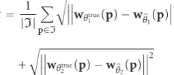
Table 2 contains the the mean value (in pixels) of the global estimation error computed from 250 tests, as well as its standard deviation and its median value:
=|I|1 p∈I
wθtrue
1 (p)−wθ1(p)
2
+wθtrue
2 (p)−wθ2(p)
2
(33)
wherewθtrue
i (resp.,wθi) refers to the velocity vectors (given
by the true (resp., estimated) models. We can observe that very satisfactory results are obtained. The average error raises to 0.36 pixels only for the most difficult diagnostic case. For comparison, the best method from the state of the art [8] reached a precision of about 2 pixels on similar data (involving quadratic motion models though). The estima-tion accuracy remains very good on the difficult fluoroscopic image sequences (σ = 20), where subpixel precision is maintained if the scatter rate is not too high. In this last case (50% scatter rate), the motion estimation remains interesting but is less accurate. The other indicators demonstrate the repeatability of the method over the different experiments.
Table 2: Performance evaluation of the proposed method for different noise levels and scatter rates: average, standard deviation and median value (in pixels) of the global error computed over 250 generated image sequences.
Metric on the global error Noise level Scatter rate
0% 20% 50%
Mean σ=10 0.22 0.27 0.36
σ=20 0.53 0.82 1.67
Standard deviation σ=10 0.63 0.66 0.70
Median
σ=20 0.78 0.93 1.65
σ=10 0.08 0.10 0.14
σ=20 0.25 0.41 1.00
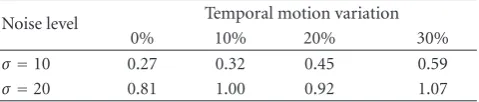
Table3: Average of the global estimation error for different noise levels and different temporal motion variations (with 20% scatter rate).
Noise level Temporal motion variation
0% 10% 20% 30%
σ=10 0.27 0.32 0.45 0.59
σ=20 0.81 1.00 0.92 1.07
intervals. This hypothesis may be critical for clinical image sequences at some time instants of the heart cycle. To test the violation of this assumption, we have carried out the following experiment.
We have randomly chosen two affine models (θ1 1,θ21) as explained above, and applied them between time instantst−
1 andt. We have then computed a second transparent motion field (θ2
1,θ22), allowing each coefficient to vary from 10, 20, or 30% around (θ1
1,θ21), and applied it between time instantst andt+ 1. This way, a sequence of three images with temporal motion variation is generated. We have evaluated the global errors between the estimated motion field and (θ1
1,θ21) on one hand, and (θ2
1,θ22) on the other hand. We report its mean value computed over 250 generated sequences inTable 3.
We can note aprogressivedegradation of the estimation accuracy with the amount of temporal motion change. Then, it is not that critical that the temporal motion constancy over two successive time intervals is not strictly verified. The transparent motion estimation for fluoroscopic images remains accurate, even if the two successive motions vary in a range of 30%.
7.2. Results on Real Clinical Image Sequences. The previous experiments are useful to study the behaviour of the pro-posed method, to fix the options and the parameters, and to quantitavely compare it to other motion estimation methods. However, it does not validate the relevance of the two-layer model per se, since the generated images themselves rely on this model. In this section, we present results obtained on real image sequences that demonstrate the bitransparency model validity.
We present motion estimation results out of three real clinical image sequences and one video. We display several
frames along with the estimated motion fields in Figures6– 8, at some interesting time instants of the sequences. The velocity fields are plotted with colored vectors, the length of which is twice the real displacement magnitude for sake of visibility.
The motion estimation quality is evaluated by visual inspection since no ground truth is available, and since the resulting displaced image differences are difficult to interpret due to the lack of contrast. Anyway, the reliability of the estimated motions is objectively demonstrated by the convincing results of transparent-motion-compensated denoising given inSection 8.
The image ofFigure 6corresponds to an area of about 5 cm×5 cm size, located between the heart (dark mass on the right) and the lungs (bright tissues). It also contains a static background where ribs are perceptible. In the considered region, the heart carries the lungs tissues along, so that they have the same apparent motion. The motions of the two layers are correctly estimated: the red arrow field corresponds to the static background (it is not plotted when it is exactly equal to 0), and the green one to the estimated affine model for the layer formed by the pair “heart and lungs”. Its motion is coherent with the observation, both during the diastole (first and third presented images) and the systole (second and last images).
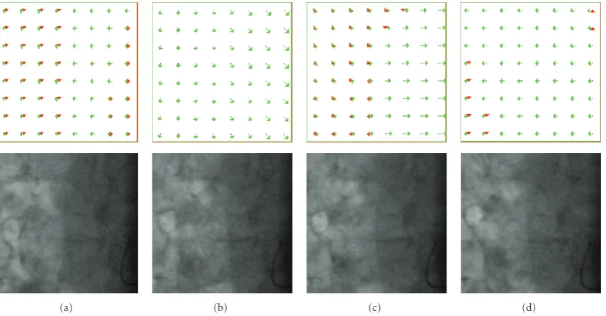
The sequence shown on Figures 7(a)–7(c) is a cardiac interventional image sequence. It globally involves three distinct transparent layers:
(i) the static background, which includes the contrasted surgical clips.
(ii) the set “diaphragm and lungs”. The diaphragm is the dark mass in the bottom left corner of the image, and the lungs form the bright tissues in the other half of the image. Their motions are close, so that they can be considered as forming a single moving layer. (iii) the heart is also visible, even if its layer is less textured:
it is the convex light-grey area on the right of the image. It can be easily seen on the first displayed image. A catheter (interventional tube) is inserted in one of its coronary, which has an visible motion different from the projected global motion of the heart (i.e., mainly inferred from the cardiac boundary perceptible in the image).
We first report results obtained at a time instant where the three layers are static (Figures7(a)–7(d)). Only one region is detected, which is correct: our method is still effective when no transparent motion is involved.
At a second time instant, the group “diaphragm and lungs” is still static. The velocity field supplied by the corresponding estimated motion model is plotted in red and the estimated motion of the heart in green (Figure 7(e)). Both motion models are correctly estimated. Interestingly, the movement of the catheter in the upper part of the image is properly segmented as well, even if it forms a thin structure in a noisy image sequence.
(a) (b) (c) (d)
Figure6: Four-estimated two-layer motion fields, along with the corresponding fluoroscopic image at four different time instants. One layer corresponds to the static background (ribs) and its estimated affine model is plotted in red. The other layer involves the heart and the lung tissues and its estimated affine model is plotted in green. (a), (c) instants are within in the diastole phase, (b), (d) ones in the systole phase.
appears to be undergoing independent visible motions. In this borderline situation (since we have three moving layers in some blocks), the method again proves to perform well: it manages to focus on the two dominant layers in the different regions. As a result, the red velocity field corresponds to the static background layer, the green one to the lungs layer, and the blue one to the heart motion layer.
The sequence presented on Figures8(a)–8(c)is a cardiac interventional image sequence. It depicts an about 5 cm× 5 cm area of the anatomy, where the heart (dark mass filling three quarters of the image, nearly static under the considered acquisition angulation) superimposes on the lungs (bright tissues in the upper right of the image). We give results for three distant instants of this sequence. The velocity fields plotted on Figures8(d)–8(f)are supplied by the affine motion models estimated at the three considered time instants.
A global two-layer transparency correctly explains the observed motions at the first time instant (Figure 8(d)). The green velocity vectors correspond to the group “lungs and diaphragm”, animated by the breathing, and the red field refers to the transparent layer of the heart (it is present all over the image but is not plotted when it is perfectly null). Let us also point out that the static background is merged with the heart layer.
It is necessary to introduce a bidistributed transparency configuration to explain the motions observed at the second considered time instant (Figure 8(e)). The red velocity field still refers to the (almost) static background, which now includes the mass of the heart and the diaphragm (motionless at this time). The blue velocity field corresponds
to the upward motion of breathing carrying along the lungs. The green velocity field accounts for a supplementary layer corresponding to the set of coronary arteries taken as a whole, the motion of which becomes perceptible. It is properly handled and correctly estimated. This demonstrates the ability of the method to focus on the two dominating motions even in situations of three-layer transparency (here, static layer, lungs layer and coronary arteries layer).
The last reported result (Figure 8(f)) highlights the performance of the method when situations of high com-plexity are encountered. All the different motions are indeed correctly estimated (by observing the sequence) even if oversegmentation is noticeable. Let us mention that a less fragmented spatial segmentation could be obtained by increasing the value of the regularization factorλ(19), but at the cost of a less accurate match between estimated motion models and observed motions. The trade-offhas to be met according to the targeted application.
Finally, Figure 9 reports experiments conducted on a sequence extracted from a movie, picturing a couple reflected on an apartment window. To our knowledge, it is the first time a real transparent video sequence is processed (we mean a sequence which has not been constructed for that purpose). The reflection superimposes to a panning view of the city behind. The camera is undergoing a smooth rotation, making the reflected faces and the city undergo two apparent translations with different velocities in the image. At some time instant, the real face of a character appears in the foreground but does not affect our method because of its robustness. The obtained segmentation and motion estimation are satisfying.
(a) (b) (c)
(d) (e) (f)
Figure7: Second example of a X-ray interventional cardiac image sequence, (a)–(c): Images acquired at three different time instants, (d), (e), (f): the corresponding velocity fields supplied by the estimated affine motion models, plotted in different colours according to the transparent layer they are belonging to. (a) Illustration of the method ability to detect single layer situations; (b) correct segmentation and estimation of the motions of small objects, even included in noisy images; (c) handling of a transparency situation with three simultaneous transparent layers in some areas (see main text).
(a) (b) (c)
(d) (e) (f)
Figure9: Example of a movie depicting two people reflected on an apartment window. From left to right and top to bottom: the first frame of the sequence; one of the three images corresponding to the reported results later in the sequence; the obtained segmentation into the transparent layer supports (the green polygonal line in the middle roughly encloses the reflected people); the velocity fields supplied by the estimated affine motion models; displaced frame differences computed by compensating the motion of one of the two layers.
8. Denoising Results
We have tested the proposed denoising method in the case of purely temporal filters because of their practical interest (explained inSection 6.1.2). Three denoising filters are compared: the adaptive recursive filter [28] without motion compensation (ANMCR) acting as a reference, the transparent-motion-compensated recursive filter (MCR) described inSection 6.1, and the proposed hybrid recursive filter (HR) developed inSection 6.2. The MCR and HR filters exploit transparent motions estimated by the method of Section 5.
The adaptive function of the ANMCR and MCR filters, taking into account the relation between filter gain and prediction error, is pictured on Figure 10. It has been designed heuristically to provide efficient noise reduction without introducing artifacts. It has three parts, defined by two thresholds (s1 =σ ands2 =2σ in practice): a constant part for the low prediction errors (where the coefficient is set to the optimal value for noise reductioncmax), a linear decreasing one in a transition area, and a vanishing one for large prediction errors. We have specified the three factors f1, f2, and f12of the hybrid filter in a similar way.cmaxis set to 1,s1to 1.5σands2to 2σfor that filter.
8.1. Results on Realistic Generated Image Sequences. We have tested the proposed denoising method on realistic synthetic image sequences simulating the X-ray imaging process and the transparency phenomenon (Appendix B.2). The obtained image sequence is corrupted by a strong noise typical of fluoroscopic exams (σ=20).
Table 4contains the evolution of the residual noise level of the filtered images. The transparent motion compensated filter soon reaches a denoising limit, as predicted by the theory. The hybrid filter performs slightly better than the ANMCR filter, as far as residual noise level is concerned.
cmax
s1
0 s2
Figure 10: Decreasing function used as adaptive function in the different filters. It has three parts: a constant one for small prediction errors, a linear one in a transition area, and a vanishing one for large prediction errors.
Table 4: Normalized residual noise evolution given by the rate
σ(t)/σ for a realistic synthetic image sequence typical of X-ray exams, processed by the adaptive temporal filter without motion compensation (ANMC), with transparent motion compensation (MC) and by the proposed hybrid filter (HR).
t 2 3 4 5 6 7 8
ANMCR 0.71 0.69 0.66 0.63 0.60 0.59 0.58
MCR 0.87 0.82 0.79 0.79 0.78 0.78 0.78
HR 0.76 0.66 0.60 0.57 0.56 0.55 0.54
The residual noise maps are given in Figure 11. They show that the hybrid filter preserves better the image details, and that the MCR filter also outperforms the ANMCR filter. However, the residual noise is much more perceptible in the case of MCR filter than for the other two filters.
Figure11: Residual noise of the eighth image of the generated sequence respectively obtained with the ANMCR filter, the MCR filter and the proposed HR filter (see main text).
(a) (b)
(c) (d)
Figure12: (a) Two time instants of a fluoroscopic sequence processed with the HR, (b) the ANMCR filter, (c), (d) one detail of each image is shown. (c) Highlights the better cardiac border contrast, and (d) the better lungs detail preservation.
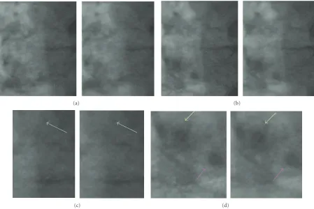
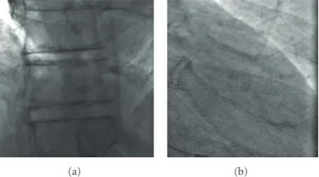
8.2. Results on Real Clinical Images. It is difficult to illustrate denoising results by means of static printed images, when the considered images are meant to be observed dynamically on a specific screen in a dark cath-lab. However, the major interest of our framework being its ability to improve the quality of real interventional images, we present three typical denoising results in this subsection.
Since the MCR performs noticeably worse than the two other filters, we will compare the performance of the ANMCR and HR filters only. The images processed with the former will be presented on the right of the figures, and those with the latter on the left, at different time instants. Both are heuristically parameterized to provide a visually equivalent global denoising effect, so that the difference of
performance will be mainly assessed based on the quality of contrast preservation and on the presence of artifacts. We have drawn arrows on the figures to highlight the regions of interest (that appear immediately on a dynamic display).
(a) (b)
Figure13: (a) Four-time instants of a fluoroscopic sequence processed with the HR, and (b) the ANMCR filter. We observe a better contrast preservation of the catheter with the hybrid filter.
(a) (b)
Figure14: (a) Fluoroscopic sequence processed with the HR, and (b) the ANMCR filter. The two images on the right correspond to a zoom on the region of interest of the two images of (a) .
with the HR filter (even if the printed figures do not give the immediate improvement impression that an observer has in ideal observation conditions). This is confirmed by the observation of the lungs.
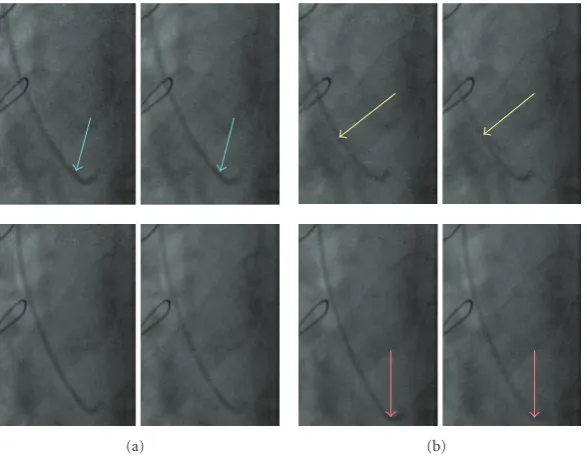
The second image sequence (Figure 13) corresponds to a cardiac exam where the catheter motion has been correctly handled by the transparent motion estimation module. We indeed observe that the catheter is more contrasted on the images processed by the HR filter than the ANMCR filter.
The last experiment exhibits the “noise tail” artifact induced by the ANMCR filter. When a moving textured object is detected by this filter, the corresponding area is kept without filtering in the output image. As a result, a region of the output image is more noisy than its neighborhood, which can be disturbing. In this situation, the hybrid filter is able to denoise the whole image, and thus does not introduce such artifacts. This phenomenon is pictured on Figure 14. We have added on the right of the figure a zoom on the region of interest. We observe that the curve corresponding to the moving border of the heart remains corrupted on the image
denoised with the ANMCR filter. This artifact disappears on the image processed by the HR filter.