Large, Pruned or Continuous Space Language Models on a GPU for Statistical Machine Translation

Large, Pruned or Continuous Space Language Models on a GPU

for Statistical Machine Translation

Holger Schwenk, Anthony Rousseau and Mohammed Attik

LIUM, University of Le Mans 72085 Le Mans cedex 9, FRANCE

[email protected]

Abstract

Language models play an important role in large vocabulary speech recognition and sta-tistical machine translation systems. The dominant approach since several decades are back-off language models. Some years ago, there was a clear tendency to build huge lan-guage models trained on hundreds of billions of words. Lately, this tendency has changed and recent works concentrate on data selec-tion. Continuous space methods are a very competitive approach, but they have a high computational complexity and are not yet in widespread use. This paper presents an ex-perimental comparison of all these approaches on a large statistical machine translation task. We also describe an open-source implemen-tation to train and use continuous space lan-guage models (CSLM) for such large tasks. We describe an efficient implementation of the CSLM using graphical processing units from Nvidia. By these means, we are able to train an CSLM on more than 500 million words in 20 hours. This CSLM provides an improve-ment of up to 1.8 BLEU points with respect to the best back-off language model that we were able to build.

1 Introduction

Language models are used to estimate the proba-bility of a sequence of words. They are an impor-tant module in many areas of natural language pro-cessing, in particular large vocabulary speech recog-nition (LVCSR) and statistical machine translation (SMT). The goal of LVCSR is to convert a speech signalxinto a sequence of wordsw. This is usually

approached with the following fundamental equa-tion:

w∗ = arg max

w P(w|x)

= arg max

w P(x|w)P(w) (1)

In SMT, we are faced with a sequence of wordse in the source language and we are looking for its best translation f into the target language. Again, we apply Bayes rule to introduce a language model:

f∗ = arg max

f P(f|e)

= arg max

f P(e|f)P(f) (2)

Although we use a language model to evaluate the probability of the produced sequence of words, w andf respectively, we argue that the task of the lan-guage model is not exactly the same for both ap-plications. In LVCSR, the LM must choose among a large number of possible segmentations of the phoneme sequence into words, given the pronuncia-tion lexicon. It is also the only component that helps to select among homonyms, i.e. words that are pro-nounced in the same way, but that are written dif-ferently and which have usually different meanings (e.g.ate/eightorbuild/billed). In SMT, on the other hand, the LM has the responsibility to chose the best translation of a source word given the context. More importantly, the LM is a key component which has to sort out good and bad word reorderings. This is known to be a very difficult issue when translat-ing from or into languages like Chinese, Japanese or German. In LVCSR, the word order is given by the time-synchronous processing of the speech signal. Finally, the LM helps to deal with gender, number,

etc accordance of morphologically rich languages, when used in an LVCSR as well as an SMT system. Overall, one can say that the semantic level seems to be more important for language modeling in SMT than LVCSR. In both applications, so called back-off n-gram language models are the de facto standard since several decades. They were first introduced in the eighties, followed by intensive research on smoothing methods. An extensive comparison can be found in (Chen and Goodman, 1999). Modified-Kneser Ney smoothing seems to be the best perform-ing method and it is this approach that is almost ex-clusively used today.

Some years ago, there was a clear tendency in SMT to use huge LMs trained on hundreds on bil-lions (101_{1) of words (Brants et al., 2007). The}

au-thors report continuous improvement of the trans-lation quality with increasing size of the LM train-ing data, but these models require a large cluster to train and to perform inference using distributed stor-age. Therefore, several approaches were proposed to limit the storage size of large LMs, for instance (Federico and Cettolo, 2007; Talbot and Osborne, 2007; Heafield, 2011).

1.1 Continuous space language models

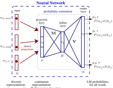
The main drawback of back-off n-gram language models is the fact that the probabilities are estimated in a discrete space. This prevents any kind of inter-polation in order to estimate the LM probability of an n-gram which was not observed in the training data. In order to attack this problem, it was pro-posed to project the words into a continuous space and to perform the estimation task in this space. The projection as well as the estimation can be jointly performed by a multi-layer neural network (Bengio and Ducharme, 2001; Bengio et al., 2003). The ba-sic architecture of this approach is shown in figure 1. A standard fully-connected multi-layer per-ceptron is used. The inputs to the neural network are the indices of the n−1 pre-vious words in the vocabulary hj=wj−n+1,

. . . , wj−2, wj−1 and the outputs are the posterior

probabilities ofallwords of the vocabulary:

P(wj =i|hj) ∀i∈[1, N] (3) where N is the size of the vocabulary. The input uses the so-called 1-of-n coding, i.e., theith word of

projection

layer hidden layer

output layer input

projectionsshared

continuous representation: representation: indices in wordlist

LM probabilities discrete

for all words probability estimation

Neural Network

N

wj−1 P

H

N

P(wj=1|hj)

wj−n+1

wj−n+2

P(wj=i|hj)

P(wj=N|hj)

Pdimensional vectors

ck

oi M

V dj

p1=

pN=

pi=

Figure 1: Architecture of the continuous space LM.hj

denotes the contextwj−n+1, . . . , wj−1. P is the size of

one projection andH,Nis the size of the hidden and out-put layer respectively. When short-lists are used the size of the output layer is much smaller then the size of the vocabulary.

the vocabulary is coded by setting theith element of the vector to 1 and all the other elements to 0. The ith line of theN×P dimensional projection matrix corresponds to the continuous representation of the ith word. Let us denotecl these projections,dj the hidden layer activities,oi the outputs,pi their soft-max normalization, andmjl,bj,vij andki the hid-den and output layer weights and the corresponding biases. Using these notations, the neural network performs the following operations:

dj = tanh X

l

mjlcl+bj !

(4)

oi = X

j

vijdj+ki (5)

pi = eoi / N X

r=1

eor ₍₆₎

The value of the output neuronpiis used as the prob-ability P(wj =i|hj). Training is performed with the standard back-propagation algorithm minimiz-ing the followminimiz-ing error function:

E =

N X

i=1

tilog pi+β 

 X

jl

m2_jl+X

ij

v_ij2



 (7)

proba-bility should be 1.0 for the next word in the training sentence and 0.0 for all the other ones. The first part of this equation is the cross-entropy between the out-put and the target probability distributions, and the second part is a regularization term that aims to pre-vent the neural network from overfitting the training data (weight decay). The parameterβ has to be de-termined experimentally.

The CSLM has a much higher complexity than a back-off LM, in particular because of the high di-mension of the output layer. Therefore, it was pro-posed to limit the size of the output layer to the most frequent words, the other ones being predicted by a standard back-off LM (Schwenk, 2004). All the words are still considered at the input layer.

It is important to note that the CSLM is still an n-gram approach, but the notion of backing-off to shorter contexts does not exist any more. The model can provide probability estimates for any possible n-gram. It also has the advantage that the complex-ity only slightly increases for longer context win-dows, while it is generally considered to be unfea-sible to train back-off LMs on billions of words for orders larger than 5.

The CSLM was very successfully applied to large vocabulary speech recognition. It is usually used to rescore lattices and improvements of the word er-ror rate of about one point were consistently ob-served for many languages and domains, for in-stance (Schwenk and Gauvain, 2002; Schwenk, 2007; Park et al., 2010; Liu et al., 2011; Lamel et al., 2011). More recently, the CSLM was also suc-cessfully applied to statistical machine translation (Schwenk et al., 2006; Schwenk and Est`eve, 2008; Schwenk, 2010; Le et al., 2010)

During the last years, several extensions were pro-posed in the literature, for instance:

• Mikolov and his colleagues are working on the use of recurrent neural networks instead of multi-layer feed-forward architecture (Mikolov et al., 2010; Mikolov et al., 2011).

• A simplified calculation of the short-list prob-ability mass and the addition of an adaptation layer (Park et al., 2010; Liu et al., 2011)

• the so-called SOUL architecture which allows to cover all the words at the output layer instead

of using a short-list (Le et al., 2011a; Le et al., 2011b), based on work by (Morin and Bengio, 2005; Mnih and Hinton, 2008).

• alternative sampling in large corpora (Xu et al., 2011)

Despite significant and consistent gains in LVCSR and SMT, CSLMs are not yet in widespread use. Possible reasons for this could be the large com-putational complexity which requires flexible and carefully tuned software so that the models can be build and used in an efficient manner.

In this paper we provide a detailed comparison of the current most promising language modeling tech-niques for SMT: huge back-off LMs that integrate all available data, LMs trained on data selected with respect to its relevance to the task by a recently pro-posed method (Moore and Lewis, 2010), and a new very efficient implementation of the CSLM which integrates data selection.

2 Continuous space LM toolkit

2.1 Parallel processing

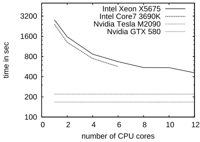
The computational power of general purpose pro-cessors like those build by Intel or AMD has con-stantly increased during the last decades and opti-mized libraries are available to take advantage of the multi-core capabilities of modern CPUs. Our CSLM toolkit fully supports parallel processing based on Intel’s MKL library.1 Figure 2 shows the time used to train a large neural network on 1M examples. We trained a 7-gram CSLM with a projection layer of size 320, two hidden layers of size 1024 and 512 re-spectively, and an output layer of dimension 16384 (short-list). We compared two hardware architec-tures:

• a top-end PC with one Intel Core i7 3930K pro-cessor (3.2 GHz, 6 cores).

• a typical server with two Intel Xeon X5675 pro-cessors (2×3.06 GHz, 6 cores each).

We did not expect a linear increase of the speed with the number of threads run in parallel, but nev-ertheless, there is a clear benefit of using multiple cores: processing is about 6 times faster when run-ning on 12 cores instead of a single one. The Core i7 3930K processor is actually slightly faster than the Xeon X5675, but we are limited to 6 cores since it can not interact with a second processor.

2.2 Running on a GPU

In parallel to the development efforts for fast general purpose CPUs, dedicated hardware has been devel-oped in order to satisfy the computational needs of realistic 3D graphics in high resolutions, so called graphical processing units (GPU). Recently, it was realized that this computational power can be in fact used for scientific computing, e.g. in chem-istry, molecular physics, earth quake simulations, weather forecasts, etc. A key factor was the avail-ability of libraries and toolkits to simplify the pro-gramming of GPU cards, for instance the CUDA toolkit of Nvidia.2 The machine learning commu-nity has started to use GPU computing and several toolkits are available to train generic networks. We have also added support for Nvidia GPU cards to the

1

http://software.intel.com/en-us/articles/intel-mkl

2_{http://developer.nvidia.com/cuda-downloads}

100 200 400 800 1600 3200

0 2 4 6 8 10 12

time in sec

number of CPU cores Intel Xeon X5675 Intel Core7 3690K Nvidia Tesla M2090 Nvidia GTX 580

Figure 2: Time to train on 1M examples on various hard-ware architectures (the speed is shown in log scale).

CSLM toolkit. Timing experiments were performed with two types of GPU cards:

• a Nvidia GTX 580 GPU card with 3 GB of memory. It has 512 cores running at 1.54 GHz.

• a Nvidia Tesla M2090 card with 6 GB of mem-ory. It has 512 cores running at 1.3 GHz.

As can be seen from figure 2, for these network sizes the GTX 580 is about 3 times faster than two Intel X5675 processors (12 cores). This speed-up is smaller than the ones observed in other studies to run machine learning tasks on a GPU, probably be-cause of the large number of parameters which re-quire many accesses to the GPU memory. For syn-thetic benchmarks, all the code and data often fits into the fast shared memory of the GPU card. We are continuing our work to improve the speed of our toolkit on GPU cards. The Tesla M2090 is a little bit slower than the GTX 580 due to the lower core fre-quency. However, it has a much better support for double precision floating point calculations which could be quite useful when training large neural net-works.

3 Experimental Results

AFP APW NYT XIN LTW WPB CNA old avrg recent old avrg recent old avrg recent old avrg recent all all all

Using all the data:

Words 151M 547M 371M 385M 547M 444M 786M 543M 364M 105M 147M 144M 313M 20M 39M

Perplex 167.7 141.0 138.6 192.7 170.3 163.4 234.1 203.5 197.1 162.9 126.4 121.8 170.3 269.3 266.5

After data selection:

Words 36M 77M 96M 62M 77M 89M 110M 54M 44M 23M 35M 38M 69M 6M 7M 23% 26% 26% 16% 14% 20% 14% 10% 12% 22% 24% 26% 22% 30% 18% Perplex 160.9 135.0 131.6 185.3 153.2 151.1 201.2 173.6 169.5 159.6 123.4 117.7 153.1 263.9 253.2

Table 1: Perplexities on the development data (news wire genre) of the individual sub-corpora in the LDC Gigaword corpus, before and after data selection by the method of (Moore and Lewis, 2010).

as 15th feature function and the coefficients of all the feature functions are optimized by MERT. The CSLM toolkit includes scripts to perform this task.

3.1 Baseline systems

The Arabic/English SMT system was trained on par-allel and monolingual data similar to those avail-able in the well known NIST OpenMT evaluations. About 151M words of bitexts are available from LDC out of which we selected 41M words to build the translation model. The English side of all the bitexts was used to train the target language model.

In addition, we used the LDC Gigaword corpus version 5 (LDC2011T07). It contains about 4.9 bil-lion words coming from various news sources (AFP and XIN news agencies, New York Times, etc) for the period 1994 until 2010. All corpus sizes are given after tokenization.

For development and tuning, we used the OpenMT 2009 data set which contains 1313 sen-tences. The corresponding data from 2008 was used as internal test set. We report separate results for the news wire part (586 sentence, 24k words) and the web part (727 sentences, 24k words) since we want to compare the performance of the various LMs for formal and more informal language. Four reference translations were available. Case and punctuation were preserved for scoring.

It is well known that it is better to build LMs on the individual sources and to interpolate them, in-stead of building one LM on all the concatenated data. The interpolation coefficients are tuned by op-timizing the perplexity on the development corpus using an EM procedure. We split the huge

Giga-word corpora AFP, APW, NYT and XIN into three parts according to the time period (old, average and recent). This gives in total 15 sub-corpora. The sizes and the perplexities are given in Table 1. The inter-polated 4-gram LM of these 15 corpora has a per-plexity of 87 on the news part.

If we add the English side of all the bitexts, the perplexity can be lowered to 71.1. All the observed n-grams were preserved, e.g. the cut-off forn-gram counts was set to 1 for all orders. This gives us an huge LM with 1.4 billion 4-grams, 548M 3-grams and 83M bigrams which requires more 26 GBytes to be stored on disk. This LM is loaded into mem-ory by the Moses decoder. This takes more than 10 minutes and requires about 70 GB of memory.

Moses supports memory mapped LMs, like IRSTLM or KENLM, but this was not explored in this study. We call this LM “big LM”. We believe that it could be considered as a very strong base-line for a back-off LM. We did not attempt to build higher order back-off LM given the size require-ments. For comparison, we also build a small LM which was trained on the English part of the bitexts and the recent XIN corpus only. It has a perplexity of 78.9 and occupies 2 GB on disk (see table 2).

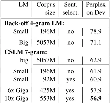
3.2 Data selection

We have reimplemented the method of Moore and Lewis (2010) to select the most appropriate LM data based on the difference between the sentence-wise entropy of an in-domain and out-of domain LM.

170 180 190 200 210 220 230 240

0 10 20 30 40 50 60 70 80 90 100

Perplexity

Percentage of corpus AFP

APW NYT XIN

Figure 3: Decrease in perplexity when selecting data with the method proposed in (Moore and Lewis, 2010).

data is used, reaching a minimum using about 20% of the data only. The improvement in the perplexity can reach 20% relative. Figure3 shows the perplex-ity for some corpora in function of the size of the selected data. Detailed statistics for all corpora are given in Table 1 for the news genre.

Unfortunately, these improvements in perplexity almost vanish when we interpolate the individual language models: the perplexity is 86.6 instead of 87.0 when all the data from the Gigaword corpus is used. This LM achieves the same BLEU score on the development data, and there is a small improve-ment of 0.24 BLEU on the test set (Table 2). Never-theless, the last LM has the advantage of being much smaller: 7.2 instead of 25 GBytes. We have also per-formed the data selection on the concatenated texts of 4.9 billion words. In this case, we do observe an decrease of the perplexity with respect to a model trained on all the concatenated data, but overall, the perplexity is higher than with an interpolated LM (as expected).

Px BLEU

LM Dev Size Dev Test

Small 78.9 2.0 GB 56.89 49.66

Big 71.1 26 GB 58.66 50.75

Giga 87.0 25.0 GB 57.08 50.08

GigaSel 86.6 7.2 GB 57.03 50.32

Table 2: Comparison of several 4-gram back-off lan-guage models. See text for explanation of the models.

3.3 Continuous space language models

The CSLM was trained on all the available data using the resampling algorithm described in (Schwenk, 2007). At each epoch we randomly re-sampled about 15M examples. We build only one CSLM resampling simultaneously in all the corpora. The short list was set to 16k – this covers about 92% of then-gram requests. Since it is very easy to use large context windows with an CSLM, we trained right away 7-grams. We provide a comparison of different context lengths later in this section. The networks were trained for 20 epochs. This can be done in about 64 hours on a server with two Intel X5675 processors and in 20 hours on a GPU card.

This CSLM achieves a perplexity of 62.9, to be compared to 71.1 for the big back-off LM. This is a relative improvement of more than 11%, but actually we can do better. If we train the CSLM on thesmall corpusonly, i.e. the English side of the bitexts and the recent part of the XIN corpus, we achieve a per-plexity of 61.9 (see table 3). This clearly indicates that it is better to focus the CSLM on relevant data.

Random resampling is a possibility to train a neu-ral network on very large corpora, but it does not guarantee that all the examples are used. Even if we resampled different examples at each epoch, we would process at most 300M different examples (20 epochs times 15M examples). There is no reason to believe that we randomly select examples which are appropriate to the task (note, however, that the re-sampling coefficients are different for the individual

LM Corpus Sent. Perplex

size select. on Dev

Back-off 4-gram LM:

Small 196M no 78.9

Big 5057M no 71.1

CSLM 7-gram:

big 5057M no 62.9

Small 196M no 61.9

Small 92M yes 60.9

6x Giga 425M yes. 57.9

10x Giga 553M yes. 56.9

Small LM Huge LM CSLM

Genre 4-gram back-off 7-gram

News 49.66 50.75 52.28

Web / 35.17 36.53

Table 4: BLEU scores on the test set for the translation from Arabic into English for various language models.

corpora similar to the coefficients of an interpolated back-off LM). Therefore, we propose to use the data selection method of Moore and Lewis (2010) to con-centrate the training of the CSLM on the most in-formative examples. Instead of sampling randomly n-grams in all the corpora, we do this in the selected data by the method of (Moore and Lewis, 2010). By these means, it is more likely that we train the CSLM on relevant data. Note that this has no impact on the training speed since the amount of resampled data is not changed.

The results for this method are summarized in Ta-ble 3. In a first experiment, we used the selected part of the recent XIN corpus only. This reduces the per-plexity to 60.9. In addition, if we use the six or ten most important Gigaword corpora, we achieve a per-plexity of 57.9 and 56.9 respectively. This is 10% better than resampling blindly in all the data (62.9

→ 56.9). Overall, the 7-gram CSLM improves the perplexity by 20% relative with respect to the huge 4-gram back-off LM (71.1→56.9).

Finally, we used our best CSLM to rescore the n-best lists of the Arabic/English SMT system. The baseline BLEU score on the test set, news genre, is 49.66 with the small LM. This increases to 50.75 with the big LM. It was actually necessary to open the beam of the Moses decoder in order to observe such an improvement. The large beam had no effect when the small LM was used. This is a very strong baseline to improve upon. Nevertheless, this result is further improved by the CSLM to 52.28, i.e. a significant gain of 1.8 BLEU. We observe similar behavior for the WEB genre.

All our networks have two hidden layers since we have observed that this slightly improves perfor-mance with respect to the standard architecture with only one hidden layer. This is a first step towards so-called deep neural networks (Bengio, 2007), but we have not yet explored this systematically.

Order: 4-gram 5-gram 6-gram 7-gram

Px Dev: 63.9 59.5 57.6 56.9

BLEU Dev: 59.76 60.11 60.29 60.26

BLEU Test: 51.91 51.85 52.23 52.28

Table 5: Perplexity on the development data (news genre) and BLEU scores of the continuous space language mod-els in function of the context size.

In an 1000-best list for 586 sentences, we have a total of 14M requests for 7-grams out of which more than 13.5M were processed by the CSLM, e.g. the short list hit rate is almost 95%. This resulted in only 2670 forward passes through the network. At each pass, we collected in average 5350 probabilities at the output layer. The processing takes only a couple of minutes on a server with two Xeon X5675 CPUs. One can of course argue that it is not correct to compare 4-gram and 7-gram language models. However, building 5-gram or higher order back-off LMs on 5 billion words is computationally very ex-pensive, in particular with respect to memory usage. For comparison, we also trained lower order CSLM models. It can be clearly seen from Table 5 that the CSLM can take advantage of longer contexts, but it already achieves a significant improvement in the BLEU score at the same LM order (BLEU on the test data: 50.75→51.91).

The CSLM is very space efficient: a saved net-work occupies about 600M on disk in function of the network architecture, in particular in function of the size of the continuous projection. Loading takes only a couple of seconds. During training, 1 GByte of main memory is sufficient. The memory require-ment duringn-best rescoring essentially depends on the back-off LM that is eventually charged to deal with out-off short-list words. Figure 4 shows some example translations.

4 Conclusion

This paper presented a comparison of several pop-ular techniques to build language models for sta-tistical machine translation systems: huge back-off models trained on billions of words, data selection of most relevant examples and a highly efficient im-plementation of continuous space methods.

!"#ا%&تا()&ث(+أ-./01234ي67ا8497:;ي<=>7اث%.27ا!=?:@A0&:@2Aا-/<B7ا9C<Aا<4ز%7ا(EBF:1C ث(+G;دو9Aاوم:K7ا849.7ةد%M7ا!>Nا<&-?OPK2Aاء:RSA:;-T:S1S@7ا01)Aا(EBFوي<=>7اث%.27ا .!U4(=7ا!S#%7%R@27اة9"#Vا

Back-off LM:The minister inspected the sub-committee integrated combat marine pollution with oil, which includes the latest equipment lose face marine pollution and chemical plant in the port specializing in monitoring the quality of the crude oil supplier and with the most modern technological devices.

CSLM: The minister inspected the integrated sub-committee to combat marine pollution

with oil, which includes the latest equipment deal with marine pollution and inspect the chemical plant in the port specializing in monitoring the quality of the crude oil supplier, with the most modern technological devices.

Google: The minister also inspected the sub-center for integrated control of marine pollution with oil, which includes the latest equipment on the face of marine pollution and chemical plant loses port specialist in quality control of crude oil and supplied

يو%R7اW&:X<>7اء:"XY:"F:&ا927اما<2+:;()FZX:S[X%S;

Back-off LM:Pyongyang is to respect its commitments to end nuclear program.

CSLM: Pyongyang promised to respect its commitments to end the nuclear program.

Google: Pyongyang is to respect its obligations to end nuclear program.

. \S]:Aا\&:)7ال_`ر<@2&0@3;د_>7اb?ف:d2`Yات:S.1);ن:>7:f%=.g&م:N

Back-off LM: The Taliban militants in kidnappings in the country over the past two years.

CSLM: Taliban militants have carried out kidnappings in the country repeatedly during

the past two years.

Google:The Taliban kidnappings in the country frequently over the past two years.

Figure 4: Example translations when using the huge back-off and the continuous space LM. For comparison we also provide the output of Google Translate.

case, 26 GB on disk and 70 GB of main memory for a model trained on 5 billions words. The data selec-tion method proposed in (Moore and Lewis, 2010) is very effective at the corpus level, but the observed gains almost vanish after interpolation. However, the storage requirement can be divided by four.

The main contributions of this paper are sev-eral improvements of the continuous space language model. We have shown that data selection is very useful to improve the resampling of training data in large corpora. Our best model achieves a per-plexity reduction of 20% relative with respect to the best back-off LM we were able to build. This gives an improvement of up to 1.8 BLEU points in a

very competitive Arabic/English statistical machine translation system.

We have also presented a very efficient imple-mentation of the CSLM. The tool can take advan-tage of modern multi-core or multi-processor com-puters. We also support graphical extension cards like the Nvidia 3D graphic cards. By these means, we are able to train a CSLM on 500M words in about 20 hours. This tool is freely available.3 By these means we hope to make large-scale continu-ous space language modeling available to a larger community.

Acknowledgments

This work has been partially funded by the French Government under the project COSMAT

(ANR-09-CORD-004) and the European Commission under the project FP7 EuromatrixPlus.

References

Yoshua Bengio and Rejean Ducharme. 2001. A neu-ral probabilistic language model. InNIPS, volume 13, pages 932–938.

Yoshua Bengio, Rejean Ducharme, Pascal Vincent, and Christian Jauvin. 2003. A neural probabilistic lan-guage model.JMLR, 3(2):1137–1155.

Yoshua Bengio. 2007. learning deep architectures for AI. Technical report, University of Montr´eal.

Thorsten Brants, Ashok C. Popat, Peng Xu, Franz J. Och, and Jeffrey Dean. 2007. Large language models in machine translation. InEMNLP, pages 858–867. Stanley F. Chen and Joshua T. Goodman. 1999. An

empirical study of smoothing techniques for language modeling. Computer Speech & Language, 13(4):359– 394.

Marcello Federico and Maura Cettolo. 2007. Efficient handling of n-gram language models for statistical ma-chine translation. InSecond Workshop on SMT, pages 88–95.

Kenneth Heafield. 2011. KenLM: Faster and smaller language model queries. InSixth Workshop on SMT, pages 187–197.

Philipp Koehn, Hieu Hoang, Alexandra Birch, Chris Callison-Burch, Marcello Federico, Nicola Bertoldi, Brooke Cowan, Wade Shen, Christine Moran, Richard Zens, Chris Dyer, Ondrej Bojar, Alexandra Con-stantin, and Evan Herbst. 2007. Moses: Open source toolkit for statistical machine translation. In ACL, demonstration session.

L. Lamel, J.-L. Gauvain, V.-B. Le, I. Oparin, , and S. Meng. 2011. Improved models for mandarin speech-to-text transcription. InICASSP, pages 4660– 4663.

H.S. Le, A. Allauzen, G. Wisniewski, and F. Yvon. 2010. Training continuous space language models: Some practical issues. InEMNLP, pages 778–788.

H.S. Le, I. Oparin, A. Allauzen, J-L. Gauvain, and F. Yvon. 2011a. Structured output layer neural net-work language model. InICASSP, pages 5524–5527. H.S. Le, I. Oparin, A. Messaoudi, A. Allauzen, J-L.

Gau-vain, and F. Yvon. 2011b. Large vocabulary SOUL neural network language models. InInterspeech.

X. Liu, M. J. F. Gales, and P. C. Woodland. 2011. Im-proving LVCSR system combination using neural net-work language model cross adaptation. InInterspeech, pages 2857–2860.

Tom´aˇs Mikolov, Martin Karafi´at, Luk´aˇs Burget, Jan ˇ

Cernock´y, and Sanjeev Khudanpur. 2010. Recurrent neural network based language model. InInterspeech, pages 1045–1048.

T. Mikolov, S. Kombrink, L. Burget, J.H. Cernocky, and S. Khudanpur. 2011. Extensions of recurrent neural network language model. In ICASSP, pages 5528– 5531.

Andriy Mnih and Geoffrey Hinton. 2008. A scalable hierarchical distributed language model. InNIPS. Robert C. Moore and William Lewis. 2010. Intelligent

selection of language model training data. In ACL, pages 220–224.

Frederic Morin and Yoshua Bengio. 2005. Hierarchi-cal probabilistic neural network language model. In

Proceedings of the Tenth International Workshop on Artificial Intelligence and Statistics.

Junho Park, Xunying Liu, Mark J. F. Gales, and Phil C. Woodland. 2010. Improved neural network based lan-guage modelling and adaptation. InInterspeech, pages 1041–1044.

Holger Schwenk and Yannick Est`eve. 2008. Data selec-tion and smoothing in an open-source system for the 2008 NIST machine translation evaluation. In Inter-speech, pages 2727–2730.

Holger Schwenk and Jean-Luc Gauvain. 2002. Connec-tionist language modeling for large vocabulary contin-uous speech recognition. In ICASSP, pages I: 765– 768.

Holger Schwenk, Daniel D´echelotte, and Jean-Luc Gau-vain. 2006. Continuous space language models for statistical machine translation. InProceedings of the COLING/ACL 2006 Main Conference Poster Sessions, pages 723–730.

Holger Schwenk. 2004. Efficient training of large neu-ral networks for language modeling. InIJCNN, pages 3059–3062.

Holger Schwenk. 2007. Continuous space language models. Computer Speech and Language, 21:492– 518.

Holger Schwenk. 2010. Continuous space language models for statistical machine translation.The Prague Bulletin of Mathematical Linguistics, (93):137–146. David Talbot and Miles Osborne. 2007. Smoothed

bloom filter language models: Tera-scale lms on the cheap. InEMNLP, pages 468–476.