R E S E A R C H
Open Access
An efficient implementation of iterative
adaptive approach for source localization
Gang Li
1*, Hao Zhang
1, Xiqin Wang
1and Xiang-Gen Xia
2Abstract
The iterative adaptive approach (IAA) can achieve accurate source localization with single snapshot, and therefore it has attracted significant interest in various applications. In the original IAA, the optimal filter is performed for every scanning angle grid in each iteration, which may cause the slow convergence and disturb the spatial estimates on the impinging angles of sources. In this article, we propose an efficient implementation of IAA (EIAA) by modifying the use of the optimal filtering, i.e., in each iteration of EIAA, the optimal filter is only utilized to estimate the spatial components likely corresponding to the impinging angles of sources, and other spatial components corresponding to the noise are updated by the simple correlation of the basis matrix with the residue. Simulation results show that, in comparison with IAA, EIAA has significant higher computational efficiency and comparable accuracy of source angle and power estimation.
Keywords: sparse recovery; iterative adaptive approach; source localization.
1 Introduction
Source localization is a fundamental problem in a wide range of applications including communications, radar, and acoustics, and many algorithms have been presented in the literature during recent decades. The Fourier-based algorithms suffer from the low resolution and the high sidelobes. Some methods based on subspace processing, e.g., Capon beamforming [], MUSIC [], ESPRIT [], and other subspace-based algorithms [, ], provide super-resolution for uncorrelated sources with sufficient num-ber of snapshots. However, in the case of few snapshots, the performances of these subspace-based methods will degrade sharply.
Recently, the source localization problem has been con-verted into a sparse recovery framework, because the number of actual sources of interest is generally much smaller than the number of potential source locations in the region to be observed. A kind of algorithms of sparse recovery is based on iterative weighted least squares, e.g., the FOCal Underdetermined System Solver (FOCUSS)
*Correspondence: [email protected]
1Tsinghua National Laboratory for Information Science and Technology
(TNList), Department of Electronic Engineering, Tsinghua University, Beijing 100084, China
Full list of author information is available at the end of the article
[], the Sparse Learning via Iterative Minimization (SLIM) [], the iterative adaptive approach (IAA) [], etc. Here, we are interested in IAA, which is able to provide accu-rate source localization with single snapshot and has at-tracted significant interest in various applications [–]. IAA is non-parametric and it achieves accurate estimates of angles and powers of the sources by iterative opera-tions []. The spatial component on every potential angle is estimated by optimal filtering, which passes the signal from the current angle without distortion and fully sup-presses the interferences from other angles. The iteration is terminated when the norm of the difference between two successive spatial estimates is smaller than a certain threshold. However, it is time consuming to perform opti-mal filtering on all potential angles, since in general we are only interested in several angles where the actual sources are located. Moreover, the excessive estimation of the spa-tial components on the angles that are outside the actual source position set may result in a slow convergence. In this article, we propose an efficient implementation of IAA (EIAA) by modifying the use of the optimal filtering, i.e., in each iteration, the optimal filter is only utilized to estimate the spatial components likely corresponding to the actual signal sources, and other spatial components correspond-ing to the noise are updated by the simple correlation of the basis matrix with the residue. It will be shown that
EIAA has significant faster convergence speed and com-parable accuracy of source angle and power estimation. In [, ], two fast implementations of IAA have been pro-posed by using the matrix computation technique such as Gohberg-Semencul decomposition, etc. It is noted that the way of the computational burden reduction in this article is different from [, ]: herein, we focus on reducing the number of running optimal filtering procedures, while [, ] focus on improving the computational efficiency of the optimal filtering procedure. In addition, similar to the al-gorithms mentioned above, we are only interested in the unambiguous angle solution, which depends on the ratio of interelement spacing of the array to the wavelength. In the case that the angle ambiguity occurs, we refer to [– ] for resolving the ambiguity.
The remainder of this article is organized as follows. The signal model and the original IAA are introduced in Sec-tion . The EIAA algorithm is proposed in SecSec-tion . The proposed EIAA is evaluated by some simulations in Sec-tion . Concluding remarks are presented in SecSec-tion .
2 Signal model and IAA
Suppose that K potential far-field narrowband signals are impinging on an M-element array from directions
{θ,θ, . . . ,θK}. In single snapshot case, the output mea-surement vector of the array can be expressed as
y=As+e,
whereAis theM×Kbasis matrix and is defined byA= [a(θ),a(θ), . . . ,a(θK)],sis theK× vector denoting the complex amplitudes of the sources,eis the additive noise. Considering anM-element linear array as shown in Fig-ure , thekth column ofAcorresponding to the potential source directionθkcan be represented by
a(θk) =
e–jπxcos(θk)/λ,e–jπxcos(θk)/λ,
. . . ,e–jπxMcos(θk)/λT,
where{x,x, . . . ,xM}are the positions of theMelements of the array, respectively,λis the wavelength, (·)Tdenotes transpose. In sparse recovery framework, the potential
Figure 1 The geometry of sensors and sources.
source numberK is rather considered to be the number of discretized angle grids. Assume thatsis sparse, i.e., the number of actual sources is much smaller thanK. Consider the line-spectrum model and let P=diag{p,p, . . . ,pK}, whosekth diagonal elementpkcontains the power atkth scanning angle grid. The problem of interest is recovering the spatial components {p,p, . . . ,pK}, and the positions and the amplitudes of the peaks of{p,p, . . . ,pK}directly provide the locations and the powers of the sources. IAA [] achieves this goal as summarized in Table , where the superscript (i) denotes theith iteration.
3 Efficient implementation of IAA
It is noted that step (b) in Table gives an optimal filter in terms ofθk, which reserves the signal from angleθk with-out distortion and fully suppresses the interferences (sig-nals from other angles). In each iteration the optimal filter-ing is performedKtimes for all angles{θ,θ, . . . ,θK}. This is computationally extravagant, because in general we are only interested in the angle set where the actual sources are located. Moreover, for the indexkcorresponding toθk outside the angle set of actual sources,pkmost likely de-pends on the noise power, and the iterative estimation of
pk may increase the actual number of iterations required for the convergence. Based on the above observations, we modify IAA as described in Table .
The main difference between the proposed EIAA and the original IAA lies in the estimation of spatial com-ponents that are outside the actual source location set. As seen from step (b) in Table ,{θkwith indexk∈(i)} are considered to be likely angle candidates where actual
Table 1 IAA algorithm.
Initialization:pˆ(0)k = |aH(θk)y|2
[aH(θk)a(θk)]2fork= 1, 2,. . .,K. Repeat:
(a) Calculate the correlation matrix byRˆ(i)=APˆ(i)AH.
(b) Estimate the spatial components bypˆ(ki)=| aH(θk)·(Rˆ(i))–1·y
aH(θk)·(Rˆ(i))–1·a(θk)|
2, fork= 1, 2,. . .,K.
(c) If the norm of the difference betweenPˆ(i–1)andPˆ(i)is smaller than a threshold, i.e.,δ(i)=K k=1[pˆ
(i–1)
k –pˆ
(i)
k]2<ε, the iteration is stopped; otherwise
Table 2 EIAA algorithm.
Initialization: letpˆ(0)k = |aH(θk)y|2
[aH(θk)a(θk)]2
fork= 1, 2,. . .,K; let the residuer(0)=y;
Repeat:
(a) Calculate the correlation matrix byRˆ(i)=APˆ(i)AH;
Let the index support set(i)=∅and the principal spatial component set (i)=∅.
(b)Whilethe relative residue is larger than a threshold, i.e.,r
(i)2 2
y2 2
>ξ
Find the indexnlcorresponding to the largest entry in the vector [pˆ(1i),pˆ (i) 2,. . .,pˆ
(i)
K];
Expand the index support set by(i)={(i),n
l};
Expand the principal spatial component set by (i)={ (i),| a
H(θ nl)·(Rˆ(i))–1·y aH(θnl)·(Rˆ(i))–1·a(θnl)|
2};
Calculate the residue byr(i)=y– (AH
(i)A(i))
–1AH
(i)y, where the matrixA(i)consists of the columns ofAwith indicesk∈
(i);
Update the spatial estimate bypˆ(ki)= |aH(θk)r(i)|2
[aH(θk)a(θk)]2, fork= 1, 2,. . .,K. end While
(c) Restore the principal spatial components bypˆ(ki)= (i)(k), fork∈(i).
(d) If the norm of the difference betweenPˆ(i–1)andPˆ(i)is smaller than a threshold, i.e.,δ(i)=K k=1[pˆ
(i–1)
k –pˆ
(i)
k]2<ε, the iteration is stopped; otherwise
leti=i+ 1 and go to a).
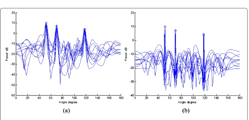
Figure 2 Spatial estimation results by 10 Monte-Carlo trials. (a)IAA estimates,(b)EIAA estimates.
Table 3 Performances of IAA and EIAA for various SNR.
SNR 0 dB 5 dB 10 dB 15 dB 20 dB
erangleEIAA–erangleIAA –0.297◦ –0.114◦ –0.107◦ –0.015◦ –0.004◦ erpowerEIAA –erpowerIAA –0.087 –0.393 –0.543 –0.489 –0.373
RTR of EIAA and IAA 0.131 0.118 0.081 0.072 0.070
sources are located. Then, the spatial components corre-sponding to the actual source locations are updated by op-timal filtering, and other spatial components correspond-ing to the noise are updated by simple correlation of the columns of basis matrix with the residue. This implies that the excessive estimation of noise components is avoided. Compared with the original IAA, EIAA can significantly
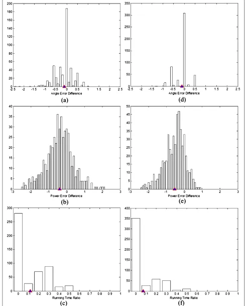
Any-Figure 3 Performance comparison of IAA and EIAA. (a-c)ForSNR= 5 dB;(d-f)forSNR= 10 dB.(a, d)Angle error differenceerangleEIAA–erangleIAA;
(b, e)power error differenceerpowerEIAA–er power
way, the number of the selected principle components, i.e., the required times of optimal filtering procedure, is usu-ally much smaller thanK, which is guaranteed by the prior assumption of sparse signal property. () The relaxation of the estimation of spatial components corresponding to noise leads to stable and fast convergence.
4 Simulations
In this section, some examples are provided to evaluate the performance of the proposed EIAA in single snapshot case. Consider a uniform linear array ofM= sensors with the interelement spacingλ/. The additional noise is assumed Gaussian with zero mean and variance σ, and the SNR is defined as log(Ln=pn/(Lσ)). The angle scanning grid is uniform in the range from ◦to ◦with ◦increment between adjacent angle candidates.
Assume that there are three sources at ◦, ◦, and ◦ withp= dB,p= dB, andp= dB powers,
respec-tively. For SNR = dB, Figure shows the spatial esti-mates of IAA and EIAA. The true source locations are in-dicated by circles, and the results of ten Monte-Carlo trials are plotted. One can see that both of IAA and EIAA can ac-curately indicate the locations and powers of the sources, while EIAA shows sharper peaks.
The performances of IAA and EIAA are compared via histograms over trials in Figure , where SNR = dB for (a-c) and SNR = dB for (d-f ). The thresholds in Ta-ble are set by ε= . and ξ = .. The source
lo-calization error is defined by erangle =
i=(θˆi–θi)/ and the power estimation error is defined by erpower =
i=(pˆi–pi)/. Figure a,b,d,e represent histograms of erangleEIAA– erangleIAA and erpowerEIAA – erpowerIAA , and the triangles in-dicate the centroids of the histograms. It is obvious that most values of erangleEIAA– erangleIAA and erpowerEIAA– erpowerIAA are close to zero, which implies that EIAA is comparable with IAA in terms of the accuracy of angle and power estimation. Moreover, the negative centroids indicate that the estima-tion accuracy of EIAA is slightly better than that of IAA. Figure c,f represent the histograms of the running time ratio (RTR) of EIAA and IAA, and the triangles indicate the histogram centroids, and it can be seen EIAA is certainly faster than IAA since all results of RTR are smaller than one. Moreover, the centroids of RTR about . indicate that the computational efficiency is significantly improved by the proposed EIAA. For various SNR, the performances of IAA and EIAA are compared in Table , where each re-sult is obtained by finding the centroid position of the his-togram over trials (see triangle position in Figure for example). One can see that EIAA has slightly better angle and power estimation accuracy than IAA. As for the com-putational efficiency, the running time of EIAA is less than % of that of IAA for various SNR.
5 Conclusion
In this article, EIAA algorithm is proposed for source lo-calization. By selecting the principal components of spatial estimate in each iteration, the optimal filter is only utilized to estimate the spatial components likely corresponding to the actual signal sources, and the other spatial compo-nents corresponding to noise are updated by the simple correlation of the basis matrix with the residue. Compared with the original IAA that performs optimal filtering on every scanning angle grid in each iteration, EIAA shows higher computational efficiency and slightly better accu-racy of angle and power estimation.
Acknowledgements
This study was supported in part by the National Natural Science Foundation of China under Grant 40901157, and in part by the National Basic Research Program of China (973 Program) under Grant 2010CB731901, in part by the Doctoral Fund of Ministry of Education of China under Grant 200800031050, and in part by Tsinghua National Laboratory for Information Science and Technology (TNList) Cross-discipline Foundation. Xia’s work was supported by the National Science Foundation (NSF) under Grant CCF-0964500 and the World Class Univerrsity (WCU) Program, National Research Foundation, Korea.
Competing interests
The authors declare that they have no competing interests.
Authors’ contributions
GL carried out the algorithm design and the drafted the manuscript. HZ and XW participated in convergence analysis. X-GX participated in statistical analysis. All authors read and approved the final manuscript.
Author details
1Tsinghua National Laboratory for Information Science and Technology
(TNList), Department of Electronic Engineering, Tsinghua University, Beijing 100084, China.2Department of Electrical and Computer Engineering,
University of Delaware, Newark, DE 19716, USA.
Received: 11 July 2011 Accepted: 12 January 2012 Published: 12 January 2012
References
1. J Capon, High resolution frequency-wavenumber spectrum analysis. Proc IEEE57(8), 1408–1418 (1969)
2. RO Schmidt, Multiple emitter location and signal parameter estimation. IEEE Trans Antennas Propag3, 276–280 (1986)
3. R Roy, T Kailath, ESPRIT - estimation of signal parameters via rotational invariance techniques. IEEE Trans Acoust Speech Signal Process37(7), 984–995 (1989)
4. S Bourennane, C Fossati, J Marot, About noneigenvector source localization methods. EURASIP J Adv Signal Process2008(2008). Article ID 480835
5. Q Wang, Q Jiang, Simulation of matched field processing localization based on empirical mode decomposition and Karhunen-Loeve expansion in underwater waveguide environment. EURASIP J Adv Signal Process
2010(2010). Article ID 483524
6. IF Gorodnitsky, BD Rao, Sparse signal reconstruction from limited data using FOCUSS: a re-weighted minimum norm algorithm. IEEE Trans Signal Process45(3), 600–616 (1997)
7. X Tan, W Roberts, J Li, P Stoica, Sparse learning via iterative minimization with application to MIMO radar imaging. IEEE Trans Signal Process59(3), 1088–1101 (2011)
8. T Yardibi, J Li, P Stoica, M Xue, AB Baggeroer, Source localization and sensing: a nonparametric iterative adaptive approach based on weighted least squares. IEEE Trans Aerosp Electron Syst46(1), 425–443 (2010) 9. W Roberts, P Stoica, J Li, T Yardibi, FA Sadjadi, Iterative adaptive approaches
10. P Stoica, J Li, J Ling, Missing data recovery via a nonparametric iterative adaptive approach. IEEE Signal Process Lett16(4), 241–244 (2009) 11. NR Butt, A Jakobsson, Coherence spectrum estimation from nonuniformly
sampled sequences. IEEE Signal Process Lett17(4), 339–342 (2010) 12. M Xue, L Xu, J Li, IAA spectral estimation: fast implementation using the
Gohberg-Semencul factorization. IEEE Trans Signal Process59(7), 3251–3261 (2011)
13. GO Glentis, A Jakobssony, Efficient implementation of iterative adaptive approach spectral estimation techniques. IEEE Trans Signal Process59(9), 4154–4167 (2011)
14. J Sun, J Tian, G Wang, S Mao, Doppler ambiguity resolution for multiple PRF radar using iterative adaptive approach. Electron Lett46(23), 1562–1563 (2010)
15. G Li, J Xu, Y-N Peng, X-G Xia, An efficient implementation of a robust phase unwrapping algorithm. IEEE Signal Process Lett14(6), 393–396 (2007) 16. W Wang, X-G Xia, A closed-form Robust Chinese Remainder Theorem and
its performance analysis. IEEE Trans Signal Process58(11), 5655–5666 (2010)
doi:10.1186/1687-6180-2012-7