R E S E A R C H
Open Access
Matched steering vector searching based
direction-of-arrival estimation using
acoustic vector sensor array
Yu Ao
*, Ling Wang, Jianwei Wan and Ke Xu
Abstract
The acoustic vector sensor (AVS) array is a powerful tool for underwater target’s direction-of-arrival (DOA) estimation without any bearing ambiguities. However, traditional DOA estimation algorithms generally suffer from low signal-to-noise ratio (SNR) as well as snapshot deficiency. By exploiting the properties of the minimum variance distortionless response (MVDR) beamformer, a new DOA estimation method basing on matched steering vector searching is proposed in this article. Firstly, attain the rough estimate of the desired DOA using the traditional algorithms. Secondly, set a small angular interval around the crudely estimated DOA. Thirdly, make the view direction vary in the view interval, and for each view direction, calculate the beam amplitude response of the MVDR beamformer, and find the minimum of the amplitude response. Finally, the pseudo-spatial spectrum is achieved, and the accurate estimate of the desired DOA can be obtained through peak searching. Computer simulations verify that the proposed method is efficient in DOA estimation, especially in low SNR and insufficient snapshot data scenarios.
Keywords:Acoustic vector sensor (AVS) array, Direction-of-arrival (DOA) estimation, Minimum variance distortionless response (MVDR), Pseudo-spatial spectrum, Steering vector
1 Introduction
An acoustic vector sensor (AVS) consists of an omnidir-ectional acoustic pressure receiver and a dipole-like directional particle velocity receiver [1]. AVS measures the three Cartesian components of the particle velocity as well as the scalar acoustic pressure at a single point in sound field synchronously and independently [2]. Com-pared with the standard acoustic pressure sensors, the intrinsic directivity gives an AVS two advantages. One is that the directly measured directional information permits the arrays made up of acoustic vector sensors to improve the accuracy of target detection and source localization without increasing array aperture. The other is that the left/right ambiguity problem, from which an acoustic pressure sensor array always suffers, never arise. Even a single AVS is capable of localizing a source in the whole space [3], which is of great practical significance.
Due to the considerable performance and the huge po-tential demands in underwater applications, AVS has
developed rapidly in theory and been widely used in many engineering fields during the last two decades, especially in passive DOA estimation. Since Nehorai and Paldi first introduce the AVS array measurement model to the signal processing research community [4], diverse types of DOA estimation algorithms have been proposed [5–13]. Hawkes and Nehorai adapt the MVDR (also known as Capon) approach to AVS array [5]. Wong and Zoltowski link the subspace-based methods, which in-clude the estimation of signal parameters via rotational invariance technique (ESPRIT) [6], root multiple signal classification (MUSIC) [7], and self-initiating MUSIC [8] to the AVS array. The wideband source localization and wideband beamforming issues are discussed in [9, 10] respectively. A 2-D DOA estimation algorithm using the propagator method (PM) is proposed in [11]. Liu et al. introduce a 2-D DOA estimation method for coherence sources with a sparse AVS array [12]. Han and Nehorai put forward a new class of nested vector-sensor arrays which is capable of significantly increasing the degrees of freedom [13]. In [14], a modified particle filtering algorithm for DOA Tracking basing on a single AVS is
© The Author(s). 2019Open AccessThis article is distributed under the terms of the Creative Commons Attribution 4.0 International License (http://creativecommons.org/licenses/by/4.0/), which permits unrestricted use, distribution, and reproduction in any medium, provided you give appropriate credit to the original author(s) and the source, provide a link to the Creative Commons license, and indicate if changes were made.
* Correspondence:[email protected]
proposed. With the help of an L-shaped sparsely-distrib-uted vector sensor array, Si et al. present a novel 2-D DOA and polarization estimation method to handle the scenario where uncorrelated and coherent sources coexist [15]. Recently, several novel techniques such as the parallel profiles with linear dependencies (PARALIND) model [16], compressed sensing [17], and partial angular sparse repre-sentation method [18] have been investigated for DOA estimation using the AVS array.
In the practical ocean environment, the signal-to-noise ratio (SNR) is usually quite low and the snapshot data is usually insufficient. These disadvantages may lead to ser-ious performance degradation for DOA estimation when the traditional techniques are applied. To overcome these problems, a number of new algorithms have appeared in the literature [19,20–26]. Ichige et al. put forward a modi-fied MUSIC algorithm by using both the amplitude and phase information of noise subspace [19]. A new method for DOA estimation is proposed in [20] through iteratively subspace decomposition. In [21], by means of signal covariance matrix reconstruction, the noise subspace is precisely estimated and the DOA estimation performance is improved. With the help of the optimization method, [22] presented a noise subspace-based iterative algorithm for direction finding. Recently, a few new techniques were combined with DOA estimation, such as the sparse recov-ery algorithm [23], the sparse decomposition technique [24], the compressive sensing theory [25], and the multiple invariance ESPRIT [26].
In this paper, we investigate the feature of the Capon approach in depth. The design principle of the MVDR beamformer can be described as minimizing the variance of interference and noise at the output of the beamfor-mer, while ensuring the distortionless response of the beamformer towards a selected view direction, which is naturally hoped to equal the direction of the desired source. However, in the case that the view direction does not point to the desired source precisely, even a very slight mismatch will lead the phenomenon known as signal cancellation [27], i.e., the beamformer will misin-terpret the desired signal as an interference and put a null in the direction of the desired signal. Generally speaking, signal cancellation has an unfavorable effect on beamforming and DOA estimation, and several stud-ies have been carried out on suppressing such effects [28–30]. However, in this paper, we find that the signal cancellation phenomenon can be utilized to attain a better performance of DOA estimation by searching the matched steering vector. What is more, differing from all of the methods mentioned in [19, 20–26], our study is based on the AVS array; hence, the bearing ambiguity is removed.
The rest part of this paper is structured as follows. In Section 2, we state the mathematical model for the
measurements of an AVS array. In Section 3, we propose our DOA estimation algorithm, give its steps, and analyze the relation between the presented algorithm and the MVDR algorithm. In Section 4, we show some computer simulation experiments and discuss about the results. Finally, we conclude this paper in Section 5.
2 Measurement model
We consider a horizontal linear array which consists of M acoustic vector sensors, with a uniform element spa-cing d. Let K mutually uncorrelated narrowband point sources with common center frequency ω be located at azimuths φk and elevationsθk(k = 1,2,…,K) with respect
to the first sensor of the array. In addition, φk∈[−π,π), θk∈[0,π]. In this paper, we only concern on the azimuth
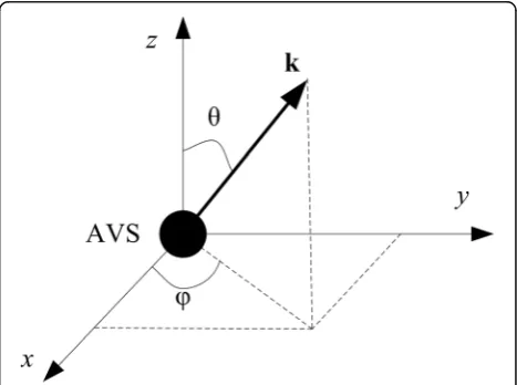
estimation. Figure 1 exhibits the first AVS of the array and the wave vector of one of the impinging signals, which is represented as k, in the Cartesian coordinate system. The density of the water medium ρ and the sound speed in the medium c are assumed to be con-stant and prior known. The AVS array is assumed to be in the far field with respect to all sources, ensuring that the wave fronts at the array are planar.
The acoustic pressure component of the kth source signal at the first sensor of the array is defined as [31]
skð Þ ¼t pkð Þt expð Þiωt ð1Þ
wherepk(t) is a zero-mean complex Gaussian process,
which denotes the slowly varying random pressure enve-lope of the kth source signal. And its variance σ2
k ¼E½ jpkðtÞj
2
denotes the power ofsk(t).
Let a(φk) represent the M-by-1 steering vector, which
is the array’s response to a unit amplitude plane wave from the horizontal direction φk, of an equivalent
pres-sure sensor array, i.e., an array with all of the vector
sensors being replaced by pressure sensors hypothetic-ally. Thus, we have
a φk ¼ 1;e−i2πdcosφk=λ;…;e−i Mð −1Þ2πdcosφk=λ
h iT
ð2Þ
whereλstands for the wavelength. Besides, let uk repre-sent the 4-by-1 response vector of a single AVS to the kth source, which is defined as
uk¼1; cosφk sinθk; sinφk sinθk; cosθkT ð3Þ
The output of the mth sensor at the moment oft is a 4-by-1 vector, which is expressed as
xmð Þ ¼t X K
k¼1
am φk ukskð Þ þt nmð Þt ð4Þ
wheream(φk) denotes themth element ofa(φk), and
nmð Þ ¼t npnvð Þt t ð Þ
ð5Þ
In Eq. (5), np(t) and nv(t) represent the noise of the
acoustic pressure receiver and the particle velocity re-ceiver respectively. Note thatnv(t) is a 3-by-1 vector.
The output of the AVS array is a 4M-by-1 vector by stacking theM4-by-1 measurement vectors of each sen-sor. It can be written as
Xð Þ ¼t xT1ð Þ;t …;xTMð Þt
T
¼½að Þ φ1 u1;…;að Þ φK uKSð Þ þt Nð Þt ð6Þ
where
Sð Þ ¼t ½s1ð Þ;t s2ð Þ;t …;sKð Þt T ð7Þ
contains theKsource signals, and
Nð Þ ¼t nT1ð Þ;t n2Tð Þ;t …;nTMð Þt
T
ð8Þ
Both the signal vector S(t) and the noise vector N(t) are assumed to be independent identically distributed (i.i.d.), zero-mean, complex Gaussian processes. More-over, we assume thatS(t) andN(t) are independent with each other. They can be completely characterized by their covariance matrices
Rs¼ESð ÞSt Hð Þt ¼ diag σ2k ð9Þ
Rn¼ENð ÞNt Hð Þt ¼IM σ 2 p 0 0 σ2vI3
ð10Þ
where σ2p and σ2v represent the variances of the noise of the acoustic pressure receiver and particle velocity re-ceiver respectively, and IM denotes the Mth-order iden-tity matrix.
We define the steering vector of the AVS array, which is represented by ψ(φk) as the Kronecker product of a(φk) anduk. That is to say
ψ φk ¼a φk uk ð11Þ
Thus, Eq. (6) can be rewritten as
Xð Þ ¼t ½ψð Þ;φ1 …;ψð ÞφK Sð Þ þt Nð Þt
¼ΨSð Þ þt Nð Þt ð12Þ
The covariance matrix of the output dataX(t) is
R¼EXð ÞXt Hð Þt ¼ΨRsΨHþRn ð13Þ
3 Method
3.1 Signal cancellation of MVDR beamformer
Without loss of generality, we assume that among theK source signals, one of them is the desired signal, and the others are interference. Let φ~ represent the desired dir-ection, which is unknown and to be estimated.
With regard to the MVDR beamforming method, the problem of solving the optimal weight vector wcan be expressed as
min
w w
HRnw; s:t: wHψð Þ ¼φ 1 ð14Þ
whereφdenotes the view direction, andψðφÞrepresents the corresponding view steering vector. Equation (14) implies that signal from the view direction φ will pass the beamformer without distortion; meanwhile, signals from any other direction will be suppressed.
With the help of the Lagrange multiplier approach,w can be solved as
w¼ R−n1ψð Þφ ψHð ÞRφ −1
n ψð Þφ
ð15Þ
In practice, the noise covariance matrix Rncan hardly
be estimated; therefore, we replace Rnby the estimation
value of the data covariance matrix, which is
^
R¼ 1 N
XN
n¼1
Xð ÞXn Hð Þn ð16Þ
whereNdenotes the number of snapshots.
Given the weight vector w, the beam response of a beamformer is defined as
Hð Þ ¼φ wHψð Þφ ð17Þ
Hð Þφ
j j ¼ ψHð Þφ R^
−1 ψð Þφ
ψHð Þφ R^−1ψð Þφ
ð18Þ
Consider a desired direction-centered angular interval
Φ¼½~φ−Δφ;φ~þΔφ ð19Þ
as the view interval.Δφis a small degree and stands for the radius of Φ. Value of the view direction φ varies within the range ofΦ. If φ≠φ~, the MVDR beamformer would treat the desired signal as an interference signal and suppress it; thus, in the beam pattern of ∣H(φ)∣, there will exist a steep null at the desired direction. This phenomenon is the so-called signal cancellation. On the contrary that ifφ¼φ~, according to the constraint in Eq. (14), ∣H(φ)∣will approximately equal to one within the range ofΦ.
Here, we demonstrate the signal cancellation phenomenon of the MVDR beamformer using a simple computer simulation. Assume thatφ~¼30∘,Δφ= 5∘, and
Φ= [25∘, 35∘]. Let φ be 25∘, 27.5∘, 30∘, 32.5∘, and 35∘ re-spectively. For each value of φ, the beam pattern of
∣H(φ)∣ within the whole horizontal interval [−180∘, 180∘] is plotted in Fig. 2a, where the text “φview” stands forφ. The same beam patterns within the range ofΦare plotted in Fig.2b.
It is evident in Fig. 2b that when φ¼φ~, i.e., 30∘, we have
jHð Þ jφ ≈1; φ∈Φ ð20Þ
However, when φ≠φ~, there are obvious nulls around 30∘in the beam patterns.
This characteristic of the MVDR beamformer can be exploited in finding the desired direction. In the next subsection, the principles of a new DOA estimation al-gorithm is presented.
3.2 DOA estimation
In the case of φ≠~φ, define the minimum of the beam amplitude response ∣H(φ)∣within Φas Hmin, which is
expressed as
Hmin¼ min
φ∈Φ
ψHð ÞφR^−1ψð Þφ ψHð ÞφR^−1ψð Þφ
; φ≠φ~ ð21Þ
According to the previous analysis, as there exists a null withinΦ, thus we have
Hmin≈0 ð22Þ
If φ¼φ~, define the minimum of ∣H(φ)∣ within the intervalΦasH~min, which is expressed as
~
Hmin¼ min
φ∈Φ
ψHð Þφ~ R^−1ψð Þφ ψHð Þφ~ R^−1ψð Þφ~
ð23Þ
According to the previous analysis, we have
~
Hmin≈1 ð24Þ
It can be concluded from Eqs. (22) and (24) that
~
Hmin≫Hmin ð25Þ
Equation (25) indicates that within Φ, if and only if φ ¼~φ, the minimum of the amplitude response reaches the maximum. Since ∣H(φ)∣is determined by the view steering vector, i.e., ψðφÞ, the above necessary and suffi-cient condition is equivalent to the statement that the view steering vector matches the desired steering vector:
ψð Þ ¼φ ψð Þφ~ ð26Þ
We can construct such a worst-case performance optimization problem as
max
φ φmin∈Φ
ψHð ÞφR^−1ψð Þφ ψHð ÞφR^−1ψð Þφ
; s:t:φ∈Φ ð27Þ
In Eq. (27), once the maximum is found, the desired direction is found thereupon. We name this method matched steering vector searching (MSVS) based DOA estimation algorithm.
Equation (27) can be extended to problems involving multiple desired sources. Assume that there areJdesired sources among all the K source signals. For the jth source signal, the desired DOA is~φj, and the view inter-val isΦj¼ ½φ~j−Δφ;φ~jþΔφ, where j= 1,2,…,J. There-fore, the DOA estimation problem for the jth desired signal can be described as
max
φ φmin∈Φj
ψHð ÞφR^−1ψð Þφ ψHð ÞφR^−1ψð Þφ
; s:t:φ∈Φj ð28Þ
Furthermore, the maximum finding problem in Equation (28) can be regarded as a spectrum peak searching prob-lem. We can define the pseudo-spatial power spectrum as
PMSVSð Þ ¼φ min
φ∈Φj
ψHð ÞφR^−1ψð Þφ ψHð ÞφR^−1ψð Þφ
; φ∈Φj ð29Þ
Then, the angles corresponding to the peaks of the spectra are estimation values of the desired directions.
3.3 Algorithm implementation
In practice, to make the view intervals certain, first of all, we shall get the rough estimates of the desired directions using the traditional algorithms such as MUSIC or MVDR. After that, we can establish the view intervals bas-ing on the rough estimates. For the jth view interval Φj,
we sample it uniformly forLsample points and each sam-ple point represents a view direction. The largerLis, the larger the computing load is and the higher the estimation accuracy is. Then, calculate the pseudo-spatial power spectrum according to Eq. (29), and search for the peak to acquire the accurate estimate of the desired direction. The steps of the MSVS algorithm are listed as follows.
3.4 Relation between MSVS and MVDR Algorithm
Given the weight vector w(φ) of a beamformer and the covariance matrix of the output data R, the output power of the beamformer is
Pð Þ ¼φ wHð ÞRwφ ð Þφ ð30Þ
Plug Eq. (15) into Eq. (30), and we can obtain the beam scanning spatial spectrum of the MVDR beamformer:
PMVDRð Þ ¼φ 1
ψHð ÞφR^−1ψð Þφ ð31Þ
In Eq. (31),Rhas been replaced by its estimation value
^
R, which is defined by Eq. (16). Plug Eq. (31) into Eq. (29), and the pseudo-spatial spectrum of the MSVS algo-rithm can be restated as
PMSVSð Þ ¼φ PMVDRð Þφ
min
φ∈Φj
ψHð Þφ R^−1ψð Þφ
;φ∈Φj ð32Þ
Define a window function as
Wjð Þ ¼φ φmin∈Φ
j
ψHð ÞφR^−1ψð Þφ
; φ∈Φj ð33Þ
Then, Eq. (32) can be rewritten as
PMSVSð Þ ¼φ PMVDRð Þ φ Wjð Þ;φ φ∈Φj ð34Þ
Equation (34) indicates that the MSVS pseudo-spatial spectrum can be seemed as the windowed MVDR spatial spectrum. In particular, if WjðφÞ≡1 , the MSVS algo-rithm would turn into the MVDR algoalgo-rithm.
In order to further analyze the performance of the MSVS algorithm, we shall investigate the characteristics of the window functionWjðφÞ.
For the jth desired signal, if φ≠~φj, according to the preceding analysis, the amplitude response will have a null in the direction ofφ~j. Thus, in this case,
Wjð Þ ¼φ ψHð Þφ R^
−1 ψ φ~j
; φ∈Φj; φ≠φ~j ð35Þ
Ifφ¼φ~j, the main lobe of the amplitude response will lie in the view interval Φj. In addition, as Φj is a
rela-tively narrow interval, the amplitude response can be approximately seemed as constant within the range of
Φj. Hence, the window function can be approximately
expressed as
Wjð Þφ ≈ ψH ~φj R^
−1 ψ ~φj
; φ¼φ~j ð36Þ
Wjð Þ ¼φ ψHð ÞφR^ the modulus of the weighted inner product of the view steering vector ψðφÞ and the desired steering vector ψð
~
φjÞ. Here, we present Theorem 1, the proof of which is postponed into theAppendix.
Theorem 1 Assume that N denotes the number of snapshots, M denotes the number of sensors, and N≫M. WjðφÞ ¼ jψHðφÞR^
−1
ψð~φjÞj;φ∈Φj. Then, if and only if φ ¼~φj , the window function WjðφÞ reaches the maximum.
Therefore, the window function WjðφÞ always reach the maximum in the desired direction. Since the MSVS pseudo-spatial spectrum is windowed MVDR spatial spectrum, the peak of the MSVS pseudo-spatial spectrum shall be sharper, and the MSVS algorithm shall have a higher estimation accuracy.
In the next section, we will validate the advantages of the MSVS approach by simulation experiments.
4 Results and discussion
Here, we state some common assumptions. The array is an 8-element uniform linear AVS array. Element spacing d is half-wavelength. There are two source signals im-pinging on the AVS array, and their azimuths are 30∘ and 60∘ respectively. We treat the former signal as the desired signal, whereas the latter as interference. Both signals have equal power. We set the view interval as [25∘, 35∘]. As we only concern on the azimuth estimation, to simplify the problem, assume that for all of the sources, the elevations are 90∘and are pre-known so that the array and the sources are in the same horizontal plane. The angular searching step is 0.1∘.
4.1 Cramer-Rao bound
In the case of a single source, the Cramer-Rao bound (CRB) on the DOA parameters with an AVS array is given in [5]:
p is the ratio of noise powers for the particle velocity receiver and the pressure receiver. If all the noise is in-ternal receiver noise, then ηis a direct reflection of the relative noise floors of the two types of receiver, and the technology is available to make them approximately equal [32], i.e., η= 1. If ambient noise is present, then
η< 1 since the particle velocity receivers filter out some
of the unwanted noise, for example, η= 1/3 for spheric-ally isotropic noise [33]. In order to simulate the under-water environment, we assume that η= 1/3 in the following simulations consistently.
When the origin of the coordinate system is the array centroid,ΓandΠin Eq. (38) are given by
wherermis the position vector of the mth sensor and in unit of wavelength. Assume that the sensors are placed along thex-axis and the array centroid is at the origin of the coordinate system, we have
r1¼ −7
wherehdenotes the direction vector of the source.
CRBð Þ ¼φ 1 2N
1 8ββI 1þ
1 8ββI
21π2sin2φ
4 þ
1 1þη
−1
ð47Þ
4.2 Simulation experiments
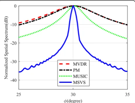
Firstly, we compare the spatial spectra of the proposed MSVS algorithm and some conventional DOA estima-tion approaches, including MVDR, PM, and MUSIC.
Figure3 displays the spatial spectra with SNR = 15 dB andN= 200. In Fig.3, we can find that for all of the four algorithms, there exist clear spectrum peaks around the desired direction, and among them, the proposed one has the sharpest spectrum peak.
The spatial spectra under deteriorated conditions, i.e., SNR =−15 dB andN= 50 are presented in Fig. 4, from which we can find that the spectrum peak of the PM algorithm deviates from the desired DOA seriously. Be-sides, the spatial spectra of MVDR and MUSIC are nearly flat. Unlike these methods, the spatial spectrum of the MSVS algorithm still displays a quite clear peak around 30∘. The 3 dB bandwidth of the MSVS algorithm is much narrower than others. This simulation experi-ment illustrates that the proposed algorithm works effectively even with low SNR and short snapshots. This is due to its sensitivity to the matching degree of the steering vectors. Specifically speaking, when φ deviates fromφ~, the view steering vector mismatches the desired steering vector, and the MSVS spectrum corresponds to the null of the amplitude response within the view inter-val, which is a very small value. However, whenφequals
~
φ, the steering vectors are matched. In this case, the amplitude response within the view interval keeps approximately equalling a large value, causing that the
MSVS spectrum shapes a sharp peak in the desired direction.
Next, we adopt 100 times of Monte Carlo trials to assess the DOA estimation performances of the above-mentioned algorithms. Besides, ESPRIT based on AVS array is put in the comparison. Define the root mean square error (RMSE) as
RMSE¼
ffiffiffiffiffiffiffiffiffiffiffiffiffiffiffiffiffiffiffiffiffiffiffiffiffiffiffiffiffiffiffiffiffiffiffiffi
1 100
X100
m¼1
φ _
m−φ~
2
v u u
t ð48Þ
where _φm stands for the estimate value of the desired DOA in themth Monte Carlo trial.
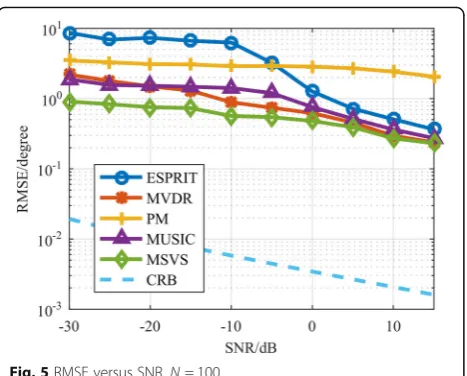
Figure5shows the DOA estimation performance com-parison of the proposed algorithm, ESPRIT, MVDR, PM, and MUSIC approaches, and the CRB under different SNR, with number of snapshots N equals 100. Figure6 depicts the same comparison with different N, and the SNR is fixed on−25 dB.
Figures 5 and 6 illustrate that the performances of all the algorithms degrade with SNR getting lower or N getting smaller. However, it is clearly indicated in both figures that the MSVS algorithm performs better than others under every simulation condition. It can be seen in Fig. 5 that even the SNR is as low as −30 dB, RMSE of the proposed algorithm is less than 1∘. Other algo-rithms cannot achieve such a performance unless the SNR increases at least to about −5 dB. Figure 6 gives similar results.
In the next two experiments, we investigate the anti-interference capability of the MSVS algorithm. In the previous simulations, we assume that the power of the interference signal equals the power of the desired sig-nal, i.e., the interference-to-signal ratio (ISR) is 0 dB. Now, we increase the ISR to 10 dB, 20 dB, and 30 dB
Fig. 3Spatial spectra comparison, SNR = 15 dB,N= 200
successively, with other simulation conditions remaining unchanged. The results are displayed in Fig.7.
Then, we increase the number of the interference sig-nals. In Fig.8,“1 interference”corresponds to the initial assumptions. “2 interferences” means that we add a source signal from the azimuth of 120∘;“3 interferences” for an added source signal from −30∘, and finally “4 in-terferences” for an added source signal from −120∘. All of the ISRs keep to be 0 dB.
Figures 7 and8 illustrate that the performance of the MSVS algorithm is basically independent of the number and intensity of interference. This phenomenon is easy to explain. From the analysis of Section 3, we can see that the MSVS algorithm is essentially a MVDR-based method. Therefore, the MSVS algorithm inherits the strong ability to suppress the interference of the MVDR beamformer.
5 Conclusions
A new DOA estimation algorithm basing on the matched steering vector searching has been presented in this paper. The paper has described the measurement model of an AVS array. After studying on the signal cancellation of the MVDR beamformer, we present our algorithm, introducing its principles and steps to imple-ment. We have also investigated the relation between the proposed algorithm and MVDR method. Then, we conduct the simulation experiments. It is verified that the proposed algorithm has the sharpest spectrum peak and can obtain the best estimation accuracy when com-pared with the conventional DOA estimation algorithms, especially under conditions of low SNR and short snap-shots. What is more, the proposed algorithm has a strong anti-interference capability. The power or num-ber of the interference can hardly affect the performance
Fig. 5RMSE versus SNR,N= 100
Fig. 6RMSE versus number of snapshots, SNR =−25 dB
Fig. 7RMSE with different ISR,N= 100
of our algorithm. In the future, we shall research the joint azimuth angle and elevation angle estimation using the proposed algorithm.
6 Appendix
6.1 Proof of Theorem 1
If the number of snapshots N is large enough, R^ ap-proximately equals R. Thus, Eq. (37) can be rewritten as
Wjð Þ ¼φ ψHð ÞRφ −1ψ φ~j ; φ∈Φj ð49Þ
Firstly, for simplicity, assume that there exists only one source signal, and the desired direction isφ1~ . In this case, the covariance matrix of the output data R1 is expressed as
R1¼σ2
1ψð Þψ~φ1 Hð Þ þ~φ1 Rn ð50Þ
According to Woodbury’s inversion formula, the in-verse ofR1can be expressed as
R−1
In Eq. (52), we represent the constant factor by a capi-talizedC: zero elements being constant, W1ðφÞ reaches the
max-imum if and only if ψðφÞ matches ψðφ~1Þ, i.e., φ equals
~ φ1.
Secondly, assume that there exist two source signals. One is the desired signal, with the azimuth angleφ1~ , and the other is an interference signal with the azimuth angle φ2. In this case, the covariance matrix of the out-put dataR2is expressed as
R2¼R1þσ2
2ψ2ψH2 ð61Þ
By using Woodbury’s inversion formula, the inverse of
R2can be expressed as
R−1
Here, we assume thatφ~1andφ2are far apart, leading the weighted inner product of the corresponding steering vectors to be a very small value, that is
ψH
2CR−n1ψ1~ ≈0 ð65Þ
Plug Eq. (65) into Eq. (63), and we have
W1ð Þφ ≈ψHR−11ψ1~ ð66Þ
Therefore. W1ðφÞ still reaches the maximum if and
areKsource signals, and the interference signals are far apart from the desired signal in direction, the window function would always be expressed byjψHR−1
1 ψ~1j.
This completes the proof of Theorem 1.
Abbreviations
AVS:Acoustic vector sensor; DOA: Direction-of-arrival; ESPRIT: Estimation of signal parameters via rotational invariance technique; i.i.d.: Independent identically distributed; MSVS: Matched steering vector searching;
MUSIC: Multiple signal classification; MVDR: Minimum variance distortionless response; PM: Propagator method; RMSE: Root mean square error; SNR: Signal-to-noise ratio
Acknowledgements
The authors thank the editor and anonymous reviewers for their helpful comments and valuable suggestions. The authors are grateful to the National Science Foundation of China and the National University of Defense Technology for their support of this research.
Author’s contributions
The algorithms proposed in this paper have been conceived by YA, LW, and JWW. YA and LW designed the experiments. YA and KX performed the experiments and analyzed the results. YA is the main writer of this paper. All authors read and approved the final manuscript.
Funding
This research was funded in part by the National Natural Science Foundation of China under grant 61601209 and the Fundamental Research Project of the National University of Defense Technology, under grant
ZDYYJCYJ20140701.
Availability of data and materials
The datasets used and/or analyzed during the current study are available from the corresponding author on reasonable request.
Competing interests
The authors declare that they have no competing interests. And all authors have seen the manuscript and approved to submit to your journal. We confirm that the content of the manuscript has not been published or submitted for publication elsewhere.
Received: 12 June 2019 Accepted: 7 August 2019
References
1. Y. Ao, K. Xu, J.W. Wan, Research on source of phase difference between channels of the vector hydrophone.Proc.IEEE. ICSP., Chengdu, China, 1671– 1676 (2016)
2. P. Felisberto, P. Santos, S.M. Jesus, Tracking source azimuth using a single vector sensor.Proc. Fourth IEEE International Conference on Sensor
Technologies and Application.,Venice, Italy, 416–421 (2010)
3. A. Zhao, X. Bi, J. Hui, C. Zeng, L. Ma, A three-dimensional target depth-resolution method with a single-vector sensor.Sensors18(4), 1182 (2018) 4. A. Nehorai, E. Paldi, Acoustic vector-sensor array processing.IEEE Trans.
Signal Process.42(9), 2481–2491 (1994)
5. M. Hawkes, A. Nehorai, Acoustic vector-sensor beamforming and Capon direction estimation.IEEE Trans. Signal Process.46(9), 2291–2304 (1998) 6. K.T. Wong, M.D. Zoltowski, Closed-form underwater acoustic
direction-finding with arbitrarily spaced vector hydrophones at unknown locations.
IEEE J. Ocean. Eng.22(3), 566–575 (1997)
7. K.T. Wong, M.D. Zoltowski, Root-MUSIC-based azimuth-elevation angle-of-arrival Estimation with uniformly spaced but arbitrarily oriented velocity hydrophones.IEEE Trans. Signal Process.47(12), 3250–3260 (1999) 8. K.T. Wong, M.D. Zoltowski, Self-initiating MUSIC-based direction finding in
underwater acoustic particle velocity-field beamspace.IEEE J. Ocean. Eng. 25(2), 262–273 (2000)
9. M. Hawkes, A. Nehorai, Wideband source localization using a distributed acoustic vector-sensor array.IEEE Trans. Signal Process.57(6), 1479–1491 (2003)
10. H. Chen, J. Zhao, Wideband MVDR beamforming for acoustic vector sensor linear array.IEE Proc. Radar Sonar Navig.151(3), 158–162 (2004)
11. J. He, Z. Liu, Two-dimensional direction finding of acoustic sources by a vector sensor array using the propagator method.Signal Process.88(10), 2492–2499 (2008)
12. Z. Liu, X. Ruan, J. He, Efficient 2-D DOA estimation for coherent sources with a sparse acoustic vector-sensor array.Multidimens. Syst. Signal Process.24(1), 105–120 (2013)
13. K. Han, A. Nehorai, Nested vector-sensor array processing via tensor modeling.IEEE Trans. Signal Process.62(10), 2542–2553 (2014)
14. X. Li, H. Sun, L. Jiang, Y. Shi, Y. Wu, Modified particle filtering algorithm for single acoustic vector sensor DOA tracking.Sensors15, 26198–26211 (2015) 15. W. Si, P. Zhao, Z. Qu, Two-dimensional DOA and polarization estimation for a mixture of uncorrelated and coherent sources with sparsely-distributed vector sensor array.Sensors16, 789 (2016)
16. X. Zhang, M. Zhou, J. Li, A PARALIND decomposition-based coherent two-dimensional direction of arrival estimation algorithm for acoustic vector-sensor arrays.Sensors13, 5302–5316 (2013)
17. J. Li, Q. Lin, C. Kang, K. Wang, X. Yang, DOA Estimation for underwater wideband weak targets based on coherent signal subspace and compressed sensing.Sensors18, 902 (2018)
18. J. Li, Z. Li, X. Zhang, Partial angular sparse representation based DOA estimation using sparse separate nested acoustic vector sensor array.
Sensors18, 4465 (2018)
19. K. Ichige, K. Saito, H. Arai, High resolution DOA estimation using unwrapped phase information of MUSIC-based noise subspace.IEICE Transactions on
Fundamentals of Electronics Communications and Computer Sciences91,
1990–1999 (2008)
20. H. Changuel, A. Changuel, A. Gharsallah, A new method for estimating the direction-of-arrival waves by an iterative subspace-based method.Applied
Computational Electromagnetics Society Journal25(5), 476–485 (2010)
21. Q. Zhao, W.J. Liang, inAdvances in Computer Science, Intelligent System and
Environment. A modified MUSIC algorithm based on eigenspace, vol 104
(Springer Berlin Heidelberg, 2011), pp. 271–276
22. E.A. Santiago, M. Saquib, Noise subspace-based iterative technique for direction finding.IEEE Transactions on Aerospace and Electronic Systems 49(4), 2281–2295 (2013)
23. N. Hu, Z. Ye, D. Xu, A sparse recovery algorithm for DOA estimation using weighted subspace fitting.Signal Processing92(10), 2566–2570 (2012) 24. Q. Xie, Y. Wang, T. Li, Application of signal sparse decomposition in the
detection of partial discharge by ultrasonic array method.IEEE Transactions
on Dielectrics and Electrical Insulation22(4), 2031–2040 (2015)
25. X. Yang, G. Li, Z. Zheng, DOA estimation of noncircular signal based on sparse representation.Wireless Personal Communications82(4), 2363–2375 (2015) 26. K. B. Cui, W. W. Wu, J. J. Huang, X. Chen, and N. C. Yuan,“DOA estimation of
LFM signals based on STFT and multiple invariance ESPRIT,”AEU
-International J Electron Commun, vol.77, pp. 10-17, 2017.
27. B. Widrow, K.M. Duvall, R.P. Gooch, W.C. Newman, Signal cancellation phenomena in adaptive antennas: causes and cures.IEEE Transactions on
Antennas and Propagation30(3), 469–478 (1982)
28. S.A. Vorobyov, Principles of minimum variance robust adaptive beamforming design.Signal Processing93(12), 3264–3277 (2013) 29. J. Li, P. Stoica, Z. Wang, Doubly constrained robust Capon beamformer.IEEE
Transactions on Signal Processing52(9), 2407–2423 (2004)
30. A. Khabbazibasmenj, S.A. Vorobyov, Robust adaptive beamforming for general-rank signal model with positive semi-definite constraint via POTDC.
IEEE Transactions on Signal Processing61(23), 6103–6117 (2013)
31. K.G. Nagananda, G.V. Anand, Subspace intersection method of high-resolution bearing estimation in shallow ocean using acoustic vector sensors.Signal Processing90(1), 105–118 (2010)
32. M.J. Berliner, J.F. Lindberg, O.B. Wilson, Acoustic particle velocity sensors: design, performance and applications.J. Acoust. Soc. America.100(6), 3478– 3479 (1996)
33. G.Q. Sun, D.S. Yang, S.G. Shi, Spatial correlation coefficients of acoustic pressure and particle velocity based on vector hydrophone.Acta. Acustica 28(6), 509–513 (2003)
Publisher’s Note
![Fig. 2 Beam patterns of the beam amplitude responses with different view directions. a In the angular interval of [−180∘, 180∘]](https://thumb-us.123doks.com/thumbv2/123dok_us/907837.1109643/4.595.57.540.566.702/beam-patterns-amplitude-responses-different-directions-angular-interval.webp)