An estimate of the errors of the IGRF/DGRF fields 1945–2000
F. J. Lowes
Physics Department, University of Newcastle, Newcastle upon Tyne, NE1 7RU, U.K.
(Received February 14, 2000; Revised June 3, 2000; Accepted June 19, 2000)
The IGRF coefficients inevitably differ from the true values. Estimates are made of the their uncertainties by comparing IGRF and DGRF models with ones produced later. For simplicity, the uncertainties are summarized in terms of the corresponding root-mean-square vector uncertainty of the field at the Earth’s surface; these rms uncertainties vary from a few hundred to a few nanotesla. (It is assumed that the IGRF is meant to model the long-wavelength long-period field of internal origin, with no attempt to separate the long-wavelength fields of core and crustal origin; the models are meant for users interested in the field near and outside the Earth’s surface, not for core-field theoreticians.) So far we have rounded the main-field coefficients to 1 nT; this contributes an rms vector error of about 10 nT. If we do in fact get a succession of vector magnetic field satellites then we should reconsider this rounding level. Similarly, for future DGRF models we would probably be justified in extending the truncation fromn =10 ton =12. On the other hand, the rounding of the secular variation coefficients to 0.1 nT could give a false impression of accuracy.
1.
Introduction
The IGRF/DGRF is a series of numerical models which approximates the long-wavelength part of the main geomag-netic fieldBof internal origin as it varies with time. It uses a truncated spherical harmonic series to represent the corre-sponding scalar potentialV: here(r, θ, φ)are the usual geocentric spherical polar coordi-nates,ais a reference radius (taken to be the mean radius of the Earth), the Pm
n(cosθ)are Schmidt semi-normalized as-sociated Legendre polynomials, and there are 120 numerical Gauss coefficientsgmn andhmn. (Strictly, it is the magnetic fieldH, unit A/m, which in a source-free region can be repre-sented as the gradient of a scalar potential. However, because all our measurements are in air and water, which have per-meabilityμvery close toμ0, it is conventional to apply (1) to the magnetic flux densityB, unit T; in practice we give the
gm n andh
m
n in units of nT.)
Because the geomagnetic field changes with time—the secular variation—a set of coefficients is specified every 5 years, with linear interpolation used for intermediate times. Because of this secular variation, to derive accurate coef-ficients we need global data coverage for all the relevant epochs. In the absence of such ideal data, the coefficients we estimate are inevitably in error, with the errors being larger at epochs for which the data coverage is poorer.
Copy right cThe Society of Geomagnetism and Earth, Planetary and Space Sciences (SGEPSS); The Seismological Society of Japan; The Volcanological Society of Japan; The Geodetic Society of Japan; The Japanese Society for Planetary Sciences.
This paper discusses how well these numerical coefficients estimate the true values corresponding to the total field of in-ternal origin. It is not concerned with the question of how much of thisn ≤10 internal field comes from crustal mag-netization as opposed to electric currents in the core. Note that the uncertainties quoted by Langelet al.(1989)did in-clude an estimate of the crustal contribution (Sabaka, per-sonal communication, 1997); in effect they treated the IGRF as an estimate of the core field, which the present author thinks was wrong.
What we are really interested in is not the errors in the 120 individual coefficients, but the errorδBin the corresponding magnetic fieldB, whereδBis given by the vector subtraction
δB =BEarth−BIGRF. We will never knowδB; the best we
can hope for is to estimate its magnitude. For a scalar it is usual to express an uncertainty as the root-mean-square error (the standard deviation) to be expected if the analysis were repeated many times using data sets having independent random errors; this concept is easily extended to a vector.
However in our case we have the extra complication that
δB(r, θ, φ)varies in space, as does its standard deviation. Here we will consider the variation only over the Earth’s surface, and quote a single value which is a global root-mean-square vector error, where the mean is taken over r = a. From e.g. Lowes (1966) this is given by taking the square root of paper we will apply (2), using estimates of the standard de-viations of thegm
n andhmn to give the expected rms deviation ofB. But it is important to note that this is an average over
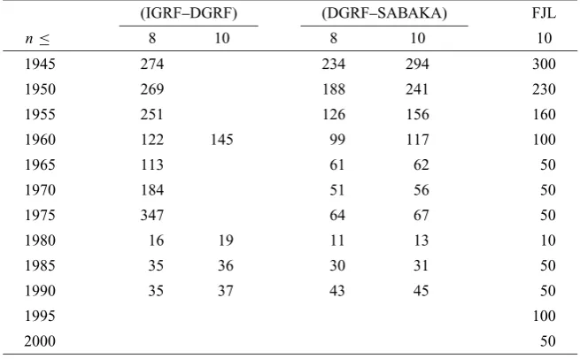
Table 1. Global root-mean-square vector differences between pairs of different models. The second and third columns give the rms differences between the original IGRF and the later DGRF. The fourth andfifth columns give the differences between the DGRF and the continuous spline model of Sabaka et al.(1997). The last column gives the values suggested by Lowes in the IGRF Health Warning (see text).
(IGRF–DGRF) (DGRF–SABAKA) FJL
n≤ 8 10 8 10 10
1945 274 234 294 300
1950 269 188 241 230
1955 251 126 156 160
1960 122 145 99 117 100
1965 113 61 62 50
1970 184 51 56 50
1975 347 64 67 50
1980 16 19 11 13 10
1985 35 36 30 31 50
1990 35 37 43 45 50
1995 100
2000 50
the surface; inevitably, in some regions the actual error will be less than the quotedfigure, while in other regions it will be more, sometimes considerably more. Local errors, par-ticularly in regions with poor data coverage, for example the South Pacific, may well be more than three times larger than the quoted rms value.
We will never know the actual errors of any set of co-efficients; this would involve knowing the true field! The best we can do is to estimate some typical values. Some modellers do try to estimate the standard deviations of their coefficients, based on the lack offit of their model to the data used to produce model. Inevitably this involves a variety of assumptions and interpretations, and in nearly all cases where the proposed standard deviations have been tested in retrospect their values have been found to be too small!
In the next two sections the comparisons between three different sets of models are used to estimate the magnitudes of the errors. The following two sections discuss the effect on the DGRF of rounding errors in the coefficients, and of the truncation, and Section 6 discusses the problem of the secular variation.
2.
Differences Between IGRF and DGRF Models
In most cases the model for a particular epoch is derived in two stages. The production of an IGRF, for an epoch slightly in the future, inevitably involves some forward extrapolation of often inadequate data; we do the best we can, but accept that it may not be very good. Then at a later stage, when we think that we have obtained all the relevant data we are likely to get spanning the epoch, we produce a DGRF model; here the D stands for“definitive”, which does not mean that it is perfect, but that we thought we were unlikely to do significantly better in the future.
So a simple indication of the sorts of errors there were in the IGRF models is to compare them with the correspond-ing (retrospective) DGRF models. This is what is done in columns 2 and 3 of Table 1. There is a complication in that
the earlier IGRFs were produced only up ton = 8, so the second column gives the comparison up ton = 8, and the third column gives the comparison up ton =10 where this is possible.
The large difference for 1975 is because at that time we were feeling our way, and the 1965 IGRF plus secular varia-tion was used for 10 years, rather than for the 5-year period used for all the other epochs. Ignoring that value, we see that the differences vary from about 300 nT rms at 1945 down to about 15 nT at 1980, when at long last we had real global vector data from the MAGSAT satellite; the IGRF 1980 mod-elling was done in 1981, so it included some MAGSAT data. Of course not even the DGRF will be perfect; if the IGRF and DGRF errors were independent, then the differences given in the table would somewhat overestimate the error of the IGRF. However, as much of the data is common to both models, the errors of the models might well be correlated to some extent, so thefigures are not necessarily over-estimates.
3.
Comparison with a Cubic Spline Model
of one third was given to the Sabakaet al.model.)
Of course this Sabakaet al.model has its defects. While the spline constraint allows the good data of 1980 to influence the model at other epochs, there is the possibility that poor data at one epoch will somewhat mar the model elsewhere. (And the covariance matrices for the 5-year epochs will not be independent.) Also the constraint of smoothness in time means that it cannot properly handle geomagnetic jerks. However the Sabakaet al. model is likely to be considerably better than most of the DGRF models. Thefigures of thefifth column of Table 1 are therefore taken as a reasonable estimate of the likely accuracy of the DGRF. This is the basis on which Lowes suggested in 2000 the roundedfigures of the last col-umn as working values in the“IGRF Health Warning”, pub-lished on the IAGA web site athttp://www.ngdc.noaa. gov/IAGA/wg8/igrfhw.html.
4.
Effect of Rounding Errors on DGRF Models
When the IGRF was introduced in 1968 it was correctly thought that the accuracy available then did not justify quot-ing the Gauss coefficients to better than the nearest 1 nT. However this implies a rounding error of up to ±0.5 nT, which contributes a standard deviation of 1/√12=0.3 nT for each coefficient. For ourn≤10 models we see from (2) that this contributes a global rms error of 9 nT. Until now this has been negligible in comparison with the uncertainties of the coefficients, except possibly for 1980 when we had MAGSAT data; at that time the NASA modellers claimed about 1 nT rms error for theirn ≤ 10 model, though the comparison of Table 1 suggests this was too optimistic.
But with the prospect of a succession of vector magne-tometer satellites, such as Ørsted and Champ, we need to think again. Once we have good data, it is perhaps feasible that we can consistently achieve a global model error of a few nT, so for future retrospective DGRF models there is a strong argument that we should specify the coefficients to the nearest 0.1 nT, so as to reduce the rounding error to about 1 nT for an≤10 model.
5.
The Effect of Truncation
Another question that will arise when we have consistently good satellite data is whether the present truncation atn =
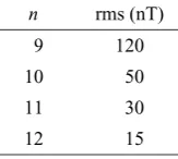
10 is still good enough. Table 2 gives rounded estimates of the contribution of the higher harmonics to the present mainfield. We see that omitting then =11 and 12 terms corresponds to omitting about 35 nT rms, so it would be worth including these terms if the resulting increased error of prediction is significantly less than this value. If in fact we can achieve a few nT vector error for ann ≤10 model, then it is almost certain that this condition would be satisfied. There is therefore a strong case for extending future DGRF models ton =12.
A referee, Dr. De Santis, has pointed out that for mod-els obtained from a non-uniform data set by least squares, and using only a truncated set of coefficients, changing the truncation level could change the amount of higher-harmonic power aliassed into the lower coefficients. However, in the present context, which assumes good coverage of satellite vector data, the actual least-squares’solution is always taken to a higher degree, usually at leastn=13; the truncation to
Table 2. Global rmsfield produced by harmonics of degreen. (Rounded values based on the spectra of Cainet al.(1989), Langel and Estes (1982), and Langelet al.(1989).)
obtain an IGRF occurs onlyafterthe analysis, so no change of aliassing is involved.
6.
The Problem of the Secular Variation
This is the perennial problem of geomagnetic modelling. It has been suggested above that the improved accuracy we can expect will justify changes in the specification of future DGRF models, i.e. in retrospective models for which there is by then good data spanning the relevant epoch. How-ever for future, prospective, IGRF models, the situation is more complicated. The Working Group is now committed to producing such models ahead of time, so some forward extrapolation is necessary, and to estimate the accompanying secular variation will involve even more extrapolation.
The secular variation coefficients, which are applicable for up to 5 years, are at present given to 0.1 nT, so as to give consistency with the 1 nT rounding of the main-field coeffi -cients. However, because we recognize the relatively larger uncertainties involved, we truncate the secular variation co-efficients atn=8, so the consistency is more apparent than real. In fact it is very doubtful if even then=7 and 8
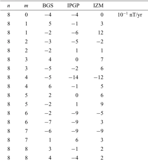
coef-ficients are significant at some epochs. For example, Table 3 gives a comparison of then=8 coefficients of the three sub-missions for the IGRF 2000–2005 secular variation. (Note that for ease of presentation, the coefficient values have been multiplied by 10.) It is clear that for all the coefficients the scatter is far larger than 0.1 nT; in fact in the majority of cases even the average of the three values is not significantly different from zero!
But let us put this into context. By looking at pastfields we can get some feel for the power spectrum of the secular variation, and typical values are given in Table 4. We see that then =7 and 8 terms between them contribute about 5 nT/yr to the secular variation. It is likely that by using these, mostly wrong, coefficients we are at present adding more error than we would by making all the coefficients zero, which is what truncating atn =6 would imply. So for prospective secular variation models based essentially only on surface data (as the three models of Table 3 were) it would probably be more logical to truncate the models atn =6.
From Table 4 we also see that making the n = 9 and 10 coefficients zero is ignoring a contribution of only about 1 nT/yr, so probably does not matter at present. It would mat-ter only if we were able to very much improve the accuracy of then≤8 coefficients.
Table 3. Comparison of secular variation model coefficients. The third, fourth, andfifth columns give then =8 coefficients of the candidate models for IGRF 2000 SV proposed by Macmillan and Quinn (2000), Langlais and Mandea (2000), and Golovkovet al.(2000), respectively.
n m BGS IPGP IZM
Table 4. Power spectrum of the secular variation. The table gives the total global rmsfield produced by terms of degreen.
n rms (nT/yr)
to hope that such satellite data will reduce the errors of the
n =7 and 8 coefficients, so as to make them significant in future models.
But even if the satellite information greatly improves our knowledge of the immediately past secular variation, there is still the problem of extrapolation into the future, as the secular variation itself changes with time at 2–3 nT/yr2, the secular
acceleration. In the past some modellers have used a Tay-lor series in time, incorporating acceleration terms; however these terms are very poorly known, and the series often gives a very poor forecast. More recently, modellers have tried other numerical extrapolation techniques which are perhaps less poor, but it seems likely that the basic problem will re-main until our understanding offluid processes in the Earth’s core allows us to apply some physical constraints to the ex-trapolation.
So what about the prospective IGRF in the golden future when we have plenty of data? Even if a retrospective model
can be determined to a few nT out ton = 12, an IGRF is inevitably going to involve one to two years’forward extrap-olation, which involves using a prospective secular variation model. This will severely degrade the forward-looking IGRF after a few years.
So although the present paper recommends increasing the truncation level for (retrospective) DGRFs ton=12, there is a strong case that, at least for the time being, for the prospec-tiveIGRF we should keep to the present truncation level of
n ≤10 (with coefficients rounded to 1 nT) for the mainfield, andn ≤ 8 (with rounding to 0.1 nT) for the secular varia-tion. The hope is that by doing this we avoid giving less well-informed users too great a confidence in the numbers they are using.
As noted above, the explicit (prospective) IGRF secular variation model will not usually be a good model of the actual time variation then. Similarly, the implicit secular variation involved in the linear interpolation between the (retrospective) 5-year main-field models will not necessar-ily be a good model of the real secular variation then. These
“secular variation”models are there solely to allow extrap-olation/interpolation of the main-field model. Theoreticians should at present look elsewhere for models of the true sec-ular variation.
It is perhapsfitting to end this Section by quoting the fol-lowing, written by Norman Peddie, and presented to the equivalent of Working Group V-8 at the IAGA meeting at Seattle in 1977:
Here lies new IGRF, Had trouble in every nation. He died the way his father died, Of secular variation.
7.
Conclusions
This paper has attempted to quantify the magnitude of the errors in the present sequence of IGRF/DGRF models. The results for the current eighth generation IGRF/DGRF models are summarized by the last column of Table 4.
With reasonable luck, in the near future there should be a succession of vector magnetic survey satellites. The au-thor suggests therefore that the rounding level applied to the DGRF main-field coefficients should be reduced from 1.0 to 0.1 nT, and that the truncation level for the mainfield should be increased fromn=10 ton =12.
On the other hand, for the prospective secular variation the current 0.1 nT/yr rounding, andn =8 truncation, is almost certainly too optimistic at present. The situation should be somewhat better in the future, though we do not yet have proper experience of determining the secular variation from satellite data. However, because of the difficulty of forward extrapolation, the author suggests that it is unlikely that the rounding and truncation levels should be improved beyond their present values.
References
Cain, J. C., Z. Wang, D. R. Schmitz, and J. Meyer, The geomagnetic spec-trum for 1980 and core-crustal separation,Geophys. J.,97, 443–447, 1989.
this issue, 1125–1135, 2000.
Langel, R. A. and R. H. Estes, A geomagneticfield spectrum,Geophys. Res. Lett.,9, 250–253, 1982.
Langel, R. A., R. H. Estes, and T. J. Sabaka, Uncertainty estimates in geo-magneticfield modelling,J. Geophys. Res.,94, 12,281–12,299, 1989. Langlais, B. and M. Mandea, An IGRF candidate main geomagneticfield
model for epoch 2000 and a secular variation model for 2000–2005,Earth Planets Space,52, this issue, 1137–1148, 2000.
Lowes, F. J., Mean-square values on sphere of spherical harmonic vector fields,J. Geophys. Res.,71, 2179, 1966.
Macmillan, S. and J. M. Quinn, The 2000 revision of the joint UK/US geomagneticfield models and an IGRF 2000 candidate model,Earth Planets Space,52, this issue, 1149–1162, 2000.
Sabaka, T. J., R. A. Langel, R. T. Baldwin, and J. A. Conrad, The geo-magneticfield 1900–1995, including the large-scalefield from magneto-spheric sources, and the NASA candidate models for the 1995 revision of the IGRF,J. Geomag. Geoelectr.,49, 157–206, 1997.