Sensor Deployment and Scheduling for Maximizing Energy, Battery Lifetime and Target Coverage in Wireless Sensor Networks

Sensor Deployment and Scheduling for Maximizing

Energy, Battery Lifetime and Target Coverage in

Wireless Sensor Networks

Nikhil Nagpure

, Siddhesh Wadekar

, Sanket Mote

, Prof. Sumitra Sadhukhan

Email: [email protected], [email protected] 2

,[email protected],[email protected]

Abstract-In this paper, we have work on the enhancement of sensor lifetime in the sink of sensor networks. The

main objectives are determining the quality of services of the network and maximize the battery lifetime. The problem of estimating redundant sensing areas among neighbouring sensors is analysed. We present simple methods to estimate the redundancy without the knowledge of the location or directional information. Energy usage must be restricted to attain improved lifetime of the sensor. The primary objective of this work is sensor deployment under optimal location with enhanced network lifetime. The secondary objective is to schedule sensor nodes with highest possible lifetime and maximum efficiency. This paper solves the coverage problem with a maximizing lifetime in wireless sensor nodes.

Index Terms-Wireless Sensor Scheduling, Battery Lifetime, Sensor Deployment, Coverage Problem, Energy

Efficient

1. INTRODUCTION

Wireless Sensor Networks (WSN) can be considered a particular type of Mobile Ad-hoc Network (MANET), formed by hundreds or thousands of sensing devices communicating by means of wireless transmission in a respective sink. Research on WSNs and MANETs share similar technical problems. Consequently, simulation is essential to study WSN, being the common way to test new applications and protocols in the field. This fact has brought a recent boom of simulation tools available to model WSN.

Similarly, implementing a complete model requires a considerable effort. A tool that helps to build a model is needed and the user faces the task of selecting the appropriate one. Simulation software commonly provides a framework to model and reproduce the behavior of real systems. However, actual implementation and “secondary goals” of each tool differ considerably, that is, some may be designed to achieve good performance and others to provide a simple and friendly graphical interface or emulationa1 capabilities. The objective of this contribution is to present an extensive survey on experimental tools especially used for WSN research purposes that are based on various criteria, scenario conditions, parameters and other factors, also presenting the other relevant contents related to experimental tools, as well as focusing on the highly summarized merits and demerits of mostly presented experimental tools with respect to WSNs.

One of the main issues faced in the deployment techniques of WSNs is to target the areas where the sensors will be deployed in order to fetch the real-time data for analysis as per the requirements efficiently, this phenomenon is also referred as target coverage problem. Another issue is to maximize the battery life of the wireless sensor networks we have implemented heuristic approach scheduling algorithm in order to function only required wireless sensors in the particular area in order to maximize the battery life of the WSNs respectively. Basically, coverage problem can be divided as area coverage problem and target coverage problem. In area coverage, the main focus is on monitoring the whole region of interest, in other hand target coverage focuses on monitoring only specific points in a given region. Target coverage further classified as simple coverage, k-coverage, and Q-coverage.

In simple coverage, each sensor node should be monitoring, at least, one target area. In k-coverage, k sensor node should be monitoring each target area. Here k is a predefined integer constant. But in Q-coverage, suppose there are n a number of the target area(T) and the same number of the sensor node, then, at least, one sensor node should be monitoring, at least, one target area. Basically, using Sensor Deployment and sensor scheduling we achieved a solution for coverage problem. There are two traditional ways for sensor deployment i.e. Random deployment and Deterministic deployment. Apart from this, there are several algorithms which are used for sensor deployment for solving optimization

problems. Similarly, there are several ways of computing deployment locations. Bio-inspired algorithms

prove to be effective for solving optimization problems.

2. PROBLEM STATEMENT

In the previous case of wireless sensor networks the main issue observed was the battery lifetime of the sensors which on complete analyzing we found heuristic approach algorithm can be used for scheduling of sensor networks and only required sensors will be turned on when required rest other sensors will be in sleep mode and in this way the maximum region under the sink will be sensed respectively. Similarly, the other main issue observed was the deployment of the wireless sensor networks in the targeted coverage area therefore, we can use the artificial bee colony algorithm and particle swarm optimization algorithm in order to deploy the sensors in the targeted area from where they can cover the maximum area for sensing and collecting the real-time information respectively. The objective is to deploy the sensor nodes such that the network lifetime is maximum and to schedule the sensor nodes so as to achieve the optimal network lifetime. To achieves this two objects, the first phase, we need to find out Upper Bound of network lifetime using coverage matrix.

Consider m no of sensor {S1, S2, ..., Sm} are placed for deployment process in Area R. In Area R, there are n no of target {T1, T2, …, T

= 1,_{0, ℎ}

Eq. (1)

where i= 1, 2, . . ., m and j = 1, 2, . . ., n.

We define bi= bi/ei to denote the lifetime of battery, where bi is the initial battery power and ei is the energy consumption rate of Si. The upper bound is the maximum achievable network lifetime for a particular configuration, the upper bound is calculated as,

= ∑ Mij ∗ bi _! " Eq. (2)

For k-coverage, q j = k, j = 1, 2, . . ., n.

Second think need to solved coverage problem. The coverage problem can be classified into k-coverage &Q-coverage which is as follows:

2.1.k-Coverage deployment and Scheduling

Given a set of sensor nodes S = {S1, S2, . . ., Sm} with battery power B = {b1, b2, . . ., bm}, energy consumption rate Ei for Siand a target set T = {T1, T2, . . ., Tn}, place the nodes such that each target is monitored by at least k-sensor nodes and to maximize

U. generate a schedule {C1, . . ., Cy}, for {t1, . . ., ty}, such that for all ticks,

• each target is covered by at least k sensor nodes, 1≤k≤m

• network lifetime ∑tpis maximized.

2.2.k-Coverage deployment and Scheduling

Given a set of sensor nodes S = {S1, S2, . . ., Sm} with battery power B = {b1, b2, . . .,bm}, energy consumption rate Ei for Si and a target set T = {T1, T2, . . .,Tn}, place the nodes such that each target Tj, 1 ≤ j ≤ n, is covered by at least qj sensor nodes and to maximize U. generate a schedule {C1, . . ., Cy}, for {t1, . . .,ty}, such that for all ticks,

• T = {T1, T2, . . ., Tn} is covered by at least Q= {q1, q2, . . ., qn} sensor nodes, where each target Tj, 1 ≤ j ≤ n, is covered by at least q j sensor nodes

• network lifetime ∑tp is maximized.

3. EXISTING METHOD

In the existing system, they use Artificial Bee Algorithm (ABC Algorithm), Particle Swarm Optimization (PSO Algorithm) and heuristic algorithm for Sensor Deployment to compute sensor deployment location. And heuristic algorithm for Sensor Scheduling to maximize the battery lifetime.

4. PROPOSED METHOD

Sensor nodes are placed randomly; the deployment locations and schedule are decided at the base station according to the deployment of sensors. In this proposed approach, there are two phases: the first phase is sensor deployment and the second phase is sensor scheduling. In the first phase of sensor deployment, we have used artificial bee colony algorithm and particle swarm optimization. Also in the second phase for sensor scheduling, we have used the heuristic algorithm.

4.1.

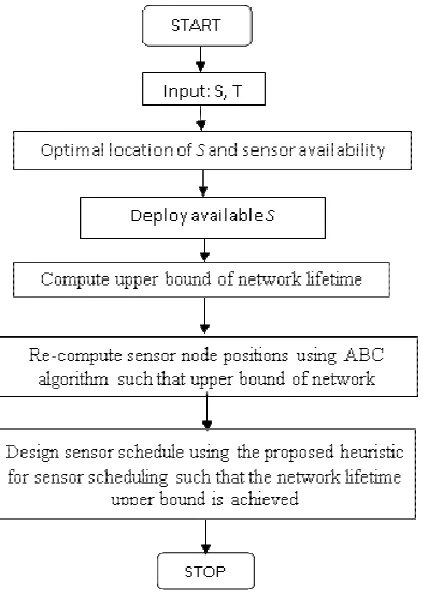
4.2.Flowchart

4.3.Sensor Deployment:

4.3.1.Artificial bee colony algorithm for Sensor Deployment

Artificial Bee Colony (ABC) is one of the most popular swarm intelligence algorithms introduced by DervisKaraboga in 2005, motivated by the intelligent behavior of honey bees. It is as simple as Particle Swarm Optimization (PSO) and Differential Evolution (DE) algorithms. ABC as an optimization tool provides a population-based search procedure in which individuals called foods positions are modified by the artificial bees with time and the bee’s aim is to discover the places of food sources with high nectar amount and finally the one with the highest nectar. In ABC system, the model consists of three essential parts: employed and unemployed foraging bees, and food sources. The first two components, employed and unemployed foraging bees, search for rich food sources, which is the third part, close to their hive. artificial bees fly around in a multidimensional search space and some (employed and onlooker bees) choose food sources depending on the experience of

Figure 1Flowchart

colony algorithm for Sensor

Artificial Bee Colony (ABC) is one of the most popular swarm intelligence algorithms introduced by DervisKaraboga in 2005, motivated by the intelligent behavior of honey bees. It is as simple as Particle ation (PSO) and Differential Evolution (DE) algorithms. ABC as an optimization based search procedure in which individuals called foods positions are modified by the artificial bees with time and the bee’s aim is to places of food sources with high nectar amount and finally the one with the highest nectar. In ABC system, the model consists of three essential parts: employed and unemployed foraging bees, and food sources. The first two components, employed ed foraging bees, search for rich food sources, which is the third part, close to their hive. artificial bees fly around in a multidimensional search space and some (employed and onlooker bees) choose food sources depending on the experience of

themselves and their nestmates and adjust their positions. Some (scouts) fly and choose the food sources randomly without using experience. If the nectar amount of a new source is higher than that of the previous one in their memory, they memorize the new position and forget the previous one. Thus, ABC system combines local search methods, carried out by employed and onlooker bees, with global search methods, managed by onlookers and scouts, attempting to balance exploration and exploitation process.

Theorem 4.1. ABC Algorithm

1: Initialize the solution population 2: Evaluate fitness

3: cycle = 1 4: repeat

5: Search for new solutions in the neighborhood 6: if new solution is better than old solution 7: Memorize new solution and discard old solution 8: end if

9: Replace the discarded solution with a new randomly generated solution

10: Memorize the best solution

205 and their nestmates and adjust their positions. Some (scouts) fly and choose the food sources randomly without using experience. If the nectar amount of a new source is higher than that of the previous one in their memory, they memorize the d forget the previous one. Thus, ABC system combines local search methods, carried out by employed and onlooker bees, with global search methods, managed by onlookers and scouts, attempting to balance exploration and exploitation

Algorithm 1: Initialize the solution population B

5: Search for new solutions in the neighborhood new solution is better than old solution then 7: Memorize new solution and discard old solution

Replace the discarded solution with a new randomly generated solution

206

11: cycle = cycle + 1

12: until cycle = maximum cycles

4.3.2. Particle Swarm Optimization algorithm for Sensor Deployment

Particle Swarm Optimization (PSO) is a robust optimization technique based on the movement and intelligence of swarms. It was introduced by James Kennedy (social-psychologist) and Russell Eberhart (electrical engineer) in 1995. The basic idea of Particle Swarm Optimization is following: Each particle is searching for the optimum. Each particle is moving and hence has a velocity. Each particle remembers the position it was in where it had its best result so far (its personal best). But this would not be much good on its own; particles need help in figuring out where to search. The particles in the swarm co-operate. They exchange information about what they’ve discovered in the places they have visited. gbest locations, with a random weighted acceleration at each time step.

Particle position is affected by velocity. Assume xi(t) is particle I position at time t; unless otherwise stated, t is discrete time. The position of the particle is

3: for each particle do 4: Calculate the fitness value

5: if fitness value is better than the best fitness value (pbest) in history then

6: Set current value as the new pbest 7: end if

8: end for

9: Choose the particle with the best fitness value of all the particles as the gbest

10: for each particle do

11: Calculate particle velocity according to velocity update equation (4)

12: Update particle position according to position update equation (3)

13: end for

14: until maximum iterations or minimum error criteria is attained

4.4.Sensor Scheduling

4.4.1. Heuristic algorithm for Sensor Deployment

The term heuristic is used for algorithms which find solutions among all possible ones, but they do not guarantee that the best will be found, therefore they may be considered as approximately and not accurate algorithms. These algorithms, usually find a solution close to the best one and they find it fast and easily. Sometimes these algorithms can be accurate, that is they actually find the best solution, but the algorithm is still called heuristic until this best solution is proven to be the best. The method used by a heuristic

2: Initialize k/Q, max_run, priority calculated using battery power

3: for r = 1 to max_rundo 4: for iteration = 1 to m i=1 bi do 5: if cover possibility exists then 6: Determine cover based on priority 7: Optimize cover

8: Activate optimized cover and reduce battery power 9: else

10: break 11: end if 12: end for

13: Calculate network lifetime (nlife) 14: if nlife< U then

15: Consider weight due to covered targets to compute priority to check for better lifetime 16: else

5.RESULTS

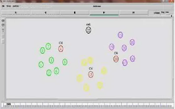
We consider a 500 m × 500 m region for experiments. The number of targets is 25. The number of sensor nodes (m) is varied from 100 to 250. Sensing range of each sensor node is fixed as 75 m. In random deployment, there is more chance of targets being not detected or targets not being covered with the required level of coverage. However, this may not hold true with the dense deployment of nodes. But there is another possibility

Fig 2. Sensing of data from active Sensors in Sink. We consider a 500 m × 500 m region for

experiments. The number of targets is 25. The number of sensor nodes (m) is varied from 100 to 250. Sensing range of each sensor node is fixed as 75 m. In random deployment, there is more chance of etected or targets not being covered with the required level of coverage. However, this may not hold true with the dense deployment of nodes. But there is another possibility

of some targets being monitored by many sensor nodes, and some by a few sensor no

difference in the number of sensor nodes monitoring each target will affect the network lifetime. The sensor nodes may be positioned in a better way so as to avoid this variation. This will yield better lifetime. Though random deployment has thes

there are applications where random deployment is the only feasible strategy.

Fig 1. Deployment of Sensors in Sink.

Fig 2. Sensing of data from active Sensors in Sink.

6. FUTURE WORK:

We plan to extend this method of deployment and scheduling for probabilistic coverage in wireless sensor networks. Since this method aims at maximizing the battery lifetime of the wireless networks it is cheaper and profitable to install the sensor networks for a maximum period of time respectively.

7. CONCLUSIONS

In this paper, we compute deployment locations of the wireless sensor nodes using heuristic approach for scheduling and geometric approach for

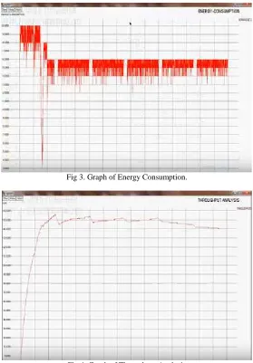
Fig 3. Graph of Energy Consumption.

Fig 4. Graph of Throughput Analysis

We plan to extend this method of deployment and scheduling for probabilistic coverage in wireless sensor networks. Since this method aims at maximizing the battery lifetime of the wireless sensor networks it is cheaper and profitable to install the sensor networks for a maximum period of time

In this paper, we compute deployment locations of the wireless sensor nodes using heuristic approach etric approach for

deploymentsuch that the network lifeti maximum respectively.

In the previous paper Artificial Bee Colony algorithm is used for scheduling of the wireless nodes we analyzed Heuristic approach algorithm computes and performs better than the Artificial Bee Colony for this problem. In order to avoid the battery drain of all wireless nodes at a respective time, sensor nodes scheduling can be done so that a minimum number of sensor nodes required for satisfying the coverage needs to be turned on, by using heuristic approach algorithm other nodes can be reserved for the later use. Therefore, we can extend the lifetime of the network using the deployment algorithm i.e. geometric approach respectively.

208 deploymentsuch that the network lifetime is

209

8. REFERENCES

[1] S. Mini, Siba K. Udgata, and Samrat L. Sabat,“Sensor Deployment and Scheduling for Target Coverage Problem in Wireless Sensor Networks”, IEEE Sensors Journal, Vol. 14, No. 3, March 2014.

[2] J. Wang, R. Ghosh, and S. Das, “A survey on sensor localization,” J. Control Theory Appl., vol. 8, no. 1, pp. 2–11, 2010.

[3] C.-F. Huang and Y.-C. Tseng, “The coverage problem in a wireless sensor network,” in Proc. 2nd ACM Int. Conf. Wireless Sensor Netw. Algorithms simulating bee swarm intelligence,” Artif. Intell. Rev., vol. 31, nos. 1–4, pp. 61–85, 2009.

[6] D. Karaboga and B. Basturk, “On the performance of the artificial bee colony (ABC) algorithm,” Appl. Soft Comput., vol. 8, pp. 687– 697, Jan.2008.

[7] D. Karaboga, B. Gorkemli, C. Ozturk, and N. Karaboga, “A comprehensive survey: Artificial bee colony (ABC) algorithm and applications,”Artif. Intell. Rev., 2012, pp. 1–37. 644 IEEE SENSORS JOURNAL, VOL. 14, NO. 3, MARCH 2014

[8] J. Yick, B. Mukherjee, and D. Ghosal, “Wireless sensor network survey,” Comput. Netw., vol. 52, pp. 2292–2330, Aug. 2008. [9] K. Wu, Y. Gao, F. Li, and Y. Xiao,

“Lightweight deployment-aware scheduling for wireless sensor networks,” Mobile Netw. Appl., vol. 10, pp. 837–852, Dec. 2005.

[10]X. Bai, S. Kumar, D. Xuan, Z. Yun, and T. H. Lai, “Deploying wireless sensors to achieve both coverage and connectivity,” in Proc. 7th ACM Int. Symp. Mobile Ad Hoc Netw. Comput., 2006, pp. 131–142.

[11]C. Liu, K. Wu, and V. King, “Randomized coverage-preserving scheduling schemes for wireless sensor networks,” in Proc. Netw., 2005, pp. 956–967.

[12]C.-Y. Chang and H.-R. Chang, “Energy-aware node placement, topology control and MAC scheduling for wireless sensor networks,” Comput. Netw., vol. 52, pp. 2189–2204, Aug.

“Artificial bee colony algorithm for dynamic deployment of wireless sensor networks,” Turkish J. Electr. Eng. Comput. Sci., vol. 20, no. 2, pp. 255–262, 2012.

[15]S. K. Udgata, S. L. Sabat, and S. Mini, “Sensor deployment in irregular terrain using artificial bee colony algorithm,” in Proc. World Congr. Nature Biol. Inspired Comput., Dec. 2009, pp. 1309–1314.

[16]S. Mini, S. K. Udgata, and S. L. Sabat, “Artificial bee colony based sensor deployment algorithm for target coverage problem in 3-D terrain,” in Proc. Distrib. Comput. Internet Technol., 2011, pp. 313–324.

[17]S. Mini, S. K. Udgata, and S. L. Sabat, “A heuristic to maximize network lifetime for target coverage problem in wireless sensor networks,” Ad- Hoc Sensor Wireless Netw., vol. 13, nos. 3–4, pp. 251–269, 2011.

[18]J. Riley, U. Greggers, A. Smith, D. R. Reynolds, and R. Menzel, “The flight paths of honeybees recruited by the waggle dance,” Nature, vol. 435, pp. 205–207, Mar. 2005.

[19]J. Kennedy and R. Eberhart, “Particle swarm optimization,” in Proc. IEEE Int. Conf. Neural Netw., vol. 4, Nov./Dec. 1995, pp. 1942–1948. [20]R. Eberhart and J. Kennedy, “A new optimizer

using particle swarm theory,” in Proc. 6th Int. Symp. Micro Mach. Human Sci., Oct. 1995, pp. 39–43.

[21]Dian PalupiRini, SitiMariyamShamsuddin, SitiSophiyatiYuhaniz, “Particle Swarm Optimization: Technique, System, and Challenges”, International Journal of Computer Applications (0975 – 8887) Volume 14– No.1, January 2011.