Essays on Information Collection

(1)

Essays on Information Collection

Thesis by

Tatiana Mayskaya

In Partial Fulfillment of the Requirements for the Degree of

Doctor of Philosophy

CALIFORNIA INSTITUTE OF TECHNOLOGY Pasadena, California

2017

(2)

(3)

ACKNOWLEDGEMENTS

I thank Benjamin J. Gillen for guiding me through my time in graduate school with his constant support. I would not have made it without him.

For my job market paper in Chapter2, I am grateful to Federico Echenique, Jakša Cvitanić, Jean-Laurent Rosenthal, Marina Agranov, Alexander V. Hirsch, Leeat Yariv, Luciano Pomatto, Kim C. Border, Omer Tamuz and Michael Ewens for many productive discussions and helpful suggestions. I also thank Welmar E. Rosado-Buenfil, Marcelo A. Fernández, Lucas Núñez, and Myungkoo Song for numerous useful comments and Yilmaz Kocer and Juuso Toikka for providing relevant literature references.

For the experimental project in Chapter 3, I am grateful to Charles R. Plott for inspiration, guidance and constant support. I am also indebted to Alexis V. Belianin and Fuad T. Aleskerov for their help in running experiments in the Laboratory for Experimental and Behavioral Economics at the High School of Economics in Moscow.

(4)

ABSTRACT

This thesis is devoted to the problem of information collection from theoretical and experimental perspectives.

In Chapter 2, I characterize the unique optimal learning strategy when there are two information sources, three possible states of the world, and learning is modeled as a search process. The optimal strategy consists of two phases. During the first phase, only beliefs about the state and the quality of information sources matter for the optimal choice between these sources. During the second phase, this choice also depends on how much the agent values different types of information. The information sources are substitutes when each individual source is likely to reveal the state eventually, and they are complements otherwise.

In Chapter3, co-authored with Li Song, we conducted an experiment which demon-strates that even in a simple four person circle network people appear to fail to account for possible repetition of information they receive. Moreover, we show that this phenomenon can be partially attributed to rational considerations, which take into account other people’s deviations from optimal behavior.

(5)

LIST OF ILLUSTRATIONS

Number Page

2.1 Illustration for Theorem 1, Case 1 and Case 2 . . . 20

2.2 Illustration for Theorem 1, Case 3 . . . 21

2.3 Illustration of the optimal strategy when the probability of state 3 is zero . . . 24

2.4 Illustration for Theorem 2 . . . 27

2.5 Illustration of the optimal strategy when only one source is available . 28 2.6 Example of the optimala-type strategy . . . 31

2.7 Illustration for Theorem 3, Case 1. . . 34

2.12 Example of the optimal strategy . . . 41

2.13 Illustration for Theorem 4 . . . 43

3.1 The network structure applied in the experiment . . . 57

3.2 Profit distribution . . . 59

3.3 Guess distribution . . . 59

3.4 Guess distribution by periods . . . 60

4.1 Functions f(ρ)and f0(ρ) . . . 84

4.2 Function ρf0(ρ) . . . 86

4.3 Functionsh0(c)andch0(c) . . . 86

A.1 Optimala-type strategy for Case 2 . . . 115

A.2 Optimala-type strategy for Case 3 . . . 116

A.3 Optimala-type strategy for Case 4, partition based on immediate action121 A.4 Optimala-type strategy for Case 4, partition based on future strategy 123 A.5 Optimala-type strategy for Case 5, partition based on immetiate action126 A.6 Optimala-type strategy for Case 5, partition based on future strategy 127 A.7 Optimal a-type strategy for Case 6.1, partition based on immediate action . . . 139

(8)

A.9 Optimal a-type strategy for Case 6.3, partition based on immediate

action . . . 141

A.10 Optimala-type strategy for Case 6.1, partition based on future strategy142 A.11 Optimala-type strategy for Case 6.2, partition based on future strategy143 A.12 Optimala-type strategy for Case 6.3, partition based on future strategy144 A.13 Optimala-type strategy for Case 7, partition based on immediate action148 A.14 Optimala-type strategy for Case 7, partition based on future strategy 149 A.15 The partition of the space(R1,R2)into Cases 1-7 when _cc1λ2₂_λ₁ =2. . . . 150

B.1 The distribution of the balls . . . 166

B.2 The network . . . 167

B.3 Screenshot . . . 169

B.6 Equilibrium data, stage 2 . . . 180

B.7 Equilibrium data, stage 3 . . . 181

(9)

LIST OF TABLES

Number Page

3.1 Estimation for pooled data . . . 62

3.2 Subject classification . . . 66

3.3 Performance on PBH-fit . . . 68

3.4 Subject classification based onIdeal Guess . . . 69

3.5 PBH-fit real on PBH-fit ideal. . . 71

A.1 Proof of Theorem 3. Step 3. . . 153

B.1 Model fit for different specifications (pooled data) . . . 175

B.2 Equilibrium fit . . . 179

B.3 Model fit for different specifications (Session 1) . . . 183

B.9 Performance on PBH-fit (stages 1,2,3 and 4) . . . 189

B.10 Performance on PBH-fit (all stages) . . . 190

B.11 Performance on PBH-fit (stages 3,4 and 5) . . . 191

B.12 Performance on PBH-fit (stages 3 and 4) . . . 192

B.13 Performance on PBH-fit (stage 3) . . . 193

B.14 Performance on PBH-fit (stages 1,2 and 3) . . . 193

B.15 Performance on PBH-fit (stages 4 and 5) . . . 194

B.18 Model fit for different specifications (pooled data, based on Ideal Guess) . . . 196

B.19 Model fit for different specifications (Session 1, based onIdeal Guess)197 B.20 Model fit for different specifications (Session 2, based onIdeal Guess)198 B.21 Model fit for different specifications (Session 3, based onIdeal Guess)199 B.22 Model fit for different specifications (Session 4, based onIdeal Guess)200 B.23 Model fit for different specifications (Session 5, based onIdeal Guess)201 B.24 Model fit for different specifications (Session 6, based onIdeal Guess)202 B.25 PBH-fit real on PBH-fit ideal for different specifications (Part I) . . . 203

(10)

C h a p t e r 1

INTRODUCTION

In this thesis, I address several questions related to dynamics and results of the learning process. Chapter 2gives an abstract framework for studying dynamically optimal information collection from multiple information sources. Chapter 3 ex-plores learning in a network setting using experimental economics tools. Chapter4 provides a theoretical background for overconfidence in learning.

In Chapter2, I consider the situation in which a decision maker has two sources of information that she can choose to use. She is free to change the source as often as she wants as she collects information about a payoff relevant state. Each source is modeled as a search process for the proof that a certain state is realized. There are three possible state realizations, with two that are possible to verify through information sources. In the optimum, the decision maker starts with searching for the most likely out of the two verifiable states (adjusted to how easy and how costly it is to search for a given state), switching attention as she becomes more pessimistic about the state. Then at some point she changes her learning behavior to focusing on only one source until she either finds the true state or gives up the attempt to learn completely.

(11)

(12)

C h a p t e r 2

DYNAMIC CHOICE OF INFORMATION SOURCES

2.1 Introduction

There are many situations where an individual has the opportunity to use different sources to gather costly information before choosing among a set of alternatives. When the individual can change information sources as often as he wants, finding his optimal behavior is difficult both as a theoretical and a computational exercise. I propose a tractable way to model this problem and derive its solution.1 I characterize a unique optimal information collection strategy when there are two information sources and three possible states of the world. The optimal strategy consists of two phases. During the first phase, the optimal choice of an information source depends only on the precision and cost of information and the agent’s current beliefs about the state of the world. In this phase, the best source is the one that reveals the state most quickly, which may guide the agent to alternate between sources. During the second phase, the best choice also depends on the payoff the agent receives from choosing among the set of alternatives after the learning process. However, during this phase, the agent never alternates between sources.

This characterization of the optimal strategy can be used to deliver new insights into the market of information providers by determining when the information sources are substitutes and when they are complements. I show that sources act as substitutes when ex ante it is very likely that, given all potential information from one source, the other source cannot contribute anything new, and they are complements otherwise.

In my model, the agent must choose one of three alternatives. The payoff the agent receives from each alternative depends on the true state of the world. There are three possible states. Before making a choice, the agent can collect information about the true state from two sources. The information collection process is modeled in

1_{Che and Mierendorff (2016) independently develop a very similar approach with two main}

(13)

continuous time to allow the agent maximal freedom in allocating his attention. At every instant, the agent can either stop information collection by choosing an alter-native that maximizes his current expected utility or wait and get more information. If he wants more information, he must choose how to allocate a unit of his attention between two sources (source 1 and source 2). If a source receives a positive amount of attention, the agent observes a signal from this source and he has to pay a cost proportional to the amount of attention he pays to this source.2,3 If the world is in statei (i = 1,2), then sourcei sends a positive signal with probability proportional to the source intensity and attention paid to this source; otherwise the signal is 0. If the world is not in statei, then sourceisends signal 0 all the time.

My main result describes the unique optimal information collection strategy.4 Once the agent observes a positive signal, the true state is revealed and therefore the agent stops the information collection process. Conditional on receiving only 0 signals, the agent chooses what source to use and when to stop seeking additional information according to a rule defined by two thresholds. Until the agent’s beliefs about the state reach the first threshold, he chooses the source that is informatively optimal (I call it the informatively optimal phase of the information collection process). Between the two thresholds, he chooses the payoff optimal source (the payoff optimal phase). Once his beliefs reach the second threshold, he stops collecting information.

During the informatively optimal phase, the agent compares the quality of both sources and chooses the one with the highest quality as measured by the ratio of the probability of receiving a positive signal from this source to the cost of observing this signal. Since new information changes the agent’s beliefs about the true state, it also changes the probability of receiving a positive signal from each source. Thus, the quality of the sources changes as the agent gets more signals. The more 0 signals the agent gets from a given source, the lower the probability of receiving a positive signal from this source and the higher the probability of receiving a positive signal from the other source. Therefore, observing a signal of 0 lowers the quality of this source

2_{I assume the cost only depends on the type of source, so that it is independent of the true state}

and the agent’s payoff from different alternatives. For example, it can be money a researcher pays to subjects of experiments or it can be a constant fee to an expert.

3_{Moscarini and Smith (2001) introduce a discounting and time-dependent information cost for}

the optimal experimentation model with one information source. My model serves as a benchmark for such modifications when there are two information sources.

4_{Strictly speaking, the optimal strategy is unique in the following sense. The strategy is}

(14)

and raises the quality of the other source. At the beginning of the informatively optimal phase, the agent starts with the source that has the highest quality. As phase one progresses, the quality of that source decreases while the quality of the other source increases. Given enough 0 signals, the qualities equalize, at which point the agent starts using both sources simultaneously by splitting his attention between two sources. Moreover, by paying more attention to the source with low intensity, the agent guarantees that the qualities stay equal after new information is received.

At the payoff optimal phase, the agent uses a constant attention allocation plan that places full attention to either source 1 or source 2. At the beginning of this phase, the agent chooses the source that gives him the highest expected payoff and then he stays with this source until the end of the information collection process. The payoff optimal phase illustrates an “elimination search” behavior. The optimal information source during this phase is sometimes that with the lowest probability of producing a positive signal. Put simply, it is sometimes optimal to search in a place where you do not think you are going to find something in order to eliminate this place.

Both thresholds that define the optimal strategy occur where the marginal cost of information equals its marginal benefit. Consider the second threshold that indicates where the payoff optimal phase ends and suppose that source 1 is used during this phase. Here, the marginal cost of information is the cost of a signal from source 1 and the marginal benefit is the expected change in the payoff from the chosen alternative. This change in payoff is positive only if the received signal is positive; otherwise, this change would be zero. Thus, the marginal benefit is the probability of receiving a positive signal from source 1 multiplied by the difference between the payoffs in state 1 from the alternatives the agent would choose after receiving a positive signal from source 1 and after receiving signal 0 from that source. I call this benefit a direct benefit since it is directly related to the final payoff.

(15)

that source. This part accounts for the benefit from a positive signal. The indirect benefit comes from signal 0 and it reflects the increase in the direct benefit from all future signals the agent is going to receive from source 1 during the payoff optimal phase. Indeed, signal 0 from source 2 makes the agent more optimistic about state 1, therefore increasing the likelihood of getting a positive signal from source 1.

I use the characterization of the optimal learning strategy to find when the infor-mation sources complement each other and when they substitute for each other. I call two sources complements if raising the cost of a signal from one source leads to a lower expected attention allocated to the other source during the information collection process. I call two sources substitutes if raising the cost of a signal from one source leads to a higher expected attention allocated to the other source. I show that information sources act as substitutes when the probability of the third state is small, and they are complements otherwise. Intuitively, when the third state is unlikely, two sources provide essentially the same information since both sources separate states 1 and 2. In that case, they are substitutes. However, when there is a high likelihood that the true state is 3, the agent can only discover it when using both sources. In that case, they are complements. Taking a step back from the model, I interpret this result as follows: two ways of obtaining information substitute for each other if all information that one source can provide would most likely be enough to make a good choice of the alternative; if, having all information from one source, the agent most likely still wants to use the other source, the information sources complement each other.

The model provides a general framework for analyzing a number of economically important situations. Consider the three examples below:

1. The information sources are different directions for R&D (different directions of research, different experimental designs, or different empirical strategies). The states represent mutually exclusive hypotheses (so that each research strat-egy tests a different hypothesis) and the alternatives are different technological designs whose value depends on which of the hypotheses is correct.

(16)

accidents in the future (tighten security measures or ground the whole fleet).5

3. The states are different causes of a disease (like infection, cancer, or some-thing else) a doctor has in mind while choosing a treatment (chemotherapy, antibiotic drugs, or no treatment) for his patient. The information sources are different specialists (an oncologist or an infectious disease specialist) to whom the doctor can send the patient to get tests.6

2.2 Literature Review

My model relates to the sequential optimal experimental design problem, search problems, drift-diffusion models, rational inattention theory and multi-armed bandit literature.

Starting from Wald (1947) and Blackwell (1953), thesequential optimal experimen-tal design problem (Chaloner and Verdinelli (1995); Wang, Filiba, and Camerer (2010)) is usually formulated as to construct the dynamically optimal sequence of experiments to determine which out of a number of hypotheses is true. Experiments serve as information sources while hypotheses are possible states of the world. When the number of experiments is more than one, no analytical solution that I know of has been found to this problem so far. There have only been attempts to provide numer-ical algorithms to construct nearly optimal strategies (Chernoff (1959); Naghshvar and Javidi (2013)). A very recent paper, Liang, Mu, and Syrgkanis (2017), is the only exception. They consider learning from a finite set of Guassian signals. Besides making different distribution assumptions, I do not limit the number of signals.

The search problem (Staroverov (1963); Black (1965); Ahlswede and Wegener (1987); Stone (1976)) is to find an object hidden in one of multiple locations as quickly as possible. The search in a given location acts as learning from a given source, while the actual location of the object is the true state of the world. In

5_{In many cases, the agency that leads the investigation and takes responsibility for the final}

decision (NTSB in U.S.) hires experts from outside to help. For example, for the crash of EgyptAir on 19 May 2016 in the Mediterranean, Egypt’s Aircraft Accident Investigation Committee hired the Forensic Medicine Authority to check for a possible explosion on board. Their experts are paid based on the length of the study period (Kharoshah, Zaki, Galeb, Moulana, and Elsebaay (2011), p.11).

6_{In my model, I assume that the sources are homogeneous in terms of costs and precision.}

(17)

the search model, the agent minimizes the cost of learning subject to revealing the state with certainty (it is assumed that the agent can search in every location). In contrast, in my model, the agent maximizes the total expected payoff. Therefore, it is sometimes optimal to stop learning before the state is revealed.7,8

A classicaldrift-diffusion model(Fehr and Rangel (2011); Ratcliff, Smith, Brown, and McKoon (2016); Forstmann, Ratcliff, and Wagenmakers (2016)) formalizes a learning process with several information sources, which, in contrast to my model, describe benefits and disadvantages of choosing a particular alternative directly. For example, I assume that the researcher tests different hypotheses, while the drift-diffusion model implies that he compares different designs directly (see the R&D example in the introduction).9 Moreover, drift-diffusion models assume gradual learning modeled with Brownian motion. For example, Ke, Shen, and Villas-Boas (2016) model information sources as Brownian motions that gradually reveal the cardinal value of utility from purchasing the correspondent product.10 Finally, many drift-diffusion models take an information acquisition strategy as an exoge-nously given process, that is, the agent’s strategy is not derived from some utility maximization problem (for example, Krajbich and Rangel (2011)).

Nikandrova and Pancs (2017) consider a similar learning environment as Ke, Shen, and Villas-Boas (2016). However, they take an approach closer to my model by assuming a Poisson type learning instead of using Brownian motion.

Another stream of literature related to this paper is on rational inattention theory, proposed by Christopher Sims and surveyed in Sims (2010). In contrast to all other topics I discuss here, rational inattention theory typically uses static models. On

7_{Even if I introduce the third information source that differentiates the third state to match}

the assumption that the agent can search in every location, the statement that the optimal behavior sometimes leaves the state unrevealed remains true.

8_{The modified definition of the optimal strategy makes the search problems more tractable than}

the sequential optimal experimental design problems. I leverage this idea by splitting the solution of my model into two steps. In the first step, I make the problem easier by fixing the default alternative that the agent chooses if he stops learning before the state is revealed. One can think of this as an analog of fixing the goal of finding the state no matter what, as it is done in the search model. In the second step, the optimal strategy is found by simply comparing three strategies, each corresponding to one of three possible alternatives.

9_{There are papers, like Fisher and Rangel (2014), where information sources signal about}

attributes of alternatives. However, the notion of attributes is intimately connected with alternatives. By introducing the notion of a state, I leave the connection between the state and each alternative free of any assumptions.

10_{In a similar vein, Fudenberg, Strack, and Strzalecki (2015) propose an uncertainty-difference}

(18)

the other hand, it works with general information structures, not limited to Poisson process or Brownian motion, allowing the decision maker to choose among all of them. As an exception, a recent paper Zhong (2017) works in a dynamic setup. He shows that a Poisson process that seeks most likely state is the optimal information structure. Though working with Poisson processes, I do not have that flexibility in information structure in my model, which sometimes leads to a qualitatively different optimal strategy.

A classicalmulti-armed bandit problem (Robbins (1952); El Karoui and Karatzas (1997)) assumes that each source not only provides information but also a payoff. For example, instead of testing mutually exclusive hypotheses to decide on a tech-nological design at the end, the researcher chooses which design (or project) to develop at every moment of time (see the R&D example in the introduction).11 By developing a project, the agent gets a stream of random payoffs. He has some prior belief about the distribution of these payoffs at the beginning. He updates his belief after observing the realization of the payoffs. Thus, each source (project) gives him both the payoff and information about the payoff distribution. Moreover, as in the drift-diffusion model, each source provides information on an alternative (a design) directly, not through the state of the world.12,13

In this paper, I show that information sources aresubstitutes when the probability of the third state is small and they arecomplementsotherwise. This result opens the transition from a one agent model to a multiple agents model, where information providers can choose the price of information to maximize their profits.

In contrast to my findings, Gul and Pesendorfer (2012) show that information sources

11_{This is the model of strategic experimentation in R&D (Bolton and Harris (1999); Keller, Rady,}

and Cripps (2005); Keller and Rady (2010); Strulovici (2010); Keller and Rady (2015)).

12_{In some cases, one can reformulate a learning model as the bandit problem but with correlated}

payoffs among alternatives (similar to p.70 in Gittins, Glazebrook, and Weber (2011)). Assuming the payoff distributions are independent across different alternatives, the bandit problem can be solved using the Gittins index (Jones and Gittins (1972)). This technique is generally not applicable for correlated payoffs, as demonstrated in Francetich and Kreps (2014). Klein and Rady (2011) and Francetich (2016a) depart from the standard multi-armed bandit by assuming a negative correlation between the payoffs from two projects. Both papers derive the optimal strategy from “first principles,” that is, without using the Gittins index.

13_{Another example of a bandit problem is related to the clinical trials application and can be}

(19)

serve as complements when the probability of the third state is zero. Two assump-tions explain the difference. First, Gul and Pesendorfer (2012) assume the agent has a more passive role. Specifically, he cannot choose the information source and he cannot choose when to stop gathering information. Second, the information cost is paid by information providers who have preferences over the agent’s final choice of alternative. Therefore, this is a game of persuasion. Thus, Gul and Pesendorfer (2012) place the whole burden of strategic behavior on information providers. In that case, lowering the cost for one provider incentivizes this provider to feed more information to the agent, while the other provider gives less information (informa-tion providers are strategic substitutes). Therefore, the informa(informa-tion flow becomes less balanced, which means it becomes less desirable for the agent. Thus, in equilib-rium, from the information consumer perspective, lowering the cost for one provider increases the marginal benefit of new information from the other provider. Hence, information sources serve as complements. Gul and Pesendorfer (2012) is more appropriate in political contests while my model describes a researcher’s activity.

Chen and Waggoner (2016) take a different approach in defining substitutability and complementarity of information sources. They work with one information source (one homogeneous stream of signals) and study the dynamics of the marginal value of a new signal. In particular, they define substitutability of signals as diminishing marginal value of information and complementarity as increasing marginal value.

There are many papers that study the question of whether different ways of obtaining information complement each other or not from an empiricalperspective. Taking the idea from Allen (1991) of treating R&D projects as “information acquisition activities,” my model answers the question of when R&D projects behave as sub-stitutes and when they are complements. For example, there is mixed evidence as to whether public subsidies crowd out private R&D investments (David, Hall, and Toole (2000); Lach (2002); Almus and Czarnitzki (2003); González and Pazó (2008); Aerts and Schmidt (2008)). The result from my model suggests that one needs to take into account the type of R&D project. If each separate project po-tentially can provide enough information, then the projects are substitutes. When projects are substitutes, investing in one decreases the marginal return from investing in another, which stimulates a crowding out effect.

(20)

is that one needs to take into account the content of media sources. For example, if a newspaper tells a story from a local perspective while the Internet covers a global aspect of the event, then these media outlets may be complements because even reading the whole newspaper from cover to cover does not provide the whole picture of what happened.

2.2.1 Comparison with Che and Mierendorff “Optimal Sequential Decision

with Limited Attention” (2016)

In this section, I discuss the connection between my paper and Che and Mierendorff (2016). Both papers were written independently.

Che and Mierendorff’s benchmark model is almost the same as the model in Section 2.4.1. The main difference is that Che and Mierendorff model the cost of information acquisition through a discount factor instead of a per unit of time cost. The optimal strategy is almost the same in both models. The only qualitative difference is in the interpretation of source quality for the informatively optimal phase. In Che and Mierendorff, source quality incorporates the agent’s possible payoffs from alternatives. In other words, a different cost structure leads to different properties of a point where the agent uses both sources simultaneously.

Che and Mierendorff take a different approach in generalizing the benchmark model. They relax the assumption that a positive signal from a source fully reveals the state by allowing a continuum of information sources. The sources vary by the degree they reveal the state by a positive signal, while the rate of a positive signal arrival is independent of the true state.

(21)

is positive. In other words, the sources are either substitutes or independent in the benchmark model.

2.3 Setup

The problem at hand involves an agent who must choose among three alternatives, a ∈ A ≡ {a1,a2,a3}.14 His payoff from these alternatives is uncertain; that is, it depends on what the true state of the world is. There are only three possible states of the world: 1, 2, and 3. Denote byuj[a]the payoff he gets if he chooses alternative

aand the true state is j. For j = 1,2, I assume that alternativeaj is the best choice

when the true state is j (I do not require a3to be the best choice if the true state is 3):15

uj[aj]= max i∈{1,2,3}uj

[ai], j =1,2. (2.1)

The agent has some prior beliefs about the true state.16 Denote by p1 his belief that the state is 1 and by p2his belief that the state is 2 (so that state 3 occurs with probability 1−p1−p2).

Before making a choice, the agent can collect information. Time t ∈ [0,∞) is continuous. At each instant of time [t,t+ dt], the agent chooses either to stop the information collection process by choosing an alternative or to wait and get more information.

Suppose there are two information sources available to the agent.17 If he chooses to wait, then he has to decide how to divide his one unit of perfectly divisible attention

14_{The generalization to more than three alternatives is straightforward, as long as the number of}

alternatives is finite. Indeed, the statement “The optimal strategy is the best of the optimala-type strategies, wherea∈ A” remains true for any number of alternatives in the setA.

15_{This assumption does not restrict the generality of the model. Indeed, if the same alternative is}

optimal for states 1 and 2, then I duplicate this alternative and solve the model with four alternatives inA.

16_{I assume the agent’s prior beliefs are correct. Fudenberg, Romanyuk, and Strack (2016) study}

optimal experimentation with misspecified beliefs. Studying the implications of misspecified beliefs in my model is a subject of future research.

17_{Assuming two sources is a good starting point, given the complexity of the problem. For}

(22)

between two sources. Denote byTt,i the total amount of attention the agent paid to

sourceiby timet. This definition implies that if the agent has not stopped collecting information by timet, the total attention he paid to both sources isTt,1+Tt,2 = t. This definition also implies that dTt,i

dt is the fraction of attention the agent allocates

to sourcei and dTt,1

dt + dTt,2

dt =1.

Using information sources is costly. If the agent chooses to wait and allocates dTt,i

dt

fraction of his attention to source i, he has to pay c1dTt,1+ c2dTt,2. Thus, if the information collection is still in progress by timet, the total cost the agent paid is c1Tt,1+c2Tt,2.18

If the agent chooses to wait and allocates dTt,i

dt fraction of his attention to sourcei, he

observes a realization of an increment of a stochastic processdXt = (dX

(1)

Tt,1,dX (2)

Tt,2),

where X(k) is a Poisson process with intensity λk if the state is k and X(k) ≡ 0 if the state is notk (X(1) and X(2) are independent conditional on the state). In other words, the agent observes a pair of signals, which can take one of three possible values: (0,0), (1,0), (0,1). If the true state is 3, he always observes (0,0). If the true state is 1, he receives (1,0) with probabilityλ1dTt,1and (0,0) otherwise. If the agent observes (1,0), I say that source 1 reveals the state. Similarly for state 2.

LetFt be the information available to the agent by timet.

A strategy of the agent is a triple (aF,T, τ), where T = {Tt = (Tt,1,Tt,2)}+_t₌∞₀, dTt: Ft → {(dTt,1,dTt,2): dTt,k ≥ 0, dTt,1+ dTt,2 = dt}, is the attention alloca-tion plan,τ ≥ 0 is the stopping time, andaF: F_τ → Ais the alternative chosen at the end.

The optimal strategy is the strategy that maximizes the expected payoff.₁₉ Formally, the agent faces the following optimization problem:

sup

(aF_,_T_,τ₎

IEuj[aF] −c1Tτ,1−c2Tτ,2 | p1,p2

(2.2)

where j is the true state.

18_{There are different ways to make the collection of information costly. For example, one can}

assume discounting so that the decision maker would be impatient to make the final decision sooner. In this paper, I chose another, more direct way to impose information cost: the cost is a linear function of time. This method is consistent with optimal experimental design literature, where different information sources are different experiments.

19_{Without risk of confusion, I will sometimes mean by}₍_aF_,_T_{, τ}₎_a_collection_{of strategies for all}

(23)

2.4 Benchmark Models

In this section, I present the solution to two special cases of my model. The solution to the general model is based on ideas from these special cases.

In Section 2.4.1, I consider the case when the probability of the third state is 0. This benchmark demonstrates how phase one (informatively optimal) and phase two (payoff optimal) emerge in the optimal strategy. In this special case, for any parameters, the optimal strategy consists of at most one phase, either informatively optimal or payoff optimal. In the general model, the optimal strategy consists of either no phase (make the decision immediately), only the payoff optimal phase, or both phases (except for a set of parameters that has measure zero and includes this special case).

In Section 2.4.2, I revisit the case when only one information source is available (the optimal stopping problem well studied in the literature). The optimal strategy in this case consists of at most one phase, and it is always the payoff optimal phase. Since this benchmark puts no restriction on the initial beliefs, it serves as a stepping stone from the benchmark with two states in Section2.4.1to the general model.

2.4.1 Two States, Two Sources

In this section, I solve the optimization problem (2.2) for the case in which p2 = 1−p1, that is when the ex ante probability of the third state is zero:

sup

(aF_,_T_,τ₎

IEuj[aF] −c1Tτ,1−c2Tτ,2 | p1,p2=1−p1

. (2.3)

It is convenient to split the solution to the problem (2.3) into two steps. In the first step, I fix the functionaF: F_τ → A to be

aF =a1 pτ,1 ∈ (0,1) +a11 pτ,1= 1 +a21 pτ,1= 0 (2.4)

for some alternative a ∈ A and optimize over the attention allocation planT and the stopping time:

V(a)[p1] ≡

sup

(T,τ)

IE "

uj

"

a1 pτ,1∈ (0,1)

+ Õ

k=1,2

ak1 pτ,1= 1(k =1)

#

− Õ

k=1,2

ckTτ,k | p1 #

.

(2.5)

(24)

• if the true state is revealed, the agent chooses the best alternative (according to assumption (2.1)),

• if the state has not been revealed by the stopping timeτ, the agent chooses the alternativea.

I call a thedefault alternative, meaning that this is the choice the agent makes by default when he is uncertain about the state. The strategy(aF,T, τ)is theoptimala -type strategyifaF is defined by (2.4) and(T, τ)maximizes (2.5) (ana-type strategy is a strategy(aF,T, τ), whereaF is defined by (2.4)).

It is easy to see that the optimal aF always has the form (2.4). Indeed, for any initial belief p1, the optimal strategy must prescribe to choose alternative ai once

the state is revealed to bei. Given that, a strategy is equivalent to a plan of what to do conditional on not receiving a positive signal. This contingency plan is defined by

• an attention planT,

• a “give up” time, that is, a stopping time conditional on not receiving a positive signal,

• a default alternative, that is, the alternative the agent chooses if he has not received a positive signal by a “give up” time.

Thus, for any initial belief p1, there existsa ∈ A such that the optimal aF has the form (2.4).20

In the second step, I optimize over all possible default alternativesa ∈ Ain (2.4). I use the same trick for the general model (2.2).

The reason to split the solution into two steps is that both steps separately are much easier to solve than the original optimization problem (2.3). In the first step, the optimization problem (2.5) has fewer parameters than (2.3). Specifically, among all payoff parameters {ui1[ai2]}i1=1,2,3

i2=1,2,3

, only u1[a1], u2[a2], u1[a], u2[a], and u3[a]are included in the optimization problem (2.5). In the second step, the set over which the optimization is performed is finite because A is finite. For any initial belief

20_{To be more precise, there exists an optimal strategy with}_aF_{in the form (}_2.4_{). Since the optimal}

(25)

p1, the optimal strategy is the optimal a-type strategy, where a ∈ A maximizes V(a)[p1].

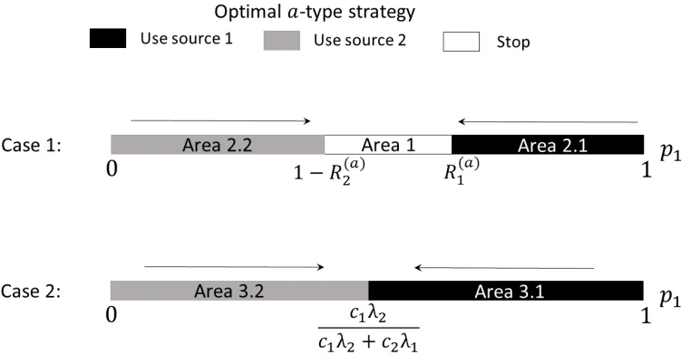
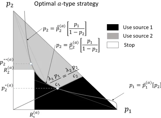
Step 1 Theorem 1 gives the full description of the optimal a-type strategy (see Figures 2.1 and 2.2). It says that for any initial beliefs, the optimal a-type strategy has one of the following forms:

• use source 1 until either the state 1 is revealed or the belief about state 1 drops below the thresholdp1= R

(a)

1 , where

R₁(a) =    

  

c1

λ1(u1[a1]−u1[a]), u1[a1],u1[a], +∞, u1[a1]=u1[a],

(2.6)

• use source 2 until either the state 2 is revealed or p2 = 1− p1 = R

(a)

2 , where

R₂(a) =    

  

c2

λ2(u2[a2]−u2[a]), u2[a2],u2[a], +∞, u2[a2]=u2[a],

(2.7)

• use the source with the highest quality, until the state is revealed by a positive signal; thequalityis defined as the probability of revealing the state to cost ratio:

λ1p1

c1 >

λ2p2

c2 ≡

λ2(1−p1)

c2 ⇒ use source 1,

λ1p1

c1 <

λ2p2

c2 ⇒ use source 2,

λ1p1

c1 =

λ2p2

c2 ⇒ use source 1 and 2 simultaneously,

(2.8)

• do not get any information and choose the default alternativea.

Denote the set of initial beliefs for which not getting any information is optimal as Area 1.

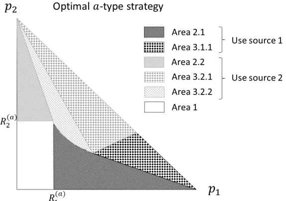
Denote the set of initial beliefs for which “using source 1 until either the state 1 is revealed or the belief about state 1 drops below the threshold p1 = R₁(a)” is the optimal strategy as Area 2.1. Area 2.2 is defined in a similar way. Area 2.1 and Area 2.2 cover the set of initial beliefs for which the optimala-type strategy consists of only the payoff optimal phase.

Denote the set of initial beliefs for which (1) using the source with the highest quality until the state is revealed is the optimal strategy and (2) λ1p1

c1 >

λ2p2

c2 as

(26)

the set of initial beliefs for which the optimala-type strategy consists of only the informatively optimal phase.

The payoff optimal phase of the optimal learning strategy is the phase when the agent will never change the source he is using, no matter what information he receives. In other words, he stays with one source (say, source k) until either the state is revealed to be k or his belief about the state to be k drops to the threshold R(_ka). R(_ka) is interpreted as the ratio of cost over benefit from information source k. Intuitively, the agent stops learning when the marginal cost of learning (ck ·dt) is equal to its marginal benefit, that is, the

probability that the state will be revealed in the next instant of time (pk·λk·dt)

multiplied by the payoff loss from the default alternative if the true state is k (uk[ak] −uk[a]). I call this phase payoff optimal to emphasize that the

optimal choice of the information source depends on the payoff parameters {ui1[ai2]}i1=1,2,3

i2=1,2,3

.

Choosing the source based on comparing λ1p1

c1 and

λ2p2

c2 corresponds to the

informatively optimal phase of the information collection process. I call this phase informatively optimal to emphasize that the optimal choice of the information source does not depend on the payoff parameters. In this benchmark case, when p1+ p2 = 1, the informatively optimal phase always ends with the full revelation of the state. This explains the rule (2.8). Indeed, conditional on the goal of knowing the state with certainty, the agent minimizes the total cost of learning:

C[p1;T]= IE

c1Tτ,1+c2Tτ,2 | p1,p2=1− p1 _,

over the attention allocation planT, whereτis the first time a positive signal is observed. The objective function C[p1;T] does not depend on the payoff parameters, and therefore the optimalT does not either. In the general case, when the probability of the third state is positive, revealing the state with certainty is not feasible when the true state is 3. However, the intuition for the informatively optimal phase is similar. When the agent thinks it is highly likely he is going to know the true state at the end of the information collection process, he chooses the informatively optimal source, that is, the source with the highest quality.

At point p1= _c₁_λc₂1₊λ_c2₂_λ₁, p2 = _c₁_λc₂2₊λ_c1₂_λ₁ both sources are used in proportion to their intensity: dTt,1

dTt,2 =

λ2

(27)

change until the state is revealed. Moreover, at this point the probability of revealing the state at the next instant of time,λ×p×dt, over the cost,c×dt, is the same for both sources: λ1p1

c1 =

λ2p2

c2 .21

,

22

Figures2.1 and2.2 illustrate the optimal a-type strategy by partitioning the intervalp1 ∈ (0,1)into different areas (Area 1, Area 2.1, Area 2.2, Area 3.1, and Area 3.2). Each pointp1corresponds to the agent’s initial belief, and the area number determines what strategy the agent should use.

Another way to describe the optimal a-type strategy is by partitioning the interval p1 ∈ (0,1) into three regions: when to stop learning, when to use source 1, and when to use source 2. This description is equivalent to the one above by the Markovian property of the problem (2.2). At any point in timet, for any initial beliefp0,1, the agent’s optimal behavior depends onp0,1 and all information received so far only through the current beliefpt,1. Thus, partitioning the interval based on the source is equivalent to partitioning the interval based on the whole strategy. Arrows on these figures show how the beliefp1changes in the absence of a positive signal: 0 signals from source 1 decreases p1, while 0 signals from source 2 increases p1. By following the arrows, we can infer the strategy the agent should use. For example, take any p0,1in the source 2 region. If this region is located to the left of the source 1 region,p0,1belongs to Area 3.2. If this region is located to the left of the stop region,p0,1belongs to Area 2.2.

21_{Using both sources in proportion to their intensity leads to the following expected payoff at}

pointp1= _c₁_λc₂1_+cλ2₂_λ₁,p2 =_c₁_λc₂2_+cλ1₂_λ₁: fork=1,2,

(p1u1[a1]+p2u2[a2]) −

c1 λ1 +

c2 λ2

.

This expression is intuitive. Since the agent is going to collect information until the state is revealed, he always chooses the alternative that is the best in this revealed state. Thus, the benefit is his expected utility from the best alternative: p1u1[a1]+p2u2[a2]. The cost of learning from each source

is proportional to the expected time of using this source, which is the expected waiting time for the state to be revealed,_λ1.

22_{Rule (}_2.8_{) can be derived from minimizing}_C_[_p

1;T]overT. Below, I show a sketch of the proof.

LetC[p1]=min

T C[p1;T]. If the agent paysx∈ [0,1]amount of attention to source 1 during the next

instant of time and then implements the optimal allocation rule, his expected cost is equal toc1xdt+

c2(1−x)dt+(1−λ1p1xdt−λ2(1−p1)(1−x)dt)C[p1−λ1p1(1−p1)xdt+λ2p1(1−p1)(1−x)dt]=C[p1]+

c1x

1−λ1p1

c1 (C[p1]+C 0_[_p

1](1−p1))

+c2(1−x)

1−λ2(1−p1)

c2 (C[p1] −C 0_[_p

1]p1) dt ≡

C[p1]+δ[x,p1,C[p1]]dt. If p1 = _c₁_λc₂1_+cλ2₂_λ₁, x = _λ₁λ₊2_λ₂ and C

h

c1λ2

c1λ2+c2λ1

i

= c1

λ1 +

c2

λ2, then

δ[x,p1,C[p1]]=0. Thus, at pointp1 =_c₁_λc₂1_+cλ2₂_λ₁, the attention allocation rulex=_λ₁λ₊2_λ₂ is optimal

since following this rule does indeed giveC h

c1λ2

c1λ2+c2λ1

i

= c1

λ1 +

c2

(28)

Theorem 1 When the probability of the third state is zero, the optimala-type strategy is described as follows. The belief intervalp1 ∈ (0,1)is partitioned into at most five areas (k = 1,2):

Area 1 : for beliefs in this area, stop information collection.

Area 2.k : for beliefs in this area, use source k until pk = R

(a)

k (and then

stop).

Area 3.k : for beliefs in this area, use source k until pk = _cckλ3−k

1λ2+c2λ1 (and

then use both sources in proportion to their intensity, dTt,1

dT_t,2 =

λ2

λ1, until

the state is revealed).

Case 1 If fork = 1,2the following condition holds:

R(_ka) <1, λ3−kR

(a)

3−k

c3−k

≥ λkR

(a)

k

ck

⇒ ∆(_ka) ≤ 0, (2.9)

then

• if1−R₂(a) < p1 < R₁(a), thenp1belongs to Area 1, • if p1> R

(a)

1 , thenp1belongs to Area 2.1, • if p1< 1−R(₂a), thenp1belongs to Area 2.2.

Otherwise, letk ∈ {1,2}be such that:

R(_ka) < 1, λ3−kR

(a)

3−k

c3−k

≥ λkR

(a)

k

ck

, ∆(_ka) > 0. (2.10)

Case 2 If ConditionΠ does not hold, then

• if pk <

c_kλ₃−k

c1λ2+c2λ1, thenp1belongs to Area 3.3-k,

• if pk > _cckλ3−k

1λ2+c2λ1, thenp1belongs to Area 3.k.

Case 3 If ConditionΠ holds, then

• if pk < 1−R

(a)

3−k, thenp1belongs to Area 2.3-k,

• if1−R₃(a₋)_k < pk <min

n ¯

π(a)

k ,R

(a)

k

o

, thenp1belongs to Area 1, • if R(_ka) < pk < π¯

(a)

k , thenp1belongs to Area 2.k,

• ifπ¯(_ka) < pk < _cckλ3−k

1λ2+c2λ1, thenp1belongs to Area 3.3-k,

(29)

[image:29.612.113.494.77.278.2]

Figure 2.1: Illustration for Theorem 1, Case 1 and Case 2. The arrow shows the direction the belief vector is moving while the state is not revealed.

where

∆(_ka) = c3−kλk

ckλ3−k

1 R(₃a₋)_k

−1 !

+log       

ckλ3−k

1−R_k(a)

c3−kλkR(_ka)

      

−1, (2.11)

andConditionΠandπ¯(_ka)are defined in the appendix.

Case 1 covers the set of parameters for which it is never optimal to use both sources simultaneously.23 In Case 2, it is always optimal to learn the state with certainty. Case 3 is a mixture of Case 1 and Case 2.

Condition (2.9) fork = 1,2, guarantees that it is never optimal to implement the rule (2.8).

Given expression (2.11), condition∆(_ka) ≤ 0 has the following interpretation. For each source j, the cost of using the other source (_λc3−j

3−j) is sufficiently

large, as measured by the difference between the benefit of using that source (uj[aj] −uj[a]) and its cost (

cj

λj). In other words, both

c₂

λ₂

u1[a1]−u1[a]−λc1₁ and

c₁

λ₁

u2[a2]−u2[a]−cλ2₂ are large enough to make sure that when the state is likely to be

23_{Condition (}_2.9_{) guarantees that 1}₋_R(a)

2 ≤R

(a)

(30)

Figure 2.2: Illustration for Theorem1, Case 3. The arrow shows the direction the belief vector is moving while the state is not revealed.

j (i.e., when pj ≥ R

(a)

j ), to decide betweena andaj it is optimal to use only

source j, which provides “direct” information about the state being j or not, rather than rely on “indirect” information from source 3− j.

Expression (2.11) can be rewritten as

∆(_ka) =

V(a)[p1]

Area 3.k

−V(a)[p1]

Area 2.k

ck

λk(1−pk)

,

where V(a)[p1]

AreaX

is the expected payoff from the strategy described in

(31)

2.k.24,25

At point ¯π(_ka), the agent is indifferent between using at most one source in his learning strategy and applying the Area 3.3-k strategy. Condition Π

guarantees that such a point exists.26

Generally speaking, the optimal a-type strategy is unique. It means for all beliefs (except the set of measure zero) and for all other parameters’ values (except the set of measure zero), the optimal action (what source to choose and when to stop) is unique. Indeed, the expected payoff from different strategies is almost never the same. The nonuniqueness can happen only at the indifference points. For some parameters’ values, such indifference points might form the whole interval. For example, when ¯π(_ka) =1−R(₃a₋)_k, the whole intervalpk ≥ 1−R

(a)

3−k is such that the agent is indifferent between Area 2.3-k

and Area 3.3-k strategies. However, the set of such parameters’ values has measure zero.

Step 2 . Given initial beliefp1, the optimal strategy is the optimala-type strategy, wherea ∈ AmaximizesV(a)[p1].

Though sufficient for computing the optimal strategy, this description is not very illustrative. Another way to describe the optimal strategy is as follows.

Denote byVk[p1], k = 1,2, the expected payoff from the optimal strategy if only source k is available. Denote this strategy as k-strategy. This strategy

24_{Comparing these two strategies, one must also take into account their feasibility: Strategy}

in Area 2.k only makes sense if pk ≥ R

(a)

k , while strategy in Area 3.k is feasible if and only if

pk ≥ _c₁ck_λ₂λ_+c3−k₂_λ₁. However, condition∆

(a)

k >0 does not depend on beliefs. Thus, if∆

(a)

k >0, then

it is optimal to use strategy from Area 3.k for all pk ≥max

n

R_k(a),1−R₃(a₋)_k, ckλ3−k c1λ2+c2λ1

o

: pk ≥ R

(a)

k

guarantees that Area 2.k strategy is feasible and is better than no learning, inequalitypk ≥1−R

(a)

3−k

excludes the Area 2.3-k strategy. By the Markovian property, it is optimal to use strategy from Area 3.k for allpk ≥ _c₁ck_λ₂λ_+c3−k₂_λ₁. This reflects in Case 2 and 3, where Area 3.k covers the whole interval

pk ∈

1, ckλ3−k c1λ2+c2λ1

.

25_{Condition (}_2.9_{) is a more subtle than just}_∆(a)

k ≤0. ConditionR

(a)

k <1 is necessary for Area

2.k strategy to be feasible. Moreover, forR(_ka)≥1,∆(a)

k is undefined. SupposeR

(a)

k <1. Condition

(2.9) per se does not rule out the case when λ3−kR

(a)

3−k c3−k <

λkR(a)_k ck and∆

(a)

k >0. However, condition

(2.9) fork =1,2 together do imply∆(a)

i ≤0 whenever R

(a)

i < 1 fori =1,2 (see Remark2in the

appendix for the proof).

26_{Note that point ¯}_π(a)

k must always be above 1−R

(a)

3−k. Indeed, by the Markovian property, for

pk ≤1−R

(a)

3−k, Area 2.3-k strategy is better than Area 3.3-k strategy if and only if it is better at point

pk =1−R

(a)

(32)

consists of the payoff optimal phase. 27

Denote byV3[p1]the expected payoff from the following strategy (denote this strategy as∞-strategy):28

• if p1> _c₁_λc₂1₊λ_c2₂_λ₁, use source 1,

• if p1< _c₁_λc₂1₊λ_c2₂_λ₁, use source 2,

• at point p1= c1λ2

c1λ2+c2λ1, use both sources in proportion to their intensity.

This strategy consists of the informatively optimal phase.

IfVk[p1] ≥ max{V3−k[p1],V3[p1]}for somek =1,2, then the optimal strategy is the k-strategy; ifV3[p1] ≥ max{V1[p1],V2[p1]}, then the optimal strategy is the∞-strategy. This description is more intuitive since it does not involve maximization over a ∈ A but rather emphasizes the strategic tradeoff the agent faces. He compares the costs and benefits of information to decide whether it is optimal to learn the state with certainty (∞-strategy) or if he should “give up” at some point if he does not observe a positive signal for a sufficiently long time (1-strategy or 2-strategy).

Figure2.3 shows two examples of the optimal strategy defined as a partition of the belief interval into three regions (use source 1, use source 2, stop the information collection process). These examples illustrate two general features of the optimal strategy. First, if the agent is ever going to use both sources, he does it at point p1 = c1λc21+λc22λ1. Thus, if either 1-strategy or

2-strategy is better than ∞-strategy at this point, there is no initial belief such

27_{See Section}_2.4.2_{for the explicit form of}_V k[p1]. 28_If_p

k ≥ _c₁ck_λ₂λ_+c3−k₂_λ₁, this payoff is

V3[p1]=(p1u1[a1]+p2u2[a2]) −

p3−k+

ckλ3−k

c1λ2+c2λ1

c1 λ1 +

c2 λ2

−ckp3−k

λk

log

pk

p3−k

c3−kλk

ckλ3−k

.

Part p1u1[a1]+p2u2[a2]accounts for the utility the agent gets from the chosen alternative at the

end of the information collection process. The rest is equal to the expected cost of collecting information. Whenpk = _c₁ck_λ₂λ_+c3−k₂_λ₁, this cost is equal to_λc1₁ +_λc₂2. Whenpk > _c₁ck_λ₂λ_+c3−k₂_λ₁, the middle

term,p3−k+_c₁ck_λ₂λ_+c3−k₂_λ₁ _λc1₁ +_λc2₂

, is less thanc1

λ1+

c2

λ2, while the last term,

ckp3−k

λk log

h _pk

p3−k c3−kλk ckλ3−k

i ,

is positive. Moreover, when pk > _c₁ck_λ₂λ_+c3−k₂_λ₁, the expected cost decreases in pk, which means

p3−k +_c₁ck_λ₂λ_+c3−k₂_λ₁ c_λ1₁ +c_λ2₂

+ckp3−k

λk log

h _pk

p3−k c3−kλk ckλ3−k

i

< c1

λ1 +

c2

λ2.

Intuitively, this follows from the optimality of the strategy. The strategy to use both sources until the state is revealed is always feasible, which means the expected payoff(p1u1[a1]+p2u2[a2])−

c1

λ1 +

c2

λ2

(33)

Figure 2.3: Illustration of the optimal strategy when the probability of state 3 is zero. The arrow shows the direction the belief vector is moving while the state is not revealed.

that∞-strategy is optimal.29 Second, if the agent chooses the k-strategy and does not “give up” immediately, the default alternative is eithera3−k or a3.

Indeed, the information benefit of using source k is proportional to the cost of mistake,uk[ak] −uk[a]. If the default alternativeaisak, then this cost is 29_{Formally, when the probability of the third state is zero and}

R(a2)

1 <1, R

(a1)

2 <1, R

(a3)

k <1, ∆

(a2)

1 >0, ∆

(a1)

2 >0, ∆

(a3)

k >0, wherek∈

(

{1,2}: λkR

(a3)

k

ck

≤ λ3−kR (a3)

3−k

c3−k

)

,

(2.12) then there exist two thresholds, 0<p

1 < c1λ2

c1λ2+c2λ1 <p¯1 <1 such that it is optimal to implement the ∞-strategy for allp1 ∈

h p

1,p¯1

i

; for other beliefs, it is optimal to implement thek-strategy, where k ∈ {1,2}is such thatVk[p1] ≥V3−k[p1]. If condition (2.12) does not hold andk ∈ {1,2}is such

thatVk[p1] ≥V3−k[p1], then the optimal strategy is thek-strategy.

Condition (2.12) can be rewritten as follows:

1

R(a2)

1

> c2λ1

c1λ2

e1+

c2λ1

c1λ2 ₊₁_, 1

R(a1)

2

> c1λ2

c2λ1

e1+

c1λ2

c2λ1 ₊₁_,

λkR

(a3)

k

ck

≤ λ3−kR (a3)

3−k

c3−k

⇒ 1

R(a3)

k

> c3−kλk

ckλ3−k

e

1−c3−kλk ckλ3−k

1

R₃(a_−k3)

−1

!

+1. (2.13)

(2.13) means the cost of mistake — that is,u1[a1] −u1[a2],u2[a2] −u2[a1], anduk[ak] −uk[a3]for

(34)

zero and therefore, source k offers no benefit. This feature explains why it is sometimes optimal to use the source that has low ex ante probability to reveal the state (see “use source 1” region near p1 = 0 and “use source 2” region nearp1= 1).

2.4.2 Three States, One Source

In this section, I present the optimal strategy when there is only one information source available to the agent (suppose it is source 1):

sup

(a,τ)

IEuj[a] −c1τ | p1,p2 _.

(2.14)

This is a standard optimal stopping problem (Wald and Wolfowitz (1948), Dynkin (1963), Dragalin, Tartakovsky, and Veeravalli (1999), Dragalin, Tartakovsky, and Veeravalli (2000), Shiryaev (2007)). Usually, it is formulated with two states and two alternatives. Technically, the generalization to three states and three alternatives is straightforward. However, it provides new insight to the general model I present in Section2.5.

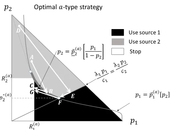
The Markovian property of the problem — at any point in time t, for any initial beliefs (p0,1,p0,2), the agent’s optimal behavior depends on initial beliefs and all information received so far only through the current beliefs(pt,1,pt,2)— allows for representing the optimal strategy as a partition of the belief triangle

{(p1,p2) ∈ [0,1]2: p1+ p2≤ 1}

into two regions: “use source 1” and “stop.” The “use source 1” region is the set of beliefs (p1,p2)such that if the agent’s current beliefs fall into this set, he pays his full attention to source 1. The “stop” region corresponds to the set of current beliefs where it is optimal to stop collecting information and choose an alternative.

By definition, the information source 1 separates state 1 from the other two states, meaning the information from this source cannot affect the agent’s belief about the relative probabilities of states 2 and 3. Formally, the ratio pt,2

1−pt,1 stays constant

throughout the learning process. Moreover, unless the state 1 is revealed, the belief about state 1 decreases during the learning process. Graphically, source 1 moves the belief vector along the line that holds the ratio p2

1−p1 constant, away from the corner

p1=1 (see Figure2.4).

(35)

and the default alternative. By the Markovian property, defining a “give up” time is equivalent to defining the belief threshold p1= p

1. Once the agent’s belief reaches this threshold, he stops the information collection.

Lemma 1 gives the explicit form of the expected payoff from the strategy with a given threshold p1= p

1and the default alternativea∈ A.

Lemma 1 Given the initial beliefs (p1,p2), any threshold p

1 ∈ (0,p1] and any default alternativea ∈ A, the expected payoff from using source 1 until either state 1 is revealed (anda1is chosen) or the belief reaches the threshold p1 = p

1 (anda

is chosen), whichever happens first, is the following:30

V₁(a) h

p1,p2;p 1

i

= 1−p1 1−p

1

u1[a]p 1+

u2[a]

p2

1− p1 +u3[a]

1− p2

1−p1 (1−p1)

+ p1−p1 1−p

1

(1−p1)log        p1

1−p 1

p

1(1−p1)       

+ p1− p1 1−p

1 ª ® ® ¬ . (2.15)

Expression (2.15) has three terms. The first term, 1−p1

1−p 1

u1[a]p

1+

u2[a] p2 1−p1 +

u3[a]

1− p2

1−p1

(1−p 1)

is the probability that state 1 is not revealed by the end of the information collection process multiplied by the expected utility from choosing the default alternative. The second term, p1−p1

1−p

1

u1[a1], is the probability that state 1 is revealed before the “give up” time multiplied by the payoff from choosing alternative a1at state 1. The last term is the expected total cost of using source 1.

As with the two states, two sources setup in Section 2.4.1, I split the solution into two steps. First, I find the optimal a-type strategy by maximizing (2.15) over p

1. Then, given the optimal threshold p

1, I maximize (2.15) over all possible default alternativesa ∈ A.

30_{The expected payoff from the symmetric contingency plan with source 2 instead of source 1 is}

V₂(a) h

p1,p2;p 2

i

= 1−p2

1−p

2

u2[a]p

2+

u1[a]

p1

1−p2

+u3[a]

1− p1

1−p2

(1−p

2)

+p2−p2

1−p

2

u2[a2] −

c2 λ2 © «

(1−p2)log

       p2 1−p

2

p

2(1−p2)

      

+ p2−p2

1−p

2 ª ® ® ¬ .

I use the expressionV_k(a)hp1,p2;p k

i

(36)

Figure 2.4: Illustration for Theorem 2. The arrow shows the direction the belief vector is moving while the state is not revealed.

Theorem2 describes the optimal a-type strategy. It states that (2.15) achieves its maximum atp

1 =min{p1,R

(a)

1 }, whereR

(a)

1 is defined by (2.6):

Theorem 2 When only source 1 is available, for any initial beliefs, the optimal

a-type strategy,a ∈ A, is to use source 1 if and only if the agent is uncertain about the state and the current belief about the probability that the true state is 1 is no less thanR₁(a).

Theorem2shows that the threshold rule p1= R₁(a) derived in Theorem1extends to a general case when p1+p2 ≤ 1.

Figure2.5shows how a very simple form of the optimala-type strategy might lead to a complex description of the optimal strategy on the belief triangle. This complexity is the main reason to split the solution into two steps and derive the optimala-type strategy first. Figure 2.5 is derived by comparing the expected payoff from the optimala1-type,a2-type, anda3-type strategies, for each point in the belief triangle. It illustrates the optimal strategy by partitioning the belief triangle into two regions: where information collection is optimal and where it is not. For any beliefs(p1,p2) where information collection is optimal, the default alternative is determined by following the belief trajectory along the line with constant p2

1−p1 ratio away from