The effect of spatial averaging on dB/dt exposure values for implanted medical devices

(1)

Scholarship@Western

Electronic Thesis and Dissertation Repository

8-28-2019 2:00 PM

The effect of spatial averaging on dB/dt exposure values for

implanted medical devices

Christopher AP Brown

The University of Western Ontario

Supervisor Chronik, Blaine A.

The University of Western Ontario Graduate Program in Physics

A thesis submitted in partial fulfillment of the requirements for the degree in Master of Science © Christopher AP Brown 2019

Follow this and additional works at: https://ir.lib.uwo.ca/etd Part of the Physics Commons

Recommended Citation Recommended Citation

Brown, Christopher AP, "The effect of spatial averaging on dB/dt exposure values for implanted medical devices" (2019). Electronic Thesis and Dissertation Repository. 6512.

https://ir.lib.uwo.ca/etd/6512

This Dissertation/Thesis is brought to you for free and open access by Scholarship@Western. It has been accepted for inclusion in Electronic Thesis and Dissertation Repository by an authorized administrator of

(2)

Abstract

Magnetic resonance imaging (MRI) is a medical imaging modality that has seen

continuous growth in the decades since its introduction. In conjunction with this

increase in the use of MRI, there has also been a growth in the number of patients

having implanted medical devices, such as pacemakers. These devices can have

undesirable interactions with the MR system. The safety of these interactions must

be guaranteed while ensuring that safety limits are not so conservative that they

would preclude too many patients from benefiting from MRI. One factor that could

make limits less restrictive is spatial averaging of the fields in MRI.

The objective of this investigation was to determine the effect that spatial

averaging would have on the predicted time-varying magnetic field (dB/dt) values

within realistic MRI gradient systems. ISO/TS 10974:2018(E) contains simulated

data describing the peak dB/dt values that active implantable medical devices

(AIMDs) could be exposed to when within varying volumes within the bore of the

MRI scanner to account for the device location dependence of the dB/dt. For

devices with realistic spatial extent (e.g. a 5 cm diameter component), the dB/dt

relevant for testing would need to include information about the spatial average of

the dB/dt over the device.

This investigation involved the development and validation of a numerical

software system to simulate the fields produced by arbitrary gradient coil designs

at any point within the gradient and for any device geometry placed within that

(3)

measurements, and it was shown that the mean and peak dB/dt values differ

between 2 and 17%. The difference between the peak and mean values increases

monotonically with the distance from the central axis of the gradient coils.

Keywords

(4)

Summary for lay audience

Magnetic resonance imaging (MRI) is a medical imaging modality that is becoming

more and more common. For healthy patients, it is known to be a very safe

imagining modality, as it does not make use of any of the damaging radiation

present in other imaging techniques like x-rays. However, when patients have an

implanted medical device, like a pacemaker, as part of their treatment, this can lead

to undesirable interactions with the MRI scanner. Patients with health

complications benefiting from these medical devices are often those who would

most benefit from MRI, so there is a need to guarantee that patient safety is assured

while still allowing as many people as possible to be scanned.

One of the most important parts of every MRI system is the gradient coil.

This coil produces a time varying magnetic field, called a dB/dt. In order to take

full advantage of the power of MRI, it is desirable for this dB/dt value to be as large

as safely possible. However, the larger the dB/dt, the greater the interaction with a

medical device.

Current safety standards only refer to the peak dB/dt values that devices

could be exposed to within the bore of the MRI scanner. But for devices realistic

devices, the dB/dt relevant for testing would need to include the spatial average of

the dB/dt over the device.

This investigation examined the effect that this spatial averaging would

have on dB/dt exposure to ensure that safety limits are not too conservative, so that

(5)

Co-Authorship Statement

The work presented in chapter 2 relies on data previously collected by Christine

Tarapacki using a probe designed by Ryan Chaddock controlled using a robotic

measurement system designed by Jack Hendriks. The dB/dt coil was designed by

Daniel Martire and built by the Chronik research group.

The work presented in chapter 3 has been submitted as an abstract to the

International Society of Magnetic Resonance in Medicine (ISMRM). This work

also seeks to be published. Brown lead the research and produced all scripts and

simulations and performed all analysis. Drs. Handler and Harris wrote the code to

design the gradient coils used in the simulations. Dr. Chronik funded and

(6)

Acknowledgements

This thesis could not have been completed without the support and generosity of

all those who have helped me not only over the past two years, but throughout my

entire education.

First and foremost, thank you to my supervisor, Dr. Blaine Chronik, not

only for the knowledge he has shared, but the invaluable opportunities provided by

working as a member of his research group for the past six years.

I would also like to especially thank Dr. William Handler, whose

knowledge, wisdom and expertise are more than made up for by his sense of

humour.

Thank you to the other members of the research group during my time here,

Dr. Geron Bindseil, Colin McCurdy, Justin Peterson, Christine Wawrzyn,

Krzysztof Wawrzyn, Dr. Ali Attaran, Dr. Saghar Batebi and Dr. John Drozd, for

their help and advice.

The apparatuses used in this research could never have been brought to life

without the expert technical knowledge of Frank Van Sas, Brian Dalrymple, Ryan

Chaddock, Jack Hendriks and Dereck Gignac.

Thank you to my fellow graduate students, past and present, Amgad Louka,

Eric Lessard, Kieffer Davieau, Arjama Halder, Xiao Fan Ding, Diego Martinez,

John Adams, Daniel Martire and Spencer Parent, with whom it has been a privilege

(7)

Thank you and much love to my parents and my sister Julia, who have been

there for me every step of the way with love and support.

I would also like to acknowledge the help of my advisory committee, Dr.

Lyudmila Goncharova and Dr. Giovanni Fanchini, as well as all the members of

my examination committee, Dr. Corey Baron, Dr. Alexei Ouriadov and Dr. Olga

Trichtchenko.

This work has been supported by the following sources of funding: NSERC,

(8)

List of Tables

Table 3.2-1: The spatially averaged dB/dt compared to the peaks at three different

step sizes in z for the 60 cm inner diameter, 160 cm length, 45 cm imaging region

coils, at a 25 cm compliance radius. The angular resolution was at 10 degrees. A z

step of 10 cm was decided upon for the simulations of the final family of coils as a

trade off to still have a reasonable runtime.

Table 3.2-2: The spatially averaged dB/dt compared to the peaks at three different

step sizes in the angular spacing for the 60 cm inner diameter, 160 cm length, 45

cm imaging region coils, at a 25 cm compliance radius. A z step of 10 degrees was

decided upon for the simulations of the final family of coils as a trade off to still

have a reasonable runtime.

Table 3.2-3: The percent difference between the spatially averaged dB/dt and the

peaks by component and magnitude of the dB/dt vector. Three different step sizes

in z are shown for the 60 cm inner diameter, 160 cm length, 45 cm imaging region

coils, at a 25 cm compliance radius.

Table 3.3-1: The maximum dB/dt by compliance radius for the family of coils at

a slew rate of 200 T/m/s. Note that the dB/dt component labels shown above do

not correspond to gradient axes but indicate the components of the dB/dt vector.

The right-most three columns list the peak (no spatial averaging values) obtained

for the individual dB/dt components. Note also that the magnitude column does

not correspond to the quadrature sum of the peak x-, y-, z-components of the

(11)

List of Figures

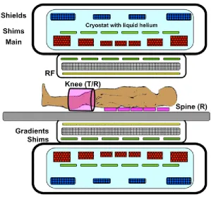
Figure 1.2-1: A cross-section of a modern, cylindrical bore superconducting MRI

system. The three main components are the main magnet, shown in the outer layer,

the gradient coil, shown in the second layer, and the RF coil, shown in yellow. Each

of these three main components will be discussed in this section [16].

Figure 1.2-2: A sample 𝑘-space and its equivalent image [17]. Each pixel in the

𝑘-space represents a spatial frequency in the equivalent MR image, with the

intensity of that pixel representing the relative importance of that spatial frequency.

Note that this image only shows the real valued data. In practice, each point in 𝑘

-space is a complex number with both magnitude and phase. Points closer to the

center of 𝑘-space correspond to lower spatial frequencies, meaning broader, more

general shapes, while points closer to edge represent high frequency, small scale

details. The strength of the gradient influences the resolution of the images for a

given imaging time, since it determines how far out in k-space the scanner can go,

which gives higher and higher frequency information. Because of this, high

gradient strength is desirable. This figure also shows that the image on the left and

its 𝑘-space are equivalent in the information that they hold. One can be completed

reconstructed from the other.

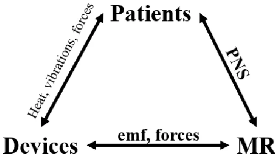
Figure 1.3-1: The three different broad categories of interactions that occur in MRI:

patient/device interactions, patient/MR scanner interactions, and device/MR

(12)

to consider not alone interactions between the patient and the scanner, but also

between devices, the scanner and the patient.

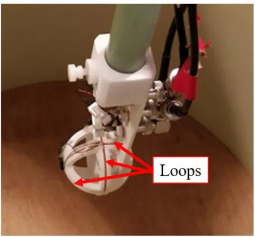
Figure 2.2-1: The probe used to collect dB/dt measurements. The probe had 3-axes

corresponding to the Cartesian axes, with the three loops consisting of 10 loops of

copper wire each with a 5.0 cm loop diameter, shown by the arrows. The set of

loops hidden by the lip of the white mound corresponds to the z axis in this case,

since it has its normal oriented along the bore of the coil.

Figure 2.2-2: The experimental setup. In the foreground is the robotic system used

to collect the field data over the volume of the dB/dt coil, the cylindrical system in

the midground. The grey regions contain the wire windings of the coil.

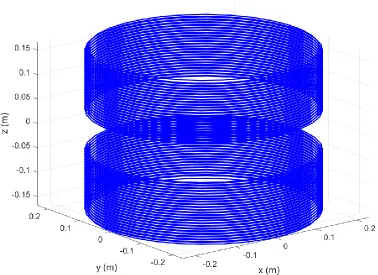
Figure 2.2-3: The wire pattern on the dB/dt coil. The coil is a large bore split

solenoid. Visible are the two layers of wire windings, with the inner layer having

24 windings, and the outer layer having 23.

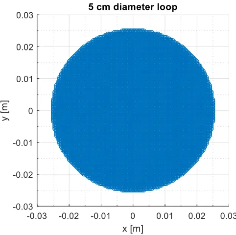
Figure 2.2-4: The simulated loop of the probe. It had a 5.0 cm diameter and a

surface discretization of 0.5 mm, resulting it of 7860 points on the device.

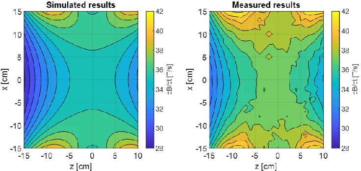
Figure 2.3-1: The spatial distribution of the simulated dB/dt within the bore for the

plane y = 0 cm. Note that the z-direction is along the bore of the coil.

Figure 2.3-2: The spatial distribution of the measured dB/dt within the bore of coil

for the plane y = 0 cm. Note that the z-direction is along the bore of the coil.

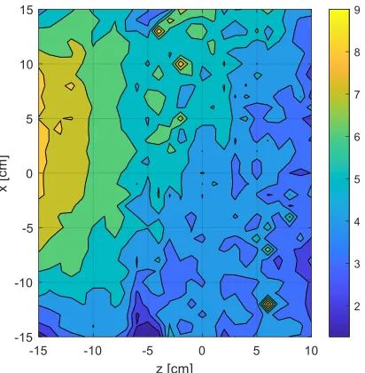
Figure 2.3-3: The spatial distribution of percent differences between the measured

and simulated values within the bore of coil for the plane y = 0 cm. Note that the z

(13)

the measurements is a result of the limitations of the reach of the positioning

system.

Figure 2.3-4: The spatial distribution of percent differences between the measured

and simulated values within the bore of coil for the plane z = -10 cm. Note that the

z-direction is along the bore of the coil.

Figure 2.3-5: A histogram of the percent differences between the measured values

and the simulated data. The distribution of the errors is influenced by the precision

limitations of the oscilloscope used to major the induced voltages, which in turn

determine the measured dB/dt values.

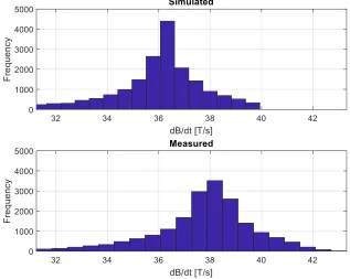
Figure 2.3-6: Histograms of the dB/dt distributions for both the simulated (top) and

measured (bottom) values. Note the systematic difference between the two. The

simulation consistently underpredicts the measurements.

Figure 2.3-7: A comparison between the predicted field values along y, and the

measured values along x. The ideal case of perfect equality is shown overlaid in

red.

Figure 3.2-1: The 5.0 cm diameter spherical volume used as the ‘device’ in these

simulations, with the points on the surface in red and the points in interior in blue.

The blue points are discretized in a grid with a 5 mm separation between points

along each axis. The red points are equal in number to the blue points but equally

(14)

Figure 3.2-2: The calculation grid for the 20 cm compliance radius case. Note that

the radius is slightly less than 20 cm at 17.5 cm so that the 5.0 cm diameter device

volume with its center at any point on this grid will extend to 20 cm at most.

Figure 3.2-3: The 5.0 cm diameter spherical device in red at a single point of

the surface of one compliance radius. The compliance radius it located within a

single example gradient, the 60 cm inner diameter, 140 cm length, and 35 cm

imaging region, for the z gradient, shown in black. The blue points, extending

from -1 m to 1 m, represent each position at which the device is positioned and

simulated for each coil combination.

Figure 3.3-1: Histogram of the dB/dt (magnitude) at all 777 points within one

example coil: x gradient of 60 cm diameter, 160 cm length, 45 cm imaging region

coil at a 25 cm compliance radius. Values are given as dB/dt per unit slew rate of

the gradient axes. For a 200 T/m/s scanner system, the values above need to be

multiplied by 200.

Figure 3.3-2: Histogram of all the data across all the coils (and all compliance

volumes) with the 95th and 99th percentiles shown (0.352 T/s per slew rate and

0.443 T/s per slew rate). For a 200 T/m/s scanner system, the values above need to

be multiplied by 200.

Figure 3.3-3: The peak spatially averaged dB/dt value across each coil in the

simulation space at 4 different compliance radii. Values are given as dB/dt per unit

slew rate of the gradient axes. For a 200 T/m/s scanner system, the values above

(15)

List of Abbreviations and Symbols

AIMD Active implantable medical device

ASTM American Society for Testing and Materials

B Magnetic flux density

CT Computed tomography

dB/dt Time-varying in magnetic field

FDA Food and Drug Administration

ISO International Organization for Standardization

MRI Magnetic resonance imaging

NMR Nuclear magnetic resonance

PET Positron emission tomography

PNS Peripheral nerve stimulation

RF Radiofrequency

TE Echo time

TR Repetition time

(16)

Chapter 1: Introduction

This chapter introduces Magnetic Resonance Imaging (MRI) as an imaging

modality and explains how some of the components within the scanner required to

produce images can interact with medical devices. These interactions must all be

considered when trying to classify the safety of devices for use in MRI, which

determines whether patients who have active implantable medical devices

(AIMDs), for example, can undergo an MR imaging procedure. A brief overview

of the entire MRI assembly is given. The electromagnetic interactions that these

devices experience with the MR system will be reviewed, focusing mainly on the

interactions with the subsystem called the gradient coils. The chapter concludes

with a description of the research objectives of this thesis.

1.1 Motivation

1.1.1 Why MRI?

Magnetic resonance imaging, or MRI, is a medical imaging modality. It is desirable

because it provides excellent soft tissue contrast at high resolution without the use

of ionizing radiation, or invasive intervention like biopsy [3]. In fact, MRI scans

can even be used to identify tumors or bone fractures that are too small for other

types of imaging like x-ray imaging [4].

Ionizing radiation includes any particle incident on the patient of sufficient

(17)

irreparable damage at higher doses. For example, computed tomography (CT),

another widespread medical imaging modality, makes use of x-rays, which are high

energy photons. In positron emission tomography (PET), gamma rays, which are

photons of even greater energy than x-rays, are emitted, among other particles. In

such imagining modalities, patient exposure to radiation must be carefully

monitored to ensure safety [5].

MRI does not require any such exposure limitations. If established safety

standards are followed, a patient could be scanned every day with no adverse effects

on their health. These safety standards, and the associated safety concerns, have

inspired the topic of investigation of this thesis, and will be discussed in more detail

in later sections of this chapter.

Because of the advantages of MRI, millions of MR imaging exams are now

conducted globally every year [32]. In Canada alone, around 1 million exams were

performed in 2007. That number increased to 1.7 million MR exams conducted in

2012 [6], and increased further in 2017, with an estimated 1.86 million MRI

examinations performed [7].

1.1.2 Why is considering medical devices important?

As standards of health care improve and new forms of treatment are developed,

there is not only an increase in the number of MRI scans performed, but it is

increasingly common for patients to have implanted medical devices as a part their

(18)

cardiac implants (i.e. pacemakers and implantable cardioverter defibrillators).

There were over 370,000 implants of cardiac pacemakers in the United States in

2003 [8], and over 135,000 implants of cardiac systems in Canada in 2006 [10, 11],

and this only for one of the many categories of device (see section 1.3.1). The

congruent growth in MRI availability and device use makes device safety within

MR an important problem.

As previously mentioned, a healthy volunteer could be scanned every day

with no adverse effects. However, because of their different material composition,

medical devices, they will behave differently than biological tissues when within

the complex electromagnetic environment of the scanner. These differences in

behavior must be characterized prior to any imaging procedure. Devices can

experience strong forces, heating, vibration, and operational failure. In addition to

direct patient safety concerns, the presence of devices can affect image quality,

reducing diagnostic effectiveness [13]. Later sections in 1.3.3 will go into these

hazards in more detail.

Since the individuals who get medical implants already have compromised

health, they are often those who would most benefit from the diagnostic capabilities

of MRI to monitor their health and to track the effectiveness of treatment. Because

of this, it is essential that MRI is safe and accessible for as many patients as

possible. For patients with the aforementioned cardiac implants, 50 to 75% are

expected to be referred to an MRI over the lifetime of the device in order to track

the current status of their health. However, in the United States alone, it is estimated

(19)

systems in 2004 [8]. Understanding these hazards is thus of vital importance to

ensure patient safety during scanning procedures, while also ensuring that safety

standards are not so restrictive that patients who could still benefit from an MRI are

being denied. Labeling provided by device manufacturers must be accurate so that

medical professionals can make an appropriate informed decision when

determining whether a patient may undergo an MR procedure.

The standards governing the safety of medical devices are decided upon by

the regulatory bodies ASTM (American Society for Testing and Materials) and ISO

(International Organization for Standardization) [20]. Under these organizations,

committees are formed to investigate interactions that devices can experience and

to quantify their impact on patient health. As new investigations are performed and

interactions are better understood, these safety standards are subject to change, with

revisions published every several years.

There is already such a wide array of devices (see section 1.3.1) and MRI

systems that there are far too many scenarios to physically test [22], and there are

new devices are also being developed constantly. Regulatory labelling often makes

use of physically validated computer simulations to model devices and MRI

systems. This aids in identifying a manageable number of worst-case scenarios

under which devices should be physically tested.

However, when considering safety scenarios, there must necessarily be a

balancing act between ensuring patient safety with respect to medical devices in

MRI and allowing as many patients as possible to benefit from MRI. If only

(20)

restrictive. This reduction in accessibility reduces the benefit of MRI as a diagnostic

tool.

This thesis seeks to develop a computer simulation for modeling the

magnetic environment produced by one of the MRI subsystems, the gradient coils,

across any arbitrary system design. The simulation tool is then used to evaluate the

effect that spatial averaging will have on the time-varying field exposure values

when compared to the peak exposure. It is predicted that the decrease in exposure

between the two will ensure that safety standards are not too conservative, and that

regulatory bodies have as much information as possible when deciding about

(21)

1.2 MRI systems

The research included in this thesis does not pertain to any new developments in

imaging or image processing. It is dedicated to ensuring that new advances in

imaging can be performed safely. To that end, discussion of MRI is limited to a

description of the magnetic environment necessary to image, and how this

environment can lead to safety concerns. For a more advanced discussion of the

process of image acquisition in MRI, refer to Magnetic resonance imaging:

Physical principles and sequence design, [1] in addition to a more detailed

description of the topics covered in this section.

Modern MRI systems are very complex and require many independent

subcomponents in order to create an image. A typical MR scanner will contain

several magnets: the main magnet, the radiofrequency (RF) coils, and the gradient

coils, each of which will be outlined in this section. Each of the different fields in

MRI interact with patients and implanted devices differently and have their own

(22)

Figure 1.2-1: A cross-section of a modern, cylindrical bore superconducting MRI system. The three main components are the main magnet, shown in the outer layer, the gradient coil, shown in the second layer, and the RF coil, shown in yellow. Each of these three main components will be discussed in this section [16].

1.2.1 The main magnet

Magnetic resonance imaging operates on the principle of nuclear magnetic

resonance (NMR). Imaging via NMR is possible because of the presence of

unpaired nucleons in the nuclei of atoms inside the body, producing a net spin and

magnetic moment in that nucleus. Most clinical MRI relies on the resonance of

protons found in water molecules throughout the body. Because of the abundance

(23)

to produce the best signal. Note that it is possible to obtain information similarly

using any atom with a net magnetic moment, such as carbon-13 or sodium-23.

When discussing MRI, it is common to consider the behaviour of nuclei as

described by classical physics. On its own, a single nucleus will not produce a very

strong signal. In the classical analogy, the magnetic moments of many atoms align

with the external field, producing a net magnetization within a sample. In MRI, this

initial external field is produced by the main magnet. It is referred to as 𝐵0, where

𝐵 is the standard variable in electromagnetism used to represent the magnetic flux

density, measured in tesla (T), and the subscript is used to emphasize its static

nature within the MR scanner. Clinical MR systems vary in main magnetic field

strength from 0.2 T to 10.5 T systems.

Nuclei that possess net magnetic moments will produce an electromagnetic

signal when perturbed by a specifically designed magnetic field oscillating at an

intrinsic resonant frequency. The rate of precession (𝜔₀) of the magnetization about

the field in MRI is called the Larmor frequency, and it depends on the field strength

(𝐵0) and a nuclei dependent proportionality factor called the gyromagnetic ratio

(𝛾). In the presence of other fields, the 𝐵0 term is replaced by the net magnetic field

that the nuclei experience.

𝜔₀ = 𝛾𝐵₀ (1.2-1)

For protons, which are found unpaired in every water molecule, the

gyromagnetic ratio is 42.577 MHz/T. This means that in a 1 T field, they would

(24)

fields needed to produce this resonance are radiofrequency (RF) fields. The coils

used to produce these fields are discussed in the next section. The gyromagnetic

ratio of these protons is also higher than that of other nuclei that can be used in

imaging, like carbon-13 and sodium-23. This produces a stronger signal in the

receiver and makes it easier to spatially distinguish information.

At higher 𝐵₀ fields, in addition to the increased resonant frequency, a

greater magnetization linearly proportional to the field is produced. In a

paramagnetic material like water, this relationship is described by Curie’s law.

𝑀⃑⃑ = 𝐶𝐵⃑ 𝑇

(1.2-2)

The magnetization (𝑀) is described in amperes per meter and is dependent on a

material specific Curie constant (𝐶) in kelvin amperes per tesla meter, the magnetic

flux density (𝐵) in tesla, and the temperature (𝑇) in kelvin. [1] This greater

magnetization produces a stronger signal, increasing the signal-to-noise ratio,

making it easier to acquire better quality images. However, higher 𝐵₀ field strength

magnet systems produce greater heating, have a greater sensitivity to field

inhomogeneities, and cost much more.

In order to produce such high fields with a high magnetic field homogeneity

over a large volume, the main magnets in modern MRI scanners have evolved to

be cylindrical in shape, consisting of loops of superconducting wire wound around

the bore. The main windings of this magnet are shown as the red bundles in the

outer layer of figure 1.2-1.When a constant current is passed through the wires, a

(25)

𝐵⃑ (𝑟 ) = 𝜇0 4𝜋∫

𝐼𝑑𝑙⃑⃑⃑ × 𝑟̂′

|𝑟_{⃑⃑⃑ |}′ 2 𝐶

(1.2-3)

Here, 𝐵⃑ is again the magnetic flux density described in tesla, 𝜇₀ is the vacuum

permeability in henries per meter, I is the current in amperes, 𝑑𝑙⃑⃑⃑ is an infinitesimal

length of the wire conductor in meters, and 𝑟_⃑⃑⃑′_{is the vector representing the distance}

between the conductor element and the point at which the 𝐵⃑ field is calculated.

The main magnet is designed such that the 𝐵₀ field is oriented along the

axis of the bore of the magnet. When describing directions in MRI, the convention

is to orient the cartesian z-axis to be in the same direction as the 𝐵₀. This field is

always on, and extends beyond the bore of the scanner itself, with significant fringe

field which can extend several meters into the surrounding environment [26].

1.2.2 The radiofrequency coils

The radiofrequency (RF) coils are responsible for both the resonant excitation of

nuclei and acquisition of the MR signal. RF coils produce an oscillating magnetic

field, referred to as 𝐵₁. This field must have some component of its magnetic field

perpendicular to the 𝐵₀ field of the main magnet. When this field is applied, it

causes the magnetization of the sample to rotate away from its thermal equilibrium

along z. How much it changes will depend on the amplitude and duration of the RF

pulse. This results in energy being deposited in the sample as heat via induction.

The RF frequency is tuned to the Larmor frequency of the nuclei being imaged,

(26)

After the application of the 𝐵₁ field, the magnetizations will have some

component in the plane perpendicular to z, which is what is detected and constitutes

the MR signal. The detector can be the same coil that transmitted the field, or a

separate coil within the scanner. According to Faraday’s law (1.2-4), the

time-varying magnetic field will induce an electric field, 𝐸⃑ , in a conductive loop. This

produces a measurable voltage and is the principle upon which the MR signal is

acquired.

− 𝜕𝐵⃑

𝜕𝑡 = ∇⃑⃑ × 𝐸⃑

(1.2-4)

1.2.3 The gradient coils

If only the main magnetic field were present, all nuclei would experience the same

field, so they would precess at the same Larmor frequency. Recall from equation

1.2-1 that the resonant frequency depends on both the gyromagnetic ratio and the

field strength. The resultant MR signal would not contain differentiable information

about tissues within the body of the patient. Having the two systems that have been

presented so far, the main magnet and the RF coils, is sufficient to excite a nuclear

magnetic resonance (NMR) signal, but it is not enough for medical imaging.

In order to encode spatial information about tissues within the body, a

secondary magnetic field is needed on top of the main magnetic field. This

additional field is produced by magnets called gradient coils. These coils produce

a field that varies linearly as a function of position over the region of interest, or

(27)

i.e. the z-component of the field. The field varies not only spatially, but temporally.

The time-varying change in the magnetic field at a point in space is called dB/dt. A

higher dB/dt is produced by having either a greater gradient strength, a greater rate

of change of the gradient field, or both. The need for stronger such gradient fields,

and gradient coils able to vary their field more quickly, will be motivated in this

section.

Since nuclei at different spatial positions experience different magnetic

environments, they resonate at different frequencies, as described by equation

1.2-1. The fields produced by the gradient coil are smaller than the main field, only a

few millitesla, but since the gyromagnetic ratio is so large for protons, small

differences in field can produce meaningful differences in resonant frequency.

The gradient coils used to perform spatial encoding in MRI consist of three

separate resistive coils which vary the z-component of the field as a function of x,

y, and z, each with their own gradient strength 𝐺_𝑥, 𝐺_𝑦, 𝐺_𝑧, respectively. Since the

field is designed to vary linearly as a function of position over the region of interest,

gradient strength is described in units of tesla per meter. When these fields are

combined with the field of the main magnet, 𝐵₀, the field at any point (𝑥, 𝑦, 𝑧) in

space at some time can be described by the vector:

𝐵⃑ (𝑥, 𝑦, 𝑧) = (

0 0

𝐵₀+ 𝐺_𝑥𝑥 + 𝐺_𝑦𝑦 + 𝐺_𝑧𝑧 )

(1.2-5)

Since the rate of precession depends on this net field, it can be used to set

(28)

pulses synchronized with the RF field, which is tuned to excite a specific region of

interest. A specific combination of gradients and RF pulses is referred to as a pulse

sequence. Since the nuclei will be oscillating at different frequencies, a phase

difference will start to accrue between any two spatially distinct groups of nuclei.

This phase difference is proportional to the separation between the two groups, as

well as to the gradient strength and duration (𝜏), i.e. the time integral of the gradient

pulse. The stronger the gradient, the greater the difference in field will be between

two points. The greater the difference in field, the greater the difference in resonant

frequency, so a greater phase will accumulate.

Because the magnetic field is precisely controlled, the expected precession

frequency at any point in space will be known, as well as the phase accumulation

at any points relative to each other dependent on their distance from the geometric

center of the magnet (isocenter). This can then be cross-referenced with a

mathematical operation called the Fourier decomposition of induced voltage signal

in the receiver as a function of time. The Fourier transform allows a time dependent

signal to be decomposed into its constituent frequencies and phases and shows how

much each contributed to the total signal relative to the others. In doing this Fourier

transform of the signal, the scanner can determine what spatial locations

contributed more to the signal, and thus create the intensity map of proton density

or signal strength which becomes the greyscale MR image.

Equation 1.2-6 expresses the phase difference in mathematical terms for an

idealized gradient pulse. Note that in practice, a perfectly square gradient pulse (a

(29)

limitations on the rate at which the field can be ramped, and the phase accumulation

is more generally described by the time integral over the duration of the pulse rather

than a simple multiplication of the gradient strength and duration. The quantity in

brackets in equation 1.2-6 is singled out because of its importance in controlling

the image acquisition process. This factor has units of spatial frequency, so the

convention in physics is to refer to it by the variable 𝑘. Here, the 𝑘-value is defined

for a gradient along x, but it can be extended to y and z the same way.

𝜑(𝑥) = 𝛾𝐺_𝑥𝑥 ∙ 𝜏 = 2𝜋 (𝛾

2𝜋𝐺𝑥𝜏) 𝑥

(1.2-6)

Returning to the precessing spins, according to Faraday’s law (1.2-4), the

induced voltage in the detector will be sum of all the different precessions produced

by the gradients. In MRI, these signals are detected at some ‘echo time’ (𝑇𝐸). For

some MRI pulse sequences, after the initial excitation, the spins are allowed to

dephase, and then they are rephased before signal acquisition, producing an ‘echo’

in signal. The detected signal from the RF coils is then demodulated from the carrier

RF frequency, taking the form:

𝑆(𝑡) ∝ ∫ 𝜌(𝑟 ) 𝑒𝑖𝜑(𝑟 )𝑑𝑉 ∫ 𝑒𝑖𝜔𝑡𝑑𝜔 (1.2-7)

In this case, the integral over frequency in the second term reduces to a

proportionality constant at the echo time. For the single gradient along x, the signal

from the volume can be decomposed then expressed as a function of 𝑘𝑥, from the

relationship in equation 1.2-6, with 𝑘 being the term in brackets:

(30)

The oscillating voltage in the detector is further decomposed via Fourier

analysis. The proton density distribution as a function of position along x can be

obtained by an inverse transformation of the signal as a function of 𝑘_𝑥:

𝜌(𝑥) = ℱ−1_{{𝑆(𝑡 = 𝑇𝐸, 𝑘}

𝑥)} (1.2-9)

In MRI, this process is extended to three dimensions by the other two

gradient axes, so the signal is a 3D spatial frequency space, referred to as 𝑘-space.

With data from the three axes collected, a 3D proton density can be retrieved from

the 3D inverse Fourier transform of the 𝑘-space data. When the pulse sequence is

repeated with different values for 𝑘𝑥, 𝑘𝑦, and 𝑘𝑧, a full sampling of the Fourier

transform of the proton density is acquired.

Recall that the values of 𝑘 describe spatial frequencies. From the definition

of 𝑘, as shown in 1.2-10, to encode higher spatial frequencies within some time 𝜏,

a stronger gradient is needed. The maximum spatial frequency that can be encoded

determines the resolution of the image. Thus, there is a desire to have stronger

gradient fields in order to be able to capture smaller details within tissues to obtain

better diagnostic information.

𝑘_𝑖 = 𝛾

2𝜋𝐺𝑖𝜏, 𝑖 = 𝑥, 𝑦 or 𝑧

(1.2-10)

The 𝑘 parameter also depends on the gyromagnetic ratio. If imaging using nuclei

other than simple protons is to be performed, in order to acquire the same 𝑘-space

information, stronger gradients would be needed, because it takes more to get the

(31)

Figure 1.2-2: A sample 𝑘-space and its equivalent image [17]. Each pixel in the 𝑘-space represents a spatial frequency in the equivalent MR image , with the intensity of that pixel representing the relative importance of that spatial frequency. Note that this image only shows the real valued data. In practice, each point in 𝑘-space is a complex number with both magnitude and phase. Points closer to the center of 𝑘-space correspond to lower spatial frequencies, meaning broader, more general shape s, while points closer to edge represent high frequency, small scale details. The strength of the gradient influences the resolution of the images for a given imaging time , since it determines how far out in k-space the scanner can go, which gives higher a nd higher frequency information. Because of this, high gradient strength is desirable. This figure also shows that the image on the left and its 𝑘-space are equivalent in the information that they hold. One can be completed reconstructed f rom the other.

Recall that the dB/dt value is increased by having a stronger gradient field,

having a faster switching gradient, or both. In many situations, the dB/dt is has a

strict, more readily quantifiable upper limit. Consider that since the gradient coils

are resistive magnets, as current is passed through them during a pulse sequence,

power will be deposited. To produce a stronger gradient field, more current needs

to be applied, producing greater power deposition and thus heating within the coil

(32)

application could be limited by the cooling available to the resistive gradients, since

the coil must not be allowed to heat up so much that it is damaged. The dB/dt can

also be limited by peripheral nerve stimulation (PNS), which will be discussed

briefly in section 1.3.3.3.

For pulses in certain parts of sequences that aren’t repeated as quickly, like

a diffusion weighted sequence, a stronger gradient strength can be used without

pushing the dB/dt to an extent that PNS is a concern. In this type of sequence,

having stronger gradients is desirable because it allows the encoded data to be more

sensitive to the diffusion of molecules, helping identify lesions within the body or

nerve tracts within the brain [1].

Returning to the definition of the definition of 𝑘 in equation 1.2-10, to

produce a fully sampled image, every point in 𝑘-space should be acquired. The

most basic way that this data is collected is using a Cartesian sampling method,

though more advanced methods exist. In Cartesian sampling, the data is collected

one row at a time, where each row is collected around the echo time (TE), and the

time between each row is some repetition time (TR).

The time it takes to acquire an image is in part determined by how fast the

gradient coils can switch, since faster coils are able to produce shorter TEs. With

scans often taking in excess of half an hour, it is desirable to have even faster

gradients, especially for fast imaging techniques like echo planar imaging (EPI). In

these cases, even a relatively weaker gradient strength can produce a high dB/dt

(33)

The strength and speed of a gradient coil are described by its slew rate. The

slew rate is determined by the maximum gradient amplitude divided by the time it

takes to reach that peak gradient strength, in units of T/m/s. Unlike the

superconducting coils used in the main magnet, since gradient coils are resistive

magnets and produce a lot of heat during operation, and pulses are kept relatively

short for many types of imaging.

Even the fastest gradient coils available operate at relatively low

frequencies compared to the RF fields. Gradients are within the range of human

hearing, in the lower kilohertz. Becomes of this low frequency, the system is well

approximated as quasi-static. Thus, no wavelength effects or retarded potentials

need to be considered when calculating the gradient fields, unlike at RF

frequencies, where the wavelengths are on the scale of objects within the scanner,

and the quasi-static approximation is not applicable. The time variation for

gradients is completely separable from the spatial variation. The frequency of

oscillations is related to the wavelength through:

𝜆 =𝑐 𝑓

(1.2-11)

Here, 𝜆 is the wavelength in meters and c is the speed of light. For a 5 kHz

frequency, for example, the wavelength would be orders of magnitude greater than

the scale of the body within the scanner. Therefore, the presence of biological tissue

has no effect on the predicted dB/dt values at any point within the scanner, and

fields can be calculated as though the bore of the scanner were simply at vacuum.

(34)

The dB/dt produced by the coil described in this section has an impact on

device safety. The greater the dB/dt, the greater the effect. However, ensuring

device safety is not simply a matter of keeping dB/dt as low as possible. As has

been shown, there is a competing desire for stronger and faster gradients for

imaging, and thus there is a need to ensure that dB/dt limits are not too conservative

(35)

1.3 Medical devices in the MR environment

This section will provide some background on the breadth of the medical devices

relevant for consideration in MR safety, the interactions devices could experience

with the MR system, the types of classification given to these devices, and current

safety standards.

1.3.1 Types of devices

In the context of MR safety, a medical device is anything within the MRI

environment that is neither part of the MR system or a biological part of the patient.

The MRI environment is typically defined as the room in which a scanner is located

[3]. More than 1,700 types of devices, 500,000 medical device models, and 23,000

manufactures are regulated by the ASTM [22]. This wide array devices includes:

▪ Permanent medical implants (e.g. orthopedic implants like metallic joint

replacements, pacemakers, deep brain stimulators)

There are also devices that are removable, but are nonetheless useful when

employed in conjunction with an MR scan:

▪ Physiological monitors used to run medical diagnostic tests in conjunction

with the MRI scan (EEG, blood-pressure monitoring)

▪ Non-MR-based imaging or therapy modalities (PET, radiotherapy)

(36)

▪ Stimulus presentation and monitoring systems used in scientific studies

(visual goggles and mirror systems) [24].

Medical devices can be additionally classified as passive devices, which perform

their function without electrical power (e.g. orthopedic implants), and active

devices, which involve electrical power. (e.g. a cardiac pacemaker). These are

referred to by the acronym AIMD, meaning active implantable medical devices,

and are of particular interest for the purposes of this investigation [25].

Note that since the MRI environment extends beyond the bore of the

scanner itself, every object in the scanner room must be carefully considered. The

main magnetic field is always on, and significant fringe field can extend several

meters into the surrounding environment [26]. Care must be taken to avoid bringing

metallic objects such as oxygen tanks into the room, as they may become

projectiles, causing serious bodily harm or death to anyone in their path [27].

1.3.2 Device safety

When evaluating safety in MRI, every possible physical interaction must be

considered, as failure to do so can mean the difference between life or death. There

are not only interactions between the patient and the scanner, but interactions with

any medical devices present. Many devices when within the MR environment can

present a danger to the subject, and/or interfere with the normal operation of the

(37)

Figure 1.3-1: The three different broad categories of interactions that occur in MRI: patient/device interactions, patient/MR scanner interactions, and device/MR interactions. When evaluating device safety for patients in MRI, one must to ensure to consider not alone interactions between the patient and the scanner, but also between devices, the scanner and the patient.

MRI has a strong record of patient safety. Most incidents that occur are the

result of a failure to follow already established operational safety guidelines rather,

than accidents resulting from unprecedented interactions. More than 100,000,000

diagnostic procedures have been completed since its introduction [30], with nearly

35,000,000 performed annually in the United States alone [31], with approximately

seven deaths resulting as a direct consequence of some aspect of the MR procedure

[32-34].

Because of their material composition, medical devices will behave

differently than biological tissue in the magnetic environment of the MRI scanner.

Devices can interact in ways that can pose a significant safety risk, so they must be

tested extensively before hand. These interactions will be described in the following

(38)

1.3.3 Types of interactions

The interactions between a device and the MR system are complex, and extensive

testing and analysis is required to determine the conditions under which the device

can be safely used within the MR environment. When a medical device is within

this MR system environment it can experience forces and torques, heating, and it

can cause distortions in the images due to field inhomogeneities around the device

[13].

No two MR systems are identical, so there is a wide variety of magnetic

environments that must be considered. Even for mass produced scanners,

installation on site can require a setup configuration unique to that location,

depending on how closely manufacturing tolerances are controlled. Possible

interactions depend on field strength, field uniformity, pulse sequences parameters,

unique patient physiology, and specific medical devices.

Many factors affect a device’s behaviour. Its material composition

determines parameters such as its electrical and thermal conductivity, which

influences its electromagnetic interactions. Certain device geometries increase

heating and torques. Position and orientation within the MR environment are also

important, since exposure to the static, RF and gradient fields are spatially

dependent. Devices can experience forces, torques, heating, vibration, and

operational failure [25]. The standards for each type of interactions are described

(39)

1.3.3.1 Main field interactions

The effect of cumulative exposure to the strong, static, magnetic fields present in

MRI has been studied extensively and has been shown to have no hazardous effects

on human health when in the absence of foreign materials [32].

However, medical devices within the static main field of the scanner can

experience magnetic forces and torques, depending on their material composition.

Torque will tend to align the long axis of a medical device with the direction of the

static magnetic field. Magnetic forces will pull magnetic materials present in the

MR environment, such as oxygen tanks, toward the scanner, since a gradient in the

static field strength around the scanner as the field falls off with distance induces

displacement forces [12, 38, 42]. If a device implanted inside a patient experiences

such forces, it could lead to fatal internal damage [32-34]. If the object is

ferromagnetic, it can experience an induced force strong enough to become a

projectile [27]. Stronger magnetic fields produce stronger forces and torques [41].

Any patient to be imaged must undergo an extensive medical survey to

ensure that no unknown foreign materials are present within their body. For

example, a lifelong metal worker may have accidentally accumulated small metallic

shards in sinuses from grinding work [43].

When MR safety is considered, materials used in the manufacture of

medical implants are chosen so that it will interact as little as possible with this

(40)

1.3.3.2 RF field interactions

For RF frequency electromagnetic fields, the wavelengths are on the scale of

objects within the scanner, leading to potentially significant interactions with body

tissues and medical devices. RF fields deposit power in the human body even when

no device is present, so imaging parameters are constrained to limit this. In medical

devices, it can produce localized heating due to resistive losses of current flow even

through the small electrical conductivity of tissues [12].

Power deposition is quantified by the specific absorption rate (SAR),

measured in watts per kilogram of mass [25]. When a conducting medical device

is present, the interactions are even stronger, and the RF field leads to greater

heating [40]. SAR is related to the square of the main magnetic field, square of the

flip angle, square of the patient radius, patient conductivity, and the RF duty cycle

[36].

Medical devices can also cause increased electric fields around the device,

leading to higher levels of SAR, heating biological tissue near the device [15]. RF

heating is most prominent in long, extended devices which are of a resonant length

for the frequency used.

1.3.3.3 Gradient field interactions

As described in section 1.2.2, gradient coils produce a time-varying magnetic field,

(41)

stronger the dB/dt, the greater the effect. This can have several consequences in the

context of MRI.

Even when no device is present, dB/dt can affect body tissues. Since tissues

are small compared to the gradient wavelengths, there is little absorption [5].

However, when the electric fields induced by the dB/dt are strong enough near

nerves within the body, they can produce an action potential which involuntarily

activates the nerve. This phenomenon is known as peripheral nerve stimulation

(PNS) [21, 25, 44]. It can range in intensity from a harmless tingling sensation

synced with the pulsing of the gradients, to serious pain and discomfort for the

patient. PNS could be especially dangerous when occurring in or near cardiac tissue

[18], though limits on dB/dt for PNS that are now too restrictive for this to be of

concern to patients. The intensity to which PNS is experienced varies from patient

to patient.

When the electric field is produced in the vicinity of an electrically

conductive medical implant, the resultant voltage produces eddy currents in the

device. These voltages can occur anywhere in the device, whether within a single

electrical lead, between leads, or between electrodes and a conductive AIMD

enclosure. However, in the context of eddy current safety, only planar surfaces are

of concern for eddy currents. This may include the device enclosure, some internal

circuitry, or battery components.

When the electric energy of the eddy current flows through the conductive

material, it is converted into thermal power via resistive losses. At higher

(42)

For example, in the case of an idealized conductive disk used in test

standards, the power deposited by eddy currents is proportional to the square of the

dB/dt according to equation 1.3.1.

𝑃 = 𝜎𝑇𝜋𝑅

4

8 ( 𝑑𝐵

𝑑𝑡cos 𝛽)

2 _(1.3.1)

Here, 𝜎 is the conductivity of the material, 𝑇 is the device thickness, 𝑅 is the device

radius, and 𝛽 is the angle of the dB/dt with respect to the normal vector of the disc,

reflecting the importance of device orientation within the scanner. In general,

maximum heating occurs when the dB/dt is orthogonal to the surface of the device.

Since dB/dt depends on a square term, even small changes can result in significant

differences in heating. The effect of heating increase with distance from the

magnetic isocentre [37]. Gradient coils are designed such that they produce a linear

field gradient over the imaging region, adding or subtracting from the main field

depending on the direction from the isocenter. Thus, the farther a point is from the

isocenter, the greater the change in field as the current changes polarity.

Gradient induced vibrations are also possible. Unlike the typical vibrations

that may occur on a device as a result of a patient’s day to day activity, for gradient

induced vibrations, the forces are not external to the device. Vibrations are also

most common on conductive planar surfaces. When an eddy current is induced on

a surface, it produces a time dependent magnetic moment that will interact with the

static main magnetic field. This torque produces vibrations of the device, which can

(43)

The higher the dB/dt values are, the greater their effect on devices and

patients. However, as mentioned above, for the sake of image quality and imaging

time, it is also desirable for gradients to be stronger and faster. Thus, it is important

not to be too conservative with dB/dt limitations while still maintaining patient

(44)

1.4 Classification of medical devices

The American Food and Drug Administration (FDA) recommends all medical

device testing be performed in accordance to procedures outlined in the safety

standards published by the American Society for Testing and Materials (ASTM).

These regulatory documents outline standard testing methods and safety limits. The

standard relevant to this research is outlined in ISO/TS 10974 [25]. Across the

whole range of devices that may be found in the MR environment, when all the

possible interactions described above have been investigated, a device can is given

one of three classifications:

▪ MR Safe – The device poses no known hazards within the MR

environment. MR Safe items are made of materials that are non-conductive,

non-metallic, and non-ferromagnetic.

▪ MR Conditional – The device has demonstrated safety in the MR

environment within certain specific conditions. Scanning is allowed only

when these limits are upheld. Determining just what these specific

conditions are poses a significant challenge. Conditions can include limits

on device positioning, field strength, etc.

▪ MR Unsafe – No conditions exist under which the device has been shown

to be safe, and as such it poses unacceptable risks within the MR

(45)

1.5 Research objectives

In this investigation, we seek to develop a simulation tool to predict the fields

produced by MRI gradient coils. Current safety standards described in ISO/TS

10974 [25] for dB/dt exposure only discuss the maximum dB/dt that a device may

be exposed to when within the scanner. While this is important information for

determining the safety of devices in the context of gradient coils, the average over

the device is also very relevant for device safety. From Faraday’s law, any voltages

induced in a conductive surface or volume depend on the flux of the field across

the entire volume of the device. In order to better inform regulatory labeling, this

thesis seeks to quantify the effect that spatial averaging will have on dB/dt exposure

(46)

Chapter 2: Validation of Biot-Savart dB/dt

modelling software

2.1 Introduction

The main objective of this thesis is to systematically investigate the magnetic fields

produced across a range of different scanner and device configurations that medical

implants may face, as well as to investigate the effects of spatial averaging on dB/dt

exposure in order to ensure that device safety limitations are not too conservative

in the context of MRI gradients while still guaranteeing patient safety. The first task

was to develop a software system that can be used for that investigation, and then

to validate the software by comparing its predictions to physical measurements.

To perform this validation, a physical magnetic coil system was constructed

for which a detailed software model of the coil wire patterns existed. Measurements

were taken of the field produced by this coil under standard operation by a field

probe.

Then, a simulation was conducted using the known coil wire pattern, and

the probe used to take the measurements was modelled. The simulated results were

(47)

2.2 Methods

2.2.1 Experimental setup

A resistive coil was constructed intended for use as a dB/dt device safety testing

platform, based on the designed high-resolution numerical model. This coil

consisted of 2 layers of axial wire pairs with an inner radius of 22.40 cm. The

constructed coil is shown in the midground of figure 2.2-1. It had an efficiency of

0.0937 mT/A. The constructed coil was connected to a PCI2100 amplifier. This

amplifier was used to produce a 25 T/s rms sine waveform at 270 Hz, a common

test configuration outlined in ISO/TS 10974 [25], producing a dB/dt field within

the volume of the coil.

The field produced by this coil was measured using the induction probe

shown in figure 2.2-1. The probe operated according to Faraday’s law of induction,

whereby the dB/dt produced by the coil induced a voltage in loops of wire. The

leads of the wire loops of the probe were connected to an 8-bit oscilloscope,

allowing measurements of the voltages induced in the loops. To relate the voltages

to the dB/dt, a conversion factor for the probe of 51 (T/s)/V was used, derived from

the area of the 5.0 cm diameter loops and the 10 wire windings per axis. The probe

had 3 perpendicular axes in total, allowing measurements of all the vector

components of the field. Only the data from the loop that was oriented along the z

axis of the coil (the axis oriented along the bore of the coil) was considered for

(48)

Using a robotic positioning system, the probe was positioned throughout the

volume of the bore of the coil to take measurements of the field. The robotic system

is shown in the foreground of figure 2.2-2. In consists of an extended arm holding

the probe, controlled by a set of three Nema 23 stepper motors and driven with a

software controller, allowing the precise positioning of the probe at arbitrary points

in three-dimensional space. The volume over which the probe was positioned

consisted of x- and y-positions from -15 cm to 15 cm and z-positions from -15 cm

to 10 cm, as constrained by the cylindrical bore of the coil, with the point (x = 0

cm, y = 0 cm, z = 0 cm) being the isocenter of the magnet, and a step size of 1 cm

in each direction.

(49)

Figure 2.2-2: The experimental setup. In the foreground is the robotic system used to collect the field data over the volume of the dB/dt coil, the cylindrical system in the midground. The grey regions contain the wire windings of the coil.

2.2.2 Simulation

The same wire pattern used in the prefabrication design of the dB/dt coil was used

for the simulations. It is shown in figure 2.2-3. It consisted of a two-layer split

solenoid, had an inner radius of 22.40 cm and a split distance of 7.69 cm. The wire

pattern is discretized into 3008 sections of infinitesimal diameter, with each section

having an xyz-coordinate for its center, dx, dy, and dz elements representing the

length of the section and a value for the electrical current in amperes running

(50)

current. The contribution of each wire component is added together in a Biot-Savart

law calculation. For more details on how the dB/dt is related to the magnetic field,

refer to the appendix, where details on field calculations are discussed for readers

of both chapters 2 and 3.

Figure 2.2-3: The wire pattern on the dB/dt coil. The coil is a large bore split solenoid. Visible are the two radially stacked layers of wire windings, with the inner layer having 24 windings, and the outer layer having 23.

The z loop of the probe, meaning the loop whose normal was oriented along

the bore of the coil, shown in figure 2.2-2 was modelled as a circle with a 5.0 cm

diameter at a 0.5 mm resolution, resulting it 7860 points over the surface of the

interior of the loop. This simulated device area is shown in figure 2.2-4. The device

(51)

bore of the coil, with x- and y- positions varying from -15 cm to +15 cm away from

the isocenter of the coil, as constrained by the geometry of the coil, and z-positions

varying from -15 cm to +10 cm from isocenter. For each position within the coil,

the field over the loop area is calculated at each of the 7860 points into which it is

discretized, and the average value is taken. This value is then compared to the

measurement from the probe at that position.

(52)

2.3 Results

Across all the positions at which measurements were taken, the measured values

differed from predictions by an average of 4.9%. The median error was 4.8%, and

the maximum error over the volume of interest was 11.7%. Shown below in figures

2.3-1 and 2.3-2 are the simulated and measured fields for a sample region along the

xz-plane. Figure 2.3-3 shows the percent difference between the results in figures

2.3-1 and 2.3-2. Figure 2.3-4 also shows a distribution of percent differences, but

for the plane z = -10 cm. Figure 2.3-5 shows the distribution of differences between

simulated results and measurements across the whole measurement volume. Figure

2.3-6 shows the distribution of the fields for the simulated and measured cases.

Finally, figure 2.3-7 compares the simulated and measured values compared against

the ideal case.

Figure 2.3-1 (left): The spatial distribution of the simulated dB/dt within the bore for the plane y = 0 cm. Note that the z-direction is along the bore of the coil.

(53)

Figure 2.3-3: The spatial distribution of percent differences between the measured and simulated values within the bore of coil for the plane y = 0 cm. Note that the z-direction is along the bore of the coil. The asymmetry in the extent in the z-direction the measurements is a result of the limitations of the reach of the positioning system.

(54)

Figure 2.3-5: A histogram of the percent differences between the measured values and the simulated data. The distribution of the errors is influenced by the precision limitations of the oscilloscope used to major the induced voltages, which in turn determine the measured dB/dt values.