Solving the Problem of Electromagnetic Wave Scattering on Small
Impedance Particle by Integral Equation Method
Mykhaylo Andriychuk*
Abstract—The problem of electromagnetic (EM) wave scattering on small particles is reduced to solving the Fredholm integral equation of the second kind. Integral representation of solution to the scattering problem leads to necessity to determine some unknown function contained in integrand of this equation. The respective linear algebraic system (LAS) for the components of this unknown vector function is derived and solved by the successive approximation method. The region of convergence of the proposed method is substantiated. The numerical results show rapid convergence of the method in the wide region of the physical and geometrical parameters of problem. Comparison of the obtained results with Mie type and asymptotic solutions demonstrates high degree of accuracy of the proposed method. The numerical results of scattering on particles of several forms and sizes are presented.
1. INTRODUCTION
Investigation of wave scattering on a finite body of an arbitrary shape has continuous history; in this connection, one can note fundamental publications on EM wave scattering [17, 23, 28] and acoustic and light scattering [10, 22, 38], as well the well-known monographs [24, 35], where a variety of methods to their solving were proposed and justified. In the classical work of Mie [21], a rigorous analytical solution for a spherical body was derived. Starting from the middle of last century, the integral equation method (IEM) was applied widely for solving this problem, including acoustic [19] and sound [6] scattering. A variety of numerical methods for solving the light scattering problems were developed in [4]. In works [8, 11, 25, 27], the IEM was developed and applied to the bodies of the non-coordinate form and of different physical properties (impedance, ideally conducting, dielectric bodies). The combination of the IEM with asymptotic techniques [14] and combination of it with iterative methods [13] were applied to solving the scattering problem on conducting bodies. The IEM in conjunction with the Green function method was used in [18, 20, 39] and for solving the diffraction problem on perfectly conducting scatterers. The review of progress, advantages, existing problem and difficulties of the IEM were summarized in [40]. In book [28], the problems related to the specific performances of scattering by small bodies of an arbitrary shape were discussed. The specific methods and algorithms were developed in [16] for solving EM wave diffraction by finite plane array of small bodies.
In conjunction with widely using PC technique and development of computational methods, such numerical method as the method of moment, finite element method, and projective methods were used successfully for solving the specific scattering problems [36, 37, 43].
Despite the presence of such a large number of publications on this topic and diversity of methods to solve related problems, development of methods for solving the scattering problem for the case of a body of an arbitrary shape with specific physical conditions is important. This is because of using the scattering theory in the diverse application areas, such as medical imaging and testing [3], geophysical
Received 2 December 2017, Accepted 14 February 2018, Scheduled 6 March 2018 * Corresponding author: Mykhaylo I. Andriychuk ([email protected]).
exploration [5], non-destructive testing [9], THz technology [7], moving the antenna technique to new perspective frequency bands [26].
In this paper, we consider the application of the IEM for solving the scattering problem of EM field on an impedance body of an arbitrary shape. The obtained solution will be compared with the previously obtained asymptotic solution and known Mie solution from [2] to determine accuracy of the approach developed here and to define limits of application of these methods. The application of previously developed asymptotic approach of Ramm [30] and proposed method will be used in the future to improve the procedure of creating medium with a given refraction coefficient [1] and permeability [33] by embedding into medium a large number of small particles.
Because of high intrinsic interest for wave scattering by one small impedance particle, the developed approach allows one to generalize it to the case of many particles and to obtain some physically interesting conclusions about changes of material properties of the medium in which many small particles are embedded [31, 32]. These results were presented firstly in paper [29], and they were used for developing a method for creating materials with a desired refraction coefficient by embedding many small impedance particles into a given medium for scalar wave scattering [1], as well as for electromagnetic wave scattering [31]. In contrast to above papers, where the explicit expression of solution to the diffraction problem was obtained, we deal here with another method of solving the scattering problem. The paper discusses the possibility to solve the formulated scattering problem using the solution of obtained Fredholm integral equation of the second kind. The problems, related to investigation of the successive approximation method for LAS, corresponding to this equation, are discussed.
The impedance boundary conditions widely applicable in physics and do not require that the body is small or large. One can pass to the limit in the equation for the effective field [30] in the medium, obtained by embedding many small impedance particles into a given medium. This leads to a need for numerical calculations showing the possibility to use the developed asymptotic theory in the wide range of parameters, such as radius a of the particle, its boundary impedance ζ, distance d between neighboring particles, and wavelength. The numerical results obtained on the basis of the solution to Fredholm integral equation will allow to testify that the asymptotic theory developed in the papers mentioned above is rigorous, and its application to creating media with desired refraction coefficient or permeability is physically defensible.
2. STATEMENT OF PROBLEM
The EM field scattered by a limited particle with smooth boundaryS satisfies
∇ ×E =iωμ0H, ∇ ×H=−iωε0E in D= R3\D, (1)
here D is the particle region. The outside medium is described by constant permittivity ε0 > 0 and
constant permeability μ0 > 0, and ω is the frequency. The impedance boundary conditions have the
form
[N,[E, N]] =ζ[H, N] on S, (2)
whereζ is the surface impedance of S,N the outside normal on S, and radiation conditions:
E=E0+Es, H =H0+Hs, (3)
whereE0, H0 are the components of incident field, andEs, Hs are the components of scattered field.
In Equation (2) [E, N] =E×N is a cross product of two vectors. Equation (1) and boundary conditions in Eq. (2) can be written as:
∇ × ∇ ×E = k2E in D, H= ∇ ×E
iωμ0
, (4)
[N,[E, N]] = ζ
iωμ0
[∇ ×E, N] on S, (5)
wherek is the wavenumber,k=ω(ε0μ0)1/2, and smallness of a particle means thatka1, whereais
the effective radius of scattering.
Hence, the problem can be reduced to determination of one vector E. After its determination, H
3. METHOD OF SOLUTION
The vector E is sought in the form [31]
E =E0+∇ ×
S
g(x, t)J(t)dt, g(x, t) = e
ik|x−t|
4π|x−t|, (6)
whereJ(t) is an unknown function which will be determined below, andg(x, t) is Green function of free space.
In order to obtain the integral equation for function J(t), we substitute the first expression of Eq. (6) into boundary conditions in Eq. (5). Using the know formula [31]
⎡
⎣N,∇ ×
S
g(x, t)J(t)dt
∓
=
S
[N,[∇xg(x, t)J(t)]]dt±J(t)
2 , (7)
where by∓ are marked limit values at passing variablex to boundaryS of the domainDoutside and inside, and ∇xg(x, t) is the derivative of Green function with respect to variable x. We obtain in the general operator form
J =AJ +f. (8)
Eq. (8) is Fredholm integral equation of the second kind. Action of operatorA and function f are defined as
AJ =−2[N, BJ], f = 2[fe, N]. (9)
OperatorB acts in such a way
B[J(S)] =
⎡ ⎣
S
[N,[∇xg(x, t), J(t)]]dt, N
⎤
⎦+ζiωε0 ⎡ ⎣
S
g(x, t)J(t)dt, N
⎤
⎦, (10)
and function fe is presented in the form
fe(S) = [N,[E0(S), N]]− ξ
iωμ0
[∇ ×E0(S), N]. (11)
Operator Ais linear and compact in the space C(S). Therefore, Eq. (8) is of Fredholm type, and it is solvable for any right part f ∈T if the homogeneous equation, corresponding to Eq. (8), has only trivial solution J = 0. T is a set of all tangential to S continuous vector fields such that DivEt = 0, where Div is the surface divergence, andEt is the tangential component ofE. The fact that Eq. (8) is solvable verifies
Lemma 3.1 Assume that J ∈T, J ∈C(S), and J =AJ, then J = 0.
One can find the lemma proof in [31].
The cross product in Eqs. (9), (10), and (11) mismatches the components of functionJ; this yields the use of the method of successive approximations while passing from Eq. (8) to the respective LAS (see, for example, Eq. (26) below).
4. DETERMINATION OF THE MATRIX COEFFICIENTS OF INTEGRAL EQUATION FOR VECTOR J
In the matrix form Eq. (8) looks like as follows
⎛ ⎝ JJxy
Jz
⎞
⎠=
⎛
⎝ AAxxyx AAxyyy AAxzyz
Azx Azy Azz
⎞ ⎠
⎛ ⎝ JJxy
Jz
⎞
⎠+
⎛ ⎝ ffxy
fz
⎞
The right parts of Eq. (12) are expressed by the next formulas
fx = [E0ycosθ−E0zsinθsinϕ]−
ζ
iωμ0
∂E0z
∂y −
∂E0y
∂z
(−cos2θ−sin2θsin2ϕ)
+
∂E0y
∂x −
∂E0x
∂y
sinθcosθcosϕ+
∂E0x
∂z −
∂E0z
∂x
sin2θsinϕcosϕ
, (13)
fy = [E0zsinθcosϕ−E0xcosθ]−
ζ
iωμ0
∂E0x
∂z −
∂E0z
∂x
(−sin2θcos2ϕ−cos2θ)
+
∂E0z
∂y −
∂E0y
∂z
sin2θsinϕcosϕ+
∂E0y
∂x −
∂E0x
∂y
sinθcosθsinϕ
, (14)
fz = [E0xsinθsinϕ−E0ysinθcosϕ]−
ζ
iωμ0
∂E0y
∂x −
∂E0x
∂y
(sin2θsin2ϕ−sin2θcos2ϕ)
+
∂E0x
∂z −
∂E0z
∂x
sinθcosθsinϕ+
∂E0z
∂y −
∂E0y
∂z
cosθsinθcosϕ
. (15)
The components of operatorA are determined by
Axx = 2
S
∂g(x, y, z, t)
∂y sinθ
sinϕ+∂g(x, y, z, t)
∂z cosθ
dt
+2iζωμ0
S
g(x, y, z, t)dt(−sin2θsin2ϕ−cos2θ), (16)
Axy = −2
S
∂g(x, y, z, t)
∂x sinθ
sinϕdt+ 2iζωμ
0
S
g(x, y, z, t)dt·sin2θsinϕcosϕ, (17)
Axz = −2
S
∂g(x, y, z, t)
∂x cosθ
dt+ 2iζωμ
0
S
g(x, y, z, t)dt·sinθcosθcosϕ, (18)
Ayx = −2
S
∂g(x, y, z, t)
∂y sinθ
cosϕdt+ 2iζωμ
0
S
g(x, y, z, t)dt·sin2θsinϕcosϕ, (19)
Ayy = 2
S
∂g(x, y, z, t)
∂z cosθ
+∂g(x, y, z, t)
∂x sinθ
cosϕdt
+2iζωμ0
S
g(x, y, z, t)dt(−cos2θ−sin2θcos2ϕ), (20)
Ayz = −2
S
∂g(x, y, z, t)
∂y cosθ
dt+ 2iζωμ
0
S
g(x, y, z, t)dt·sinθcosθsinϕ, (21)
Azx = −2
S
∂g(x, y, z, t)
∂z sinθ
cosϕdt+ 2iζωμ
0
S
g(x, y, z, t)dt·sinθcosθcosϕ, (22)
Azy = −2
S
∂g(x, y, z, t)
∂z sinθ
sinϕdt+ 2iζωμ
0
S
g(x, y, z, t)dt·sinθcosθsinϕ, (23)
Azz = 2
S
∂g(x, y, z, t)
∂x sinθ
cosϕ+ ∂g(x, y, z, t)
∂y sinθ
sinϕdt
+2iζωμ0
S
In Equations (16)–(24), variable t corresponds to the integration point in S with coordinates
r, θ, ϕ (x, y, z), andr, θ, ϕ (x, y, z) are the coordinates of observation point outsideS.
Using discretization of Eq. (12), we pass to the respective LAS for determination ofJx, Jy, andJz
components. This LAS for component Jx has the form ˜
Jx = ˜AxxJ˜x+ ˜AxyJ˜y+ ˜AxzJz+ ˜fx, (25)
or
(I −A˜xx) ˜Jx= ˜AxyJ˜y + ˜AxzJ˜z+ ˜fx, (26) whereI is the unit matrix, and mark “tilde” indicates the discretized form of operatorA components, and functions J and f elements. The formulas for determination of ˜Jy and ˜Jz components are similar to Eq. (26).
It follows from Eq. (26) that for determination of component ˜Jx it is necessary to have values of the rest components ˜Jy and ˜Jz. In this connection, we will use the method of successive approximations for search of ˜J components similar to [13]. In the first stage, we prescribe ˜Jy0 and ˜Jz0; having these
two values, we determine ˜Jx1. In the next stage, we determine ˜Jy1 by ˜Jx1 and ˜Jz0. In the third stage,
we determine ˜Jz1, using found ˜Jx1 and ˜Jy1.
In accordance with necessary condition of convergence [12], the iterative process for Eq. (26) converges if ||A|| < 1. The norm of operator A is understood here as the norm of respective kernel. This leads to a condition on the parameters a,ζ, andω. This condition can be formulated as
Theorem 4.1 Let the components of operator A be determined by Equations (16)–(24), and ka 1, then the iterative process for solving the integral Fredholm Eq. (8) converges if the condition
12πaζωμ0<1 (27)
is fulfilled.
Note: Formula (27) is obtained from the necessary condition of convergence of the iterative process
to solve system (12). One can obtain more exact estimation while investigating the properties of respective Fredholm operator A in Eq. (8). Such an investigation needs separate attention. The numerical calculations show that the developed algorithm has a smart property: nevertheless there is non-convergence in the first iterations; it becomes the convergence in the next iterations (see, for example, Fig. 4).
5. NUMERICAL RESULTS
The numerical algorithms for solving the diffraction problem in Eqs. (1)–(3) need accurately taking into account of requirements related to convergence of the proposed iterative procedure for determination of the J(t) components by the proposed iterative procedure (see [13]). The numerical results show that domain of convergence for this procedure is wide enough. The characteristic of convergence is investigated for Jx, Jy, Jz components for various values of radius aof particle. The rest parameters of problem are as follows: ε0 = 8.85×10⁻¹²F/m, μ0 = 4π×10−7H/m, ω = 229.86 GHz (k= 0.1 m−1), ζ = 500. The values of E components are determined by the explicit formula (6) as soon as the components of J are determined.
5.1. Convergence of Iterative Procedure
In Figs. 1–3, the characteristic problems of iterative process for small values of radiusa are presented. One can see that iterative process converges very rapidly. The relative error of solution is determined as degree of accuracy. This error is determined as
RE = |Vn+1−Vn| |Vn+1|
, (28)
whereVn, Vn+1 are values of the respective components innth andn+ 1th iterations, V ={Jx, Jy, Jz}.
1 2 3 4 5 6 7 0.0
1.0 2.0 3.0 4.0
Relative Error (%)
a=1.0 a=0.7 a=0.4 a=0.1
K
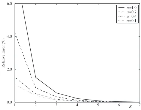
Figure 1. The relative error of Jx component versus numberK of iteration.
1 2 3 4 5 6 7
0.0 2.0 4.0 6.0
Relative Error (%)
a=1.0 a=0.7 a=0.4 a=0.1
K
Figure 2. The relative error of Jy component versus numberK of iteration.
1 2 3 4 5 6 7
0.0 0.4 0.8 1.2 1.6 2.0
Relative Error (%)
a=1.0 a=0.7 a=0.4 a=0.1
K
Figure 3. The relative error of Jz component versus numberK of iteration.
1 5 10 15
0.0 5.0 10.0
Relative Error (%)
Jx Jy J
z
K
Figure 4. The relative error of J components versus numberK of iteration,a= 5.0.
to 0.015% in the seventh iteration. This error diminishes if adecreases. So, at a= 0.1, the values of relative error are equal to 0.52% and 0.004%, respectively. The respective values of the relative error for
Jy component are equal to 8.32% and 0.013% for a= 1.0, and 1.07% and 0.004% for a= 0.1 (Fig. 2). These values for Jz are equal to 2.03% and 0.006% for a = 1.0, and 0.78% and 0.002% for a = 0.1 (Fig. 3). Summarizing these results, one can conclude that exactness of the obtained solutions does not exceed several thousandths of percent; therefore, the values of respective E components will be calculated with guaranteed high accuracy.
In order to determine the region of the applicability of the proposed method of successive approximation, we carry out calculations in wide region of parameter a. It is found that with growth ofa, the iterative procedure becomes somewhat instable, and it becomes divergent at a >10.0. This is explained by the fact that the condition in Eq. (27) does not hold at the givenω and ζ.
In Fig. 4, the behavior of convergence is shown at a= 5.0. One can see that the convergence for
Jy and Jz component is non-monotone. Moreover, the values of relative error are greater than that for small values of a(in the first stage, they are equal to 9.39%, 18.51%, and 7.49% forJx, Jy and Jz
0.0
1.0
2.0
3.0
0.0 2.0 4.0 6.0 0.0 2.0
θ φ
| Jr| a=0.1, p=0.2,
max(|Jr|)=3.8705e-005
Figure 5. Amplitude of Er component of the scattered field,a= 0.1.
0.0
1.0
2.0
3.0
0.0 2.0 4.0 6.0 0.0 0.05
0.1 a max(|J=5.0, p=10.0,
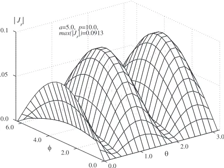
r|)=0.0913
φ
θ | J
r|
Figure 6. Amplitude of Er component of the scattered field,a= 5.0.
as for small a grows twice. So the relative error equal to thousandths of percent is achieved on 15 iteration, and it is equal to 0.008%, 0.007%, and 0.005% for Jx,Jy and Jz components, respectively.
After determination of the area of convergence of the problem’s parameters, one can deal with solving the diffraction problem. The first step consists of solving Eq. (8) by means of passing to LAS corresponding to Eq. (12). Let us consider the case of plane waveE0 =βeikα·x;β is constant vector; α
is unit vector, andα·β = 0. If the components of vector-functionJ are determined, the values of vector
E are determined explicitly by formula (6). For the considered case, vector E has only x-component, and Ey ≡ Ez ≡ 0. In practice, the spherical components of electromagnetic field are of much interest to researchers. In this connection, we pass to the spherical components of field using known formulas (see, for example, [15]). In Fig. 5, the amplitude of Er component is shown for a= 0.1, and the rest of parameters are the same as in the previous example. The field components are calculated at the distance p= 2afrom the particle center.
The electrical size of a particle at such a is small: in our case k = 0.1, therefore total ka = 0.01 that corresponds to very small diameter of scattering, and amplitude of scattered field is fifth order lower than the amplitude of incident field that is equal to 1.0 in our case of plane wave. The maximal value of Er component is equal to 3.87×10⁻⁵; the amplitude diminishes ifp grows. In the case that a
grows, the form of scattered field changes slightly, but the amplitude increases on several orders. For example, this amplitude is equal to 0.0913 ata= 5.0. (see Fig. 6).
5.2. Comparison with Mie Type and Asymptotic Solutions
In order to establish the accuracy of EM field components received by solving LAS for J components and next determining them by formula (6), we compare the received results with Mie type solution received in [2]. Mie type solution is considered here as benchmark one. In Fig. 7, the relative error of our solution is demonstrated for different values of impedance ζ. One can see that relative error grows slightly as ζ increases, but it does not exceed 3×10⁻²% for the considered values of a. In fact, the relative errors are very close forEx, Ey, andEx components; therefore, it is shown for componentEx
only. So, at ζ = 2000, this error is equal to 3.1×10⁻⁵% at a= 0.01, and it grows to 2.7×10⁻²% at
a = 0.05. The relative error diminishes if ζ decreases, equals 2.75×10⁻²% at ζ = 2000, and equals 0.75×10⁻²% at ζ= 500 for a= 0.05.
The numerical calculations carried out for the values ofain the limits from 1.0 to 10.0 for different
0.01 0.015 0.02 0.025 0.03 0.035 0.04 0.045 0.05 x 10⁻⁴
Relative Error
ζ=1000 ζ=500 ζ=2000
a 0
0.5 1 1.5 2 2.5 3
Figure 7. Relative error of new solution forEx
component.
0.01 0.015 0.02 0.025 0.03 0.035 0.04 0.045 0.05
0.0 0.01 0.02 0.03 0.035
Relative Error
ζ=500, Ey
ζ=1000, E
y
ζ=2000, Ey
ζ=500, Ex
ζ=1000, E
x
ζ=2000, Ex
a
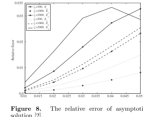
Figure 8. The relative error of asymptotic solution [2].
aand ζ forEx and Ey components. The maximal value of relative error is attained forEx component atζ = 2000 in the pointa= 0.04, and it is equal to 3.3%. The minimal value of error is equal to 0.43%, and it is attained at a= 0.01. The relative errors for Ey and Ez components practically coincide for this case.
The obtained results show that the relative error of asymptotic solution is worse than the relative error in the previous example. In this connection, we compare our new solution with the solution obtained in [34], which is determined by the specified asymptotic formula. This formula contains an additional term taking into account the smallness ofaof the particle radius. It is found that the relative error of this specified asymptotic solution is much better than that for the regular asymptotic solution. In Fig. 9, the relative error of solution obtained in [34] is shown forEx andEy components. As in the previous example, our new solution is considered as benchmark one. The plots demonstrate that relative error for this case is much less than in the previous one, and it is close to the relative error of Mie solution. In total, this error is worse on 0.5×10⁻²% than that for Mie solution. For this case we observe different relative errors for Ex and Ey components only at ζ = 2000. The maximal error is attained forEx component ata= 0.05, and it is equal to 3.9×10⁻²%. The maximal error is attained for
Ey component ata= 0.05, and it is equal to 4.6×10⁻⁴%.The relative errors forExandEy components at ζ = 500 and ζ = 1000 practically coincide, and this error for Ez component coincides with relative error forEy component for all considered ζ. The above results confirm that considering the additional term in the specified asymptotic solution (see [34]) has sense even at large values ofa.
Of course, the proposed method cannot rival those proposed in [34] on the required computing time. The calculation of vector E values is carried out by the explicit formulas (3.3) and (3.4) there. Here, we should calculateE by formula (6) that implies solving integral equation (8) for vectorJ. The main disadvantage is that the elements of matrix A and right part f are respective integrals, and for their calculation we need a lot of time. For example, in [34] one needs about 0.5 sec (taking into account calculation of some preliminary parameters) for calculation E value on PC with CPU 2.4 GHz for the particle with radius a= 0.01 cm,k = 1.0 cm−1, at ζ = 500.0; the calculation by the proposed method needs 1 min, 23.6 sec. However, the first advantage of the last method is that it is applicable to a large set ofavalues.
The second advantage of method is that it can be applied successfully in the range of small wave lengths, because the respective algorithm is sensitive for product a and k only. For small a
and λ(k = 2π/λ) values, ka remains in the limits 1.0×10⁻³ −1.0 (nanometer size of particle and micrometer length of wave, for example) that permits to have a good performance of algorithm in the range mentioned above. The numerical calculations show that the amplitude of scattered field diminishes by the respective law if the radiusaof particle decreases.
0.01 0.015 0.02 0.025 0.03 0.035 0.04 0.045 0.05 0.0
1.0 2.0 3.0
Relative Error
ζ=500, E
x
ζ=500, E
y
ζ=1000, E
x
ζ=1000, E
y
ζ=2000, E
x
ζ=2000, E
y
a 4.0
x10-4
Figure 9. The relative error of specified asymptotic solution [34].
0.01 0.015 0.02 0.025 0.03 0.035 0.04 0.045 0.05
0.0 0.5 1.0 1.5 2.0 2.5
Relative Error
ζ=20, E
x
ζ=20, E
y
ζ=50, E
x
ζ=50, E
y
ζ=80, E
x
ζ=80, E
y
a x10-5
Figure 10. The relative error of specified asymptotic solution [34] for small values ofζ.
can see that the maximal value of relative error is attained for Ex component atζ = 80, and it is equal to 2.2×10⁻³%. The value of relative error for all components at a= 0.01 coincides for all considered
ζ, and it is equal about to 2.5×10⁻⁵%.
Summarizing the presented results, we conclude that the new solution, obtained by solving the Fredholm integral equation with next application of formula (6) is exact enough in the wide range of parameters a and ζ. The relative error in comparison with the Mie type solution does not exceed 3.0×10⁻²%, and relative error of specified asymptotic solution is slightly worse: it does not exceed 4.0×10⁻²%.
5.3. Case of the Ellipsoid Particle
The results, considered in the two previous subsections, concern the case of spherical particle. If we wish to solve the problem for the particle with another geometry, we should take into account the change of the particle form. For example, in the process of numerical solving Fredholm Eq. (8) and LAS respective to it, we should use the actual representation of the element of surface area. So if we pass from investigation of spherical particle to particle in the ellipsoid form, we should change the element of spherical areadt=a2sinθdϕdθ by
dt=
b2c2cos4θcos2ϕ+accos4θsin2ϕ+a2b2sin2θcos2θdϕdθ, (29)
and to take into account that derivative respectively torcoordinate is not equal to zero on the surface of ellipsoid, in contrast to a spherical particle. The numerical results show that properties of convergence of the method of successive approximations are similar to the case of a spherical particle; this method converges very rapidly for the case that the semiaxes of ellipsoid do not differ in the limits of 20%. If this difference grows, the convergence becomes slowly, and we need twice of the number of iterations to achieve the same accuracy as for spherical particle ifb, c≥3a, whereais the value of semiaxis along x
coordinate, b the value of semiaxis along y coordinate, and c the value of semiaxis along z coordinate. The amplitude form of the scattered field does not differ considerably if the semiaxesa, b, cof ellipsoid vary in the limits of 10%.
The numerical results show that amplitude of the scattered field of ellipsoid particle increases more quickly than amplitude of the scattered field of spherical particle while value of semiaxis agrows, and the values b and c remain the same; k = 0.05 m−1. In Fig. 11 and Fig. 12, the comparative results related to change of the amplitude ofEr component are shown for two cases. In the first case (Fig. 11), the value of semiaxis b= 3aand the value of semiaxis c=a. In the second case (Fig. 12), b= 3aand
1.0 2.0 3.0 4.0 5.0 0.0
0.02 0.04 0.06 0.08 0.1
max( |
Er
|)
ζ=50 ζ=200 ζ=500 ζ=50 ζ=200 ζ=500
a
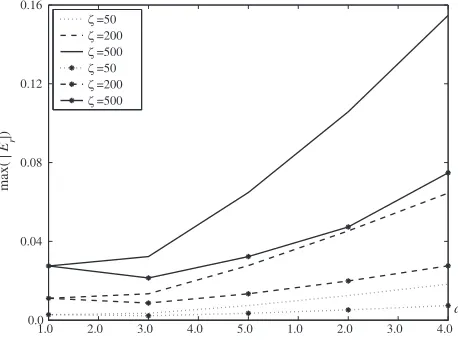
Figure 11. Maximal amplitude ofErcomponent at semiaxes b= 3a, c=a.
1.0 2.0 3.0 4.0 5.0 1.0 2.0 3.0 4.0
0.0 0.04 0.08 0.12 0.16
max( |
Er
|)
ζ=50 ζ=200 ζ=500 ζ=50 ζ=200 ζ=500
a
Figure 12. Maximal amplitude ofEr component at semiaxes b= 3a,c= 3a.
for the second case ata= 5.0. The difference of two amplitudes is the biggest ata= 5.0, and it is equal to 0.063. Increase of amplitude at smaller ζ is not so great. For comparison, the growth of amplitude for the case of spherical particle with the sameais shown by lines marked with asterisk.
The numerical calculations show that the amplitude of scattered field components for the ellipsoid particle tends to the respective amplitude for the spherical particle, if the values of semiaxes b and c
tend to a. This fact confirms the correctness and accuracy of the elaborated method for the case of the ellipsoid particle. The method is generalized for the case of a particle of an arbitrary shape. The main difficulty for such generalization is to elaborate the numerical algorithm for replacement of the analytical representation of the element of area by its numerical analog.
Among a variety of publications, devoted to application of integral equation method to solve EM and acoustic wave scattering problems, one should note the approach proposed in the Chapter “Integral Equation Method for Three-Dimensional Bodies” from book [24], which is closest to our consideration. In [42], the uniform surface integral equation method is applied to the investigation of EM wave scattering by objects with mixed boundary conditions. The obtained set of integral equations is converted to respective LAS using the Galerkin’s technique. The structure of the obtained matrix is similar to the structure of matrix in Eq. (12). Similar to our procedure, the obtained solution is compared with a known Mie type solution for sphere in the near and far zones. The exactness of both the approaches is comparable. The disadvantage of method [42] is that the number of basic functions for sphere with kr = 1.0 and respective discretization needs more than 960 unknowns (this is order of respective LAS). In our case, the order of matrices in Eqs. (25), (26) at such kr is about 200.
The numerical procedure to solve the respective LAS in [41] needs calculation of double series (corresponding to space discretization) that yields in matrices of order 1068 at r= 0.5 m. The method proposed in [44] is more powerful, but it is applicable to scatterers of rectangular form only. In conclusion, one can substantiate that our method is exact, effective, and it can be applied successfully to solve scattering problems in a wide range of particle’s size and frequency band.
6. CONCLUSIONS
ACKNOWLEDGMENT
Author thanks Prof. Alexander G. Ramm, Kansas State University, USA, for creative discussions related to the topic under investigation.
REFERENCES
1. Andriychuk, M. I. and A. G. Ramm, “Scattering by many small particles and creating materials with a desired refraction coefficient,”Intern. Journ. of Computing Science and Mathematics, Vol. 3, No. 1/2, 102–121, 2010.
2. Andriychuk, M. I., S. W. Indratno, and A. G. Ramm, “Electromagnetic wave scattering by a small impedance particle: Theory and modeling,” Optics Communications, Vol. 285, 1684–1691, 2012. 3. Attaran, A., W. B. Handler, K. Wawrzyn, R. S. Menon, and B. A. Chronik, “Reliable RF B/E-field
probes for time-domain monitoring of EM exposure during medical device testing,” IEEE Trans.
Antennas Propagat., Vol. 65, No. 9, 4815–4823, 2017.
4. Barber, P. W. and S. C. Hill, Light Scattering by Particles: Computational Methods, World Scientific, Singapure, 1990.
5. Chen, Y., Y. Ge, G. B. M. Heuvelink, R. An, and Y. Chen, “Object-based superresolution land-cover mapping from remotely sensed imagery,” IEEE Transactions on Geoscience and Remote
Sensing, Vol. 56, No. 1, 328–340, 2018.
6. Faran, J. J., “Sound scattering by solid cylinders and spheres,” J. Acoust. Soc. Amer., Vol. 23, No. 4, 405–418, July 1951.
7. Gensheimer, P. D., C. K. Walker, R. W. Ziolkowski, and C. D. D’Aubigny, “Full-scale three-dimensional electromagnetic simulations of a terahertz folded-waveguide traveling-wave tube using ICEPIC,”IEEE Transactions on Terahertz Science and Technology, Vol. 2, No. 2, 222–230, 2012. 8. Glisson, A. W., “Electromagnetic scattering by arbitrarily shaped surfaces with impedance
boundary conditions,” Radio Sci., Vol. 27, No. 6, 935–943, November 1992.
9. Helander, J., A. Ericsson, M. Gustafsson, T. Martin, D. Sh¨oberg, and C. Larsson, “Compressive sensing techniques for mm-wave nondestructive testing of composite panels,”IEEE Trans. Antennas
Propagat., Vol. 65, No. 10, 5523–5531, 2017.
10. Van De Hulst, H. G., Light Scattering by Small Particles, Dover, New York, 1981.
11. Ishimaru, A., Electromagnetic Wave Propagation, Radiation and Scattering, Englewood Cliffs, Prentice-Hall, NJ, 1991.
12. Kantorovich, L. V. and V. I. Krylov, Approximate Methods of Higher Analysis, Noordhoff, Groningen, 1958.
13. Kaye, M., P. K. Murthy, and G. A. Thiele, “An iterative method for solving scattering problems,”
IEEE Trans. Antennas Propagat., Vol. 33, No. 11, 1272–1279, November 1985.
14. Ko, W. L. and R. Mittra, “A new approach based on a combination of integral equation and asymptotic techniques for solving electromagnetic scattering problems,” IEEE Trans. Antennas
Propagat., Vol. 25, No. 2, 187–197, March 1977.
15. Korn, G. A. and T. M. Korn, Mathematical Handbook for Scientists and Engineers, McGraw-Hill Book Company, 1968.
16. Kyurkchan, A. G. and S. A. Manenkov, “Solving the problem of electromagnetic wave diffraction at a finite plane grating with small elements,” Journal of Quantitative Spectroscopy and Radiative
Transfer, Vol. 180, 92–100, 2016.
17. Landau, L., E. Lifschitz, and L. Pitaevsky, Electromagnetizm of Continuous Medium, Pergamon Press, Oxford, 1984.
18. Lu, K.-Y., S.-C. Tuan, H.-T. Chou, and H.-H. Chou, “Analytical analysis of electromagnetic transient scattering from perfectly conducting ellipsoidal surfaces illuminated by a plane wave,”
Proc. of IEEE International Symposium on Antennas and Propagation (APS-URSI), 2523–2526,
19. Mason, W. P. and R. N. Thurston, “Physical acoustics principles and methods,”Academic, Vol. XV, 191–202, New York, 1981.
20. Medgyesi-Mitschang, L. N. and J. M. Putman, “Integral equation formulations for imperfectly conducting scatterers,” IEEE Trans. Antennas Propagat., Vol. 33, No. 2, 206–214, February 1985. 21. Mie, G., “Beitr¨age zur Optik tr¨uber Medien, speciell kolloidaler Metall¨osungen,” Annalen der
Physik, Vol. 330, No. 3, 377–445, 1908.
22. Mishchenko, M. I., L. D. Travis, and A. A. Lacis,Scattering, Absorption and Emission of Light by
Small Particles, Cambridge University Press, 2002.
23. M¨uller, C., Foundations of the Mathematical Theory of Electromagnetic Waves, Springer-Verlag, Berlin, 1969.
24. Peterson, A. F., S. L. Ray, and R. Mittra,Computational Methods for Electromagnetics, 1st Edition, Wiley IEEE Press, 1977.
25. Poggio, A. J. and E. K. Miller, “Integral equation solutions of three dimensional scattering problems,”Computer Techniques for Electrornagnetics, R. Mittra, ed., Chap. 4, Pergamon, Oxford, 1973.
26. Rao, S., “Innovative antenna front ends from L-band to Ka-band,”IEEE Antennas &Propagation
Magazine, Vol. 59, No. 5, 116–129, October 2017.
27. Rao, S. M., D. R. Wilton, and A. W. Glisson, “Electromagnetic scattering by surfaces of arbitrary shape,” IEEE Trans. Antennas Propagat., Vol. 30, No. 3, 409–418, May 1982.
28. Ramm, A. G., Wave Scattering by Small Bodies of Arbitrary Shapes, World Scientific, Singapure, 2005.
29. Ramm, A. G., “Many-body wave scattering by small bodies and applications,” J. Math. Phys., Vol. 48, No. 10, 103511, 2007.
30. Ramm, A. G., “Wave scattering by many small particles embedded in a medium,” Phys. Lett. A, Vol. 372/17, 3064–3070, 2008.
31. Ramm, A. G., “Electromagnetic wave scattering by many small bodies and creating materials with a desired refraction coefficient,” Progress In Electromagnetics Research M, Vol. 13, 203–215, 2010. 32. Ramm, A. G., “Scattering by many small inhomogeneities and applications,” Topics in Chaotic Systems, Selected Papers from Chaos 2010 International Conference, C. Skiadas, I. Dimotikalis, C. Skiadas, ed., 41–52, World Sci. Publishing, 2011.
33. Ramm, A. G. and M. I. Andriychuk, “Application of the asymptotic solution to EM field scattering problem for creation of media with prescribed permeability,”J. Appl. Math. Comput., Vol. 45, No. 1, 461–85, 2014.
34. Ramm, A. G. and M. I. Andriychuk, “Calculation of electromagnetic wave scattering by a small impedance particle of an arbitrary shape,”Mathematical Modeling of Natural Phenomena, Vol. 9, No. 5, 254–269, 2014.
35. Rylander, T., A. Bondeson, and P. Ingelstr¨om, Computational Electromagnetics, 2nd Edition, Springer, 2012.
36. Sheng, X.-Q., J.-M. Jin, J. Song, C.-C. Lu, and W. C. Chew, “On the formulation of hybrid finite-element and boundary-integral methods for 3D scattering,”IEEE Trans. Antennas Propagat., Vol. 46, No. 3, 303–311, March 1998.
37. Soudais, P., “Computation of the electromagnetic scattering from complex 3D objects by a hybrid FEM/BEM method,”Journal of Electromagnetic Waves and Applications, Vol. 9, No. 7, 871–886, July 1995.
38. Ufimtsev, P. Y., Axially Symmetric Scattering of Acoustic Waves at Bodies of Revolution
(Fundamentals of the Physical Theory of Diffraction), Wiley-IEEE Press, 2014.
39. Vesnik, M. V., “Analytical solution for electromagnetic diffraction on 2-D perfectly conducting scatterers of arbitrary shape,” IEEE Trans. Antennas Propagat., Vol. 49, No. 12, 1638–1644, December 2001.
41. Yang, C. X. and M. S. Tong, “Time-domain analysis of transient electromagnetic scattering from dielectric objects based on electric field integral equations,” IEEE Trans. Antennas Propagat., Vol. 65, No. 2, 966–971, 2017.
42. Yl¨a-Oijala, P., S. P. Kiminki, H. Walln, and A. Sihvola, “Uniform surface integral equation formulation for mixed impedance boundary conditions,”IEEE Trans. Antennas Propagat., Vol. 63, No. 12, 5718–5726, 2015.
43. Yuan, X. C., “Three-dimensional electromagnetic scattering from inhomogeneous objects by the hybrid moment and finite element method,”IEEE Trans. Microwave Theory Tech., Vol. 38, No. 8, 1053–1058, August 1990.