ABSTRACT
HUANG, RONG. The Two-stage Stochastic View Selection Problem in OLAP Systems: Models and Algorithms. (Under the direction of Dr. Rada Chirkova and Dr. Yahya Fathi.)
The Two-stage Stochastic View Selection Problem in OLAP Systems: Models and Algorithms
by Rong Huang
A dissertation submitted to the Graduate Faculty of North Carolina State University
in partial fulfillment of the requirements for the Degree of
Doctor of Philosophy
Operations Research
Raleigh, North Carolina 2013
APPROVED BY:
Dr. Carla Savage Dr. Reha Uzsoy
Dr. Rada Chirkova Co-chair of Advisory Committee
Dr. Yahya Fathi
DEDICATION
BIOGRAPHY
ACKNOWLEDGEMENTS
TABLE OF CONTENTS
LIST OF TABLES . . . vii
LIST OF FIGURES . . . ix
Chapter 1 Introduction . . . 1
1.1 Contributions . . . 6
1.2 Dissertation structure . . . 7
Chapter 2 Related work . . . 9
2.1 Overview of related work . . . 9
2.2 An integer programming method for the one-stage view-selection problem . . . . 13
Chapter 3 The two-stage stochastic view-selection problem . . . 16
3.1 Formulation of the two-stage stochastic view-selection problem SVS . . . 16
3.2 A two-stage stochastic programming modelSP . . . 19
Chapter 4 Solving the stochastic programming model SP . . . 23
4.1 An integer programming model . . . 23
4.2 Reduction of the search space of views . . . 24
4.2.1 First reduction . . . 25
4.2.2 The second reduction . . . 26
4.2.3 The third reduction . . . 27
4.2.4 A reduction algorithm and reduced search spaces of views . . . 28
4.3 Modified integer programming modelIP2 . . . 31
4.4 Experimental results of solving the problemSVS . . . 32
4.4.1 Constructing the instances . . . 33
4.4.2 Reducing the search space . . . 35
4.4.3 Scalability of the model IP2 . . . 38
4.4.4 Summary of observations . . . 39
Chapter 5 Value of the two-stage stochastic model. . . 40
5.1 Two-stage versus one-stage . . . 41
5.2 The value of stochastic solution (VSS) . . . 42
5.3 The expected value of perfect information (EVP I) . . . 45
5.4 Numerical results . . . 48
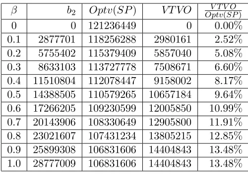
5.4.1 Numerical results on VT VO . . . 48
5.4.2 Numerical results on VSS . . . 52
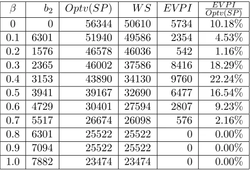
5.4.3 Numerical results on EVP I . . . 57
Chapter 6 The one-stage view-selection problem . . . 60
6.1 The problemOVS and the model OVIP2 . . . 60
6.2 Experimental results on the modelOVIP2 . . . 61
6.2.2 Scalability of the model OVIP2 . . . 65
Chapter 7 A criterion to evaluate a view . . . 67
7.1 The cost-benefit ratio . . . 67
7.2 The minimum cost-benefit ratio . . . 69
Chapter 8 Heuristic methods for the one-stage view-selection problem . . . 74
8.1 The cost-benefit ratio and the modelOVIP2 . . . 74
8.2 Heuristic method I: the single-threshold strategy . . . 77
8.3 Heuristic method II: the two-threshold strategy . . . 78
8.4 Experimental results . . . 81
8.4.1 Experiments with heuristic method I . . . 82
8.4.2 Experiments with heuristic method II . . . 86
8.4.3 Comparison with the inexact model IP V(s) . . . 88
Chapter 9 Heuristic methods for the two-stage problem . . . 91
9.1 The minimum cost-benefit ratio . . . 91
9.2 A heuristic method . . . 92
9.3 Experimental results . . . 94
Chapter 10Concluding remarks . . . 97
10.1 Contributions . . . 97
10.2 Future research . . . 98
10.2.1 Adjusting the “cost-benefit ratio” for the two-stage problem . . . 99
10.2.2 Impact of the datasets . . . 99
10.2.3 Index (and view) selection in the two-stage stochastic setting . . . 99
References. . . .100
Appendices . . . .103
Appendix A Instances of the problem SVS in Section 4.4 . . . 104
Appendix B Synthetic datasets . . . 111
B.1 The symmetric synthetic datasets . . . 111
B.2 Type I non-symmetric synthetic datasets . . . 111
Appendix C Instances of the problemOVS in Section 6.2 . . . 114
Appendix D Details of the instance in Example 9 of Section 8.4.1 . . . 119
LIST OF TABLES
Table 1.1 The Sales table . . . 2
Table 1.2 The Time table . . . 2
Table 1.3 The Customer table . . . 3
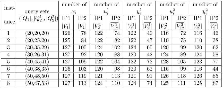
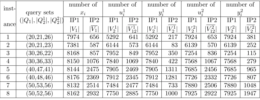
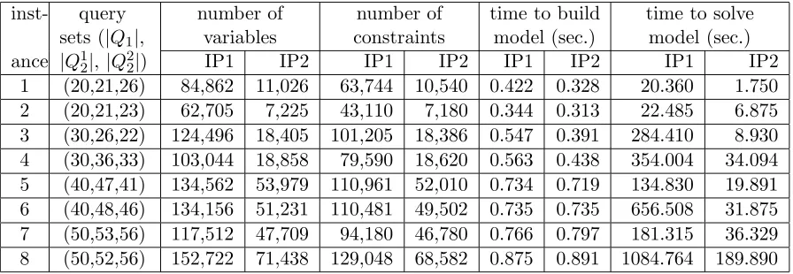
Table 4.1 Comparison of the search spaces of views in the modelsIP1 andIP2, for instances on the 7-attribute TPC-H database . . . 35
Table 4.2 Comparison of the sizes and computing times in the modelsIP1 andIP2, for instances on the 7-attribute TPC-H database . . . 36
Table 4.3 Comparison of the search spaces of views in the modelsIP1 andIP2, for instances on the 13-attribute TPC-H database . . . 36
Table 4.4 Comparison of the sizes and computing times in the modelsIP1 andIP2, for instances on the 13-attribute TPC-H database . . . 37
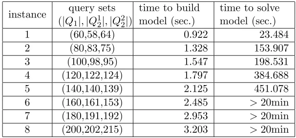
Table 4.5 Scalability ofIP2 for instances on the 13-attribute TPC-H database . . . 38
Table 4.6 Time of solvingIP2 for instances on the 17-attribute TPC-H database . . 38
Table 5.1 Results ofVT VO for Example 2 . . . 51
Table 5.2 Results for VT VO for Example 3 . . . 51
Table 5.3 Values ofVSS for Example 4 . . . 55
Table 5.4 Values ofVSS for Example 5 . . . 56
Table 5.5 Results ofEVP I for Example 6 . . . 58
Table 5.6 Results ofEVP I for Example 7 . . . 58
Table 6.1 Comparison of the numbers of views and the sizes in the models OVIP1, OVIP1′, and OVIP2, for instances on the 17-attribute TPC-H dataset . . 63
Table 6.2 Comparison of the computing times of the models OVIP1′ and OVIP2, for instances on the 17-attribute TPC-H dataset . . . 64
Table 6.3 Scalability ofOVIP2 for instances on the 17-attribute TPC-H dataset . . . 66
Table 8.1 The number of views and the size of the model IP Rv(γ) with different values ofγ for Example 9 . . . 83
Table 8.2 Comparison of the number of views in the search space, of the total exe-cution time, and of the optimal value of the modelsOVIP2 andIP Rv(γ0.2) 85 Table 8.3 The impact of the space-limit parameterλon the choice ofγ for Example 9 85 Table 8.4 Comparison of the number of variables, the number of constraints, and the total execution time in the modelsIP v(γ0.2) and IP Rvq(γ0.2, θ0.2) . . . 86
Table 8.5 Comparison of the total execution time in the models IP Rvq(γ0.2, θ0.2) and IP V(s0.2) . . . 89
Table 8.6 Comparison of the cost value obtained from the modelsIP Rvq(γ∗, θ∗) and IP V(s∗) . . . 90
Table A.1 Description of eight instances on the 7-attribute TPC-H dataset discussed in Section 4.4 . . . 104 Table A.2 Description of eight instances on the 13-attribute TPC-H dataset discussed
in Section 4.4 . . . 107 Table B.1 The symmetric dataset D(3,4) (the relation is shown using four fragments).112 Table B.2 Non-symmetric dataset D(3; 2,3,4) (the relation is shown using two
frag-ments). . . 113 Table C.1 Description of 20 instances on the 17-attribute TPC-H dataset discussed
LIST OF FIGURES
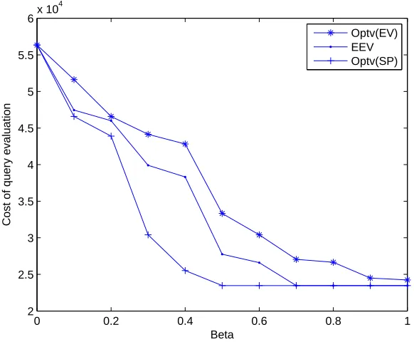
Figure 3.1 View lattice for Example 1, with view sizes shown as number of bytes. . . 18 Figure 5.1 The impact of β (Beta) on the optimal values for Example 2 . . . 50 Figure 5.2 The impact of β (Beta) on optimal values for Example 3 . . . 52 Figure 5.3 The impact of β (Beta) on the values ofEEV and on the optimal values
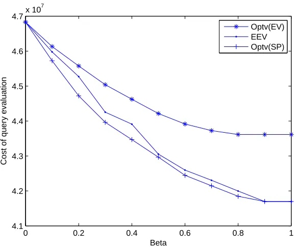
of the models SP andIP EV for Example 4 . . . 54 Figure 5.4 The impact of β (Beta) on the values ofEEV and on the optimal values
of the models SP andIP EV for Example 5 . . . 55 Figure 7.1 The minimum cost-benefit ratios for Example 8 . . . 73 Figure 8.1 The choices of view-query relationships for Example 8 of Section 7.2 . . . 80 Figure 8.2 The execution time and the quality of solutions (gap) of the modelIP Rv(γ)
with different values of γ for Example 9 . . . 84 Figure 8.3 The query-evaluation cost obtained by the model IP Rvq(γ, θ) with
dif-ferent values of γ and θ . . . 87 Figure 9.1 The execution time and the quality of solutions (gap) of the modelIP R2(γ0)
Chapter 1
Introduction
Many data-intensive systems, such as commercial or scientific database systems, store vast collections of data, whose scale tends to grow massively over time. Such systems can improve some metric, such as performance, of answering user queries on stored data by using derived data. Derived data are computed and stored in the system in advance (that is, arematerialized)
using the stored base data, and include cached replicas, indexes, and materialized views, which are used extensively in information integration and data warehouses. Materialized views, that is precomputed and stored extra relations, are commonly used to reduce the evaluation costs of data-analysis queries in relational data-intensive systems. Intuitively, a materialized view would improve the efficiency of evaluating a query when the view relation represents the result of (perhaps time-consuming) precomputation of some subexpression of the query of interest; see [12, 28] and references therein. Materialized views with grouping and aggregation may be especially attractive for evaluating data-analysis queries, because the relations for such views store in compact form the results of (typically expensive) preprocessing of large amounts of data. Selecting appropriate materialized views for use in data-intensive systems may contribute to solutions to the problems of creation, facilitation, visualization, and understanding of the diverse digital content in a variety of circumstances.
As an illustration, consider the following scenario. Large retail companies (such as Sears, Kmart, Target, and WalMart in the USA) all maintain significant-size databases storing infor-mation about ongoing sales transactions. For instance, WalMart is known to maintain database relations whose size is in billions of rows, ortuples.All these companies generally have significant volumes of marketing analysis going on throughout the year. That is, for accounting, reporting, and business-intelligence purposes, each company’s database system undergoes periodic runs of data-analysis queries on the stored information, including the queries for automatically or manually generated daily, weekly, or monthly summary reports. In typical data-analysis, or
Table 1.1: The Sales table
StoreID State ItemID ItemCatergory CustID DateID QtySold
1 NC 1 2 3 1 70
1 NC 3 2 1 2 100
1 NC 3 2 2 3 80
1 NC 4 1 1 1 100
1 NC 4 1 2 4 100
2 NC 1 2 3 2 25
2 NC 2 1 2 3 14
2 NC 4 1 1 3 12
3 SC 1 2 2 1 30
3 SC 1 2 3 4 40
3 SC 2 1 2 1 30
3 SC 3 2 1 2 100
. . . .
Table 1.2: The Time table DateID Day Month Year
1 24 Dec 2012
2 25 Dec 2012
3 1 Jan 2013
4 2 Jan 2013
. . . .
such as sales amount, as a function of some business aspects, called dimensions. For instance, in a daily volume-of-sales query in analyses run for Sears, the dimensions could be item sold,
time of sale, and customer.
Suppose the Sears sales data are stored in relations (i.e., tables) Sales(StoreID, State, ItemID, ItemCatergory, CustID, DateID, QtySold),Time(DateID, Day, Month, Year), and
Customer (CustID, CustType). Suppose also that these relations form astar schema [10], with
Sales as the “fact table” and Timeand Customer as “dimension tables” (see [24]), as shown in Tables 1.1, 1.2, and 1.3, respectively.
Table 1.3: The Customer table CustID CustType
1 Business 2 Individual 3 Individual . . . .
Q1: SELECT ItemCategory, CustType, SUM (QtySold)
FROM Sales NATURAL JOIN Time NATURAL JOIN Customer WHERE Month = ‘December’ AND Year = 2012
GROUP BY ItemCategory, CustType;
Q2: SELECT StoreID, CustType, MAX (QtySold)
FROM Sales NATURAL JOIN Time NATURAL JOIN Customer WHERE Month = ‘December’ AND Year > 2005
GROUP BY StoreID, CustType;
A data-management system evaluating the queries Q1 and Q2 on just the base (i.e., original stored) relations would need to access all the sales information, including the likely large amount of irrelevant data for the salesbefore the reporting period. On the other hand, using derived data could reduce, perhaps significantly, the time to evaluate the queries Q1 and Q2. For instance, using anindex Ithat provides access to all sales events for all sales IDs for a specific month and year would obviate the need to access the irrelevant data for sales in months before (or after) December 2012 for query Q1. Note that evaluating the queries using the index I would still involve examining the sales data at the granularity of individual sales events. Alternatively, the data-management system could reduce the evaluation time of the queriesQ1and Q2by using a
materialized view V1, which is a relation that stores the total sales (V1amt) and maximum sales (V2amt) per item category per customer type per store per month per year, and is expressed in SQL as follows:
V1: SELECT ItemCategory, CustType, StoreID, Month, Year, SUM (QtySold) AS V1amt, MAX (QtySold) AS V2amt FROM Sales NATURAL JOIN Time NATURAL JOIN Customer GROUP BY ItemCategory, CustType, StoreID, Month, Year;
Observe that the queries Q1 and Q2 can be evaluated using a single relation V1 – that is, no
be dramatically shorter than when not usingV1. Note also that the representation of the base data in the materialized viewV1no longer distinguishes between individual items or sales dates. Ideally in such a setting, in order to maximize the efficiency of query processing, all “ben-eficial views”, such as V1 in the example, would be precomputed and stored (materialized). However, typical storage-space and computational constraints on the database system limit the number of views that can be materialized. Naturally, the problem of selecting an appropriate collection of materialized views has to be addressed in the context of the objectives and lim-itations of each setting. This problem is commonly known as the View-Selection Problem. In recent years, a number of researchers have addressed the subject and developed exact and inex-act methods for solving the problem in a one-stage deterministic environment, where all queries are assumed to be known in advance, and in a one-stage probabilistic environment, where we have a probability (frequency) of occurrence associated with each query in a given collection of queries. (See, for instance, [3–5, 16, 19].) In both environments, the problem is addressed in the context of one fixed query workload, and can thus be called theOne-Stage View-Selection Problem.
However, sometimes knowledge of future query workloads may be available, which allows us to choose appropriate views to make advanced preparation for the processing of the future queries. More specifically, sometimes it is necessary to solve the problem of view selection in settings in which we are given some information about query workloads at a future point in time, in addition to the immediate query workloads. In this dissertation we study this problem for relational OLAP systems in a two-stage environment, and propose appropriate models and algorithms for solving the problem.
To illustrate this environment, let us refer to the Sears example described above. While some data-analysis queries would be posed on the Sears’ sales data throughout the year, some of the queries may be run only at certain times of the year. The focus of such seasonally relevant queries could include, for instance: (i) demand for fancy gadgets (such as large-screen TVs) during heavy sales events (such as Black Friday in the USA); (ii) sales of deeply discounted basic household appliances during Christmas sale events; and (iii) August sale events for summertime gear. In such a situation, aside from designing and using derived data to improve the processing performance of the routine queries occurring throughout the year, it would be beneficial to design and use additional derived data in order to reduce the execution time of such seasonal queries as well.
and computational resources, and any savings in this regard translates to better efficiency in the overall operation. Hence, the problem in this context would be to determine the collection of derived data for two or more seasons (stages), so as to answer all the queries in an efficient manner while keeping the total volume of derived data as low as possible. In other words, in this context we need to propose two or more collections of interrelated derived data, so as to minimize the overall query-response time subject to a storage limit on the amount of the derived data produced.
A further complicating factor in this context is the fact that sometimes it is difficult to predict the specific query workload that would become relevant and prominent in a future season (stage). For instance, political, economic, or environmental factors could all have an impact on the nature of the queries that would become relevant in the fixed future stage. This could lead the experts to forecast two or more possible query workloads for that future stage, with a probability associated with each set. This, in turn, would lead to the need to carry out the analysis in a probabilistic environment, where we account for variousscenarios (i.e., query workloads) that may occur in the future.
For instance, in a situation where we deal with only two seasons, we may need to pro-pose a collection of materialized views to answer a given set of queries immediately (these are first-season, or first-stage, queries), and a plan for several collections of views, each collection as-sociated with a possible set of future queries (these are second-season, or second-stage, queries). In such a situation, in order to facilitate and expedite the process of creating the second-stage collections of views, our decision for the first collection of views (that is, the first-stage deci-sion) should be made with consideration for various possibilities (queries) that may occur in the second stage. The idea here is to reuse as many of the first-stage derived data as possible in the second stage.
This leads us to define a view-selection problem in a two-stage probabilistic environment,
with (current) stage 1 and (fixed-season future) stage 2, and propose models and algorithms for solving the problem. Informally, in our Two-Stage Stochastic View-Selection Problem, the inputs include storage limits, a query workload for stage 1, and a collection of query workloads for stage 2 with a probability of recurrence associated with each workload. (The probabilities of the stage-2 query workloads sum up to 1.) The outputat stage 1includes (1) the set of views to be materialized for the stage-1 queries, and (2) for each stage-2 query workload, the set of views that are to be materialized at stage 2 (including those views that will remain around from stage 1) for that query workload. At stage 2, while the time-consuming materialization of the stage-2 views is taking place, those stage-1 materialized views that remain in the system at stage 2 remain around to improve the efficiency of evaluation of stage-2 queries.Not surprisingly, our
As an illustration, suppose that in the Sears example, the queriesQ1 and Q2(given earlier) constituted the stage-1 query workload. We are also given two stage-2 queries: (1) Query Q3
asks for the total sales per item category per customer type per store in NC in January 2013, and (2) Query Q4 asks for the total sales per state in December 2012. Suppose that either Q3
or Q4will occur at stage 2, each with probability 0.5. Then, at stage 1, instead of materializing the view V1 (as given earlier), we can materialize a view V2 that has the total sales per item category per customer type per store per state per month per year, and use it to answerQ1and
Q2. At stage 2, if Q3 occurs, we use V2 to answer it. Otherwise, if Q4 occurs, we answer it by (designing at stage 1 and) materializingat stage 2a viewV3that stores the total sales per state per month per year. The larger-size relation for V2 can be used to evaluate the queries inboth
stages, assuming that Q3 becomes prevalent in stage 2. In contrast, the smaller-size relation forV3 would replaceat stage 2 the larger-size relation for V2, if queryQ4becomes prevalent in stage 2. Here, the use ofV3, rather than ofV2, would result in a more efficient evaluation of the query Q4.
This example illustrates that our two-stage approach is more efficient and less resource intensive than the one-stage approach to view selection. Indeed, as we show in this dissertation, if we apply a one-stage solver to materialize views only at stage 1, then a greater portion of the materialized views would tend to be irrelevant at stage 2. On the other hand, applying a one-stage solver at each of the two stages would result in creating large volumes of views at stage 2, which could be unnecessarily resource intensive.
Note also that our two-stage approach to view selection is applicable to, and sufficient for, solving multi-stage view-selection problems. The reason is, the view selection takes place during the first season, and when it comes to the second season, any modification of the set of views with respect to the new season will have been applied. During the second season, we can employ this two-stage approach for view selection for the second and third seasons, and so on.
1.1
Contributions
In this dissertation, we introduce the two-stage stochastic view-selection problem and propose an approach for solving the problem. Our approach is to develop a stochastic programming (SP) model for it. More specifically, we show that the SP model that we propose in its extended form is equivalent to an integer programming (IP) model. In general, this IP model may have a large number of variables and constraints. We use the structural properties of the models to reduce the size of the search space of views, and hence the size of the corresponding IP model, to manageable levels. Our specific contributions are as follows:
problem as a two-stage stochastic programming (SP) model in Section 3.2.
2. In Section 4.1 we study the structure and properties of the extensive form of the SP model, which is an integer programming (IP) model. In Section 4.2 we develop an algorithm that effectively reduces the search space of potentially beneficial views in the IP model, and obtain a smaller IP model in Section 4.3 (called “the reduced IP model”) whose solution is guaranteed to be optimal for the original SP model.
3. In Section 4.4 we conduct a computational experiment on the above IP models and discuss the scalability of the reduced IP model. The reduced search spaces significantly reduce the size of our original IP model. As a result, for realistic-size instances of the problem, this IP model can be solved efficiently by a commercial IP solver such as CPLEX [21]. 4. In Sections 5.1-5.4 we compare our two-stage SP model with associated or related models,
and present techniques to assess the value of the SP model and the value of perfect information [6] in this context.
5. In Section 6.1 we introduce an exact method and an integer programming model to solve the one-stage deterministic view-selection problem. We show through a numerical experiment in Section 6.2 that our algorithm outperforms the one introduced in [3, 4]. 6. In Sections 7.1 and 7.2 we study the properties of the views that appear in the optimal
solution in the context of the one-stage view-selection problem. We propose a measure of effectiveness (called cost-benefit ratio) associated with each candidate view, and use this measure to devise heuristic algorithms for solving larger instances of the problem in Sections 8.1-8.3. We demonstrate the effectiveness of our algorithms through a computa-tional experiment in Section 8.4. Our experiment shows that on average, our algorithms require less execution time than the heuristic methods proposed in [3,4], and the resulting solutions are significantly better (i.e., have lower costs).
7. In Sections 9.1 and 9.2 we discuss how this cost-benefit ratio can be employed to devise other heuristic algorithms for solving large-size instances of the two-stage stochastic view-selection problem. In Section 9.3 we conduct a computational experiment to discuss the effectiveness of this algorithm.
1.2
Dissertation structure
Chapter 2
Related work
2.1
Overview of related work
The general view-selection problem has been studied in the literature with various objectives and constraints (see [33] for a survey and the design goals of the problem). In the one-stage deterministic view-selection problem, the goal is to select a set of views to materialize from scratch for answering a given set of queries with associated frequencies of occurrence. Numerous algorithms are proposed for the selection of materialized views in the conventional one-stage form of the problem (see [18] for a survey). Significant work has also been done on index selection in such settings, both on its own and alongside view selection, see, e.g., [1, 2, 7, 8, 11].
Work including [17, 19, 30] consider greedy methods for efficiently selecting views in a gen-eralization of the OLAP setting. Harinarayan et al. in [19] present greedy algorithms for the one-stage view-selection problem in data cubes under a disk-space constraint. To minimize the sum of query and update cost under storage space constraint, Gupta et al. in [17] extend the greedy algorithm of [19] in the selection of data-warehouse materialized views. They introduce “AND-OR” view graphs to represent all possible ways to generate warehouse views, and provide several greedy heuristics for different types of “AND-OR” view graphs. Unfortunately, in [23], Karloff and Mihail disprove the strong performance bounds of these algorithms, by showing that the underlying approach of [19] cannot provide the stated worst-case performance ratios unless P=NP. To minimize query costs under a space constraint, Nadeau et al. in [30] also give a greedy algorithm, which is polynomial in the number of dimensions. That algorithm does not perform as well as other greedy heuristics.
space or update cost.
Considerable work, including [3–5,31,38], has been done in the open literature that employs integer programming (IP) models to obtain optimal selection of derived data for query process-ing in a one-stage environment. Yang et al. [38] propose an integer programmprocess-ing (IP) model for view selection. The model uses Multiple View Processing Plans (MVPPs) to minimize the combined cost of query evaluation and view maintenance. The solution of the IP model can guarantee optimality. However, the algorithm does not take the space constraint into account. In [31] Papadomanolaskis et al. propose an Integer Linear Programming (ILP) model for index selection, with the objective of minimizing the query and update costs under a storage-space constraint for a given collection of queries using a given set of tables. Golfarelli et al. in [15] investigate the benefits of materializing views in vertical fragments in order to minimize the response time of query workloads under a disk-space constraint. Each vertical fragment in-cludes a subset of the measures possibly taken from one or more views, aggregated on the same grouping set. They formulate the problem as an ILP model, and solve it using a standard IP solver. A line of past work [3–5] has focused on formal approaches for selection of views (with or without indexes) to minimize the cost of query processing under the storage-space constraint. Asgharzadeh Talebi et al. propose IP models to address the problem of view selection in [4], and the problem of combined view and index selection in [3, 5]. The objective in both papers is to minimize the query-processing costs under space constraints in a deterministic environment. In both cases, they propose algorithms to effectively and efficiently prune the search space of potentially beneficial views and/or indexes. They develop both exact and inexact methods for solving the problems efficiently. The exact methods of their work guarantee the optimality of the solutions. The results of that work are scalable to relatively large instances of the problem, and compare favorably with several other approaches in the literature, including [2,19,22]. However, those integer linear programming techniques are limited to the problems in the one-stage envi-ronment. To the best of our knowledge, there is no known algorithm that addresses the problem in a multi-stage probabilistic environment. The SP and IP models presented in this dissertation are most closely associated with the models discussed in [3, 4]. We extend these models and approaches to the two-stage deterministic and probabilistic environments. In Section 2.2, we provide a brief introduction of the IP model and methods proposed in [3, 4] for the one-stage view-selection problem. In this dissertation we also extend further the reach of the approach of [3–5] for solving the one-stage view-selection problem, by studying the structural relation-ship between the views and the queries. These results lead us to more effective techniques and algorithms for the problem.
prob-lem discussed in this dissertation, in that they both consider the selection of materialized views for incoming queries over time periods. At the same time, there are also fundamental differences between these paradigms, as described below.
There are a number of solutions, including [7, 8, 25, 26], for the dynamic view-selection problem in the context of periodical “re-calibration” of the materialized views to optimize query-evaluation costs with changes in the query patterns. In [25, 26], Kotidis et al. present DynaMat, a system that dynamically materializes information at multiple levels of granularity, in order to match the query workload under the update and space constraints. DynaMat con-stantly monitors incoming queries, and materializes the best set of views subject to the space constraints. During updates on the stored data, DynaMat reconciles the current materialized views and refreshes the most beneficial subset within a given maintenance window. At the same time, DynaMat can only choose to store aggregate data that are answers to the queries from the users. As a result, even though an aggregate view that can answer multiple aggregate queries may save a lot of space without losing much efficiency in answering these queries, it will never be considered by DynaMat unless it is queried. Our approach in this dissertation allows any aggregate view that can answer any of the queries to be considered for materialization.
In [34,35], Theodoratos et al. consider what they call dynamic or incremental data warehouse design, where new queries are added and need to be answered by a data warehouse. In the first phase (stage), they are given a fixed set of queries Q, and views that answer the queries with minimum cost must be selected from multi-query AND/OR-DAGs. In the second phase (stage), an incoming query workload is given, and another set of materialized views is added to the existing set of views, so that all the incoming queries and the existing queries can be answered. However, in practice there may not be extra space available for materializing new views. In this dissertation, we always require the space for storing materialized views at each stage to be no more than a given space limit.
problem dynamically, in the sense that their algorithm assumes no knowledge of the second-stage queries during the first second-stage. They consider the second-second-stage queries in a deterministic sense, only after the first-stage views are materialized and employed, and solve the two stages of the problem separately. As a result, a great portion of the materialized views M obtained from the startup (first) phase tends to be irrelevant in the online (second) phase, since many of the first-stage queries are no longer of interest in the second phase. In [27], in order to select views for the two phases of the problem, the authors apply the greedy algorithm proposed by Harinarayan et al. in [19] and three randomized methods proposed by Kalnis et al. in [22]. However, these methods do not guarantee optimality of the solution.
The stochastic seasonal view-selection problem proposed in this dissertation differs from dynamic view selection, in that for the stochastic seasonal view-selection problem it is natural to only consider a two-stage (two-season) view selection. The reason is that the selection of views takes place between two seasons, and when it comes to the second season, any modification of the set of views with respect to the new season will be applied. At the end of the second season, we can employ this two-stage approach for view selection between the second and third seasons, etc.
However, none of the work for the multi-stage view-selection problem has been considered in a probabilistic environment. To the best of our knowledge, Shaman [14] is the only project described in the open literature that considers using derived data to improve query performance in presence of a number of distinctly identifiable query workloads, all of which are known before-hand. Our work in this dissertation complements the agenda of Shaman, in that in Shaman, the specific query sets are not tied to specific time points or to particular occurrence probabilities. The objective of the Shaman approach is to set up one initial and, at the same time, final index configuration that would be “robust” in some sense through all the deterministic changes in the query workloads on the system, regardless of when the workload changes are to occur. This approach does not appear to be appropriate for a probabilistic-environment problem, such as the one considered here.
2.2
An integer programming method for the one-stage
view-selection problem
In this subsection, we provide a brief introduction of the models and methods proposed in [3,4] for the one-stage view-selection problem. The models and algorithms that we propose in this dissertation for the two-stage view-selection problem are closely related to these for the one-stage models and methods.
In [4], Asgharzadeh Talebi and colleagues consider the following One-Stage View-Selection problem, which we denote by OVS in this dissertation: Assume we are given a collection of queries Q, with associated frequency distribution on a given star-schema data warehouse D, and a storage limit bon the total size of the views that we may materialize. The problem is to select a collection of views to materialize, so as to minimize the total evaluation costs of the given collection of queries.
The scope of the two-stage view-selection problem which we propose in this dissertation, i.e., the type of the database, as well as the type of queries and views, is the same as in the problemOVS. Hence, we provide a brief introduction here; please see Section 3.1 for a detailed description. For the problem OVS we consider star-schema data warehouses [9, 10, 24] with a single fact table and several dimension tables. All the views to be materialized are defined, with grouping and aggregation but without selection, on the relation that is the result of the “star-schema join” [24] of all the relations in the “star-schema. This relation is called theraw-data viewor
raw-data table. All the queries in the workloads in the problem OVS are posed on the relevant raw-data view. The query-evaluation cost is defined in the context of answering unnested select-project-join queries with grouping and aggregation using unindexed materialized views, such that each query can be evaluated using just one view and no other data. A query can be answered using a view only if the set of grouping attributes of the view is a superset of the set of attributes in the GROUP BY clause of the query and of those attributes in the WHERE clause of the query that are compared with constants. Each query (or view) is represented by the set of these relevant attributes. The evaluation cost of a query using a given view (if this view can indeed be used to answer the query) is equal to the size of the materialized view itself. Please see Section 3.1 for detailed size calculations and estimation of the views or queries.
Thesearch space of views(i.e., the collection of candidate views we consider) for the problem
OVS is the view lattice introduced by Harinarayan et al. in [19], which includes all the views with grouping and aggregation defined on the raw-data table. Each lattice view has grouping on some of the attributes of the database, and has aggregation on all the attributes aggregated in the input queries.
V denote the search space of views for a given problem OVS with a query set Q. Let I and
J denote the set of subscripts associated with the sets V and Q, respectively. For each i ∈ I
we usevi to represent both the ith view in V and the collection of grouping attributes for this
view. Similarly, for eachj ∈J we useqj to represent both thejth query inQand the collection
of attributes in theGROUP BYclause of that query, plus those attributes in theWHERE clause of the query that are compared with constants. Let ai denote the size of the viewvi, for alli∈I.
Letdij be the evaluation cost of answering queryqj using viewvi, for allj∈J and for alli∈I.
Define the decision variables xi andzij for all j∈J and for alli∈I, as follows:
xi =
(
1 if viewvi is materialized
0 otherwise
zij =
(
1 if we use view vi to answer query qj
0 otherwise
The problem OVS can now be formulated as the following integer programming (IP) model, denoted by OVIP1. We use the notation Vj, for every query qj, to represent the collection of
views each of which can be used to answer the query qj, i.e., Vj = {v ∈ V : v ⊇ qj}. In the
model OVIP1 we useIj to denote the set of subscripts inVj.
(OVIP1) minimize X
j∈J
X
i∈Ij
dijzij (2.1)
subject to X
i∈I
zij = 1 ∀j ∈J (2.2)
zij ≤xi ∀j ∈J,∀i∈Ij (2.3)
X
i∈I
aixi ≤b (2.4)
All the variables are binary (2.5)
Constraint (2.2) states that each query is answered by exactly one view; constraint (2.3) guar-antees that a query can be answered by a view only if the view is materialized. Constraint (2.4) limits the storage space for the views to be materialized.
Asgharzadeh Talebi et al. [3, 4] propose to reduce the size of the search space of views (that is, to prune the search space of views) from the view latticeV to a smaller subset based on the following two observations:
Observation 2. There exists an optimal solution for an instance of the problemOVS in which viewv is not materialized, and hence can be removed from the search space of views, if v is not equal to any query in the given query set Q, and the size of v is greater than or equal to the total size of queries it can answer.
As mentioned in Asgharzadeh Talebi et al. [3, 4], these observations allow us to remove a certain number of views at the outset, thus reducing the size of the corresponding model
OVIP1. We can still guarantee that an optimal solution of the reduced model, which we denote by OVIP1′, is also optimal for the original problem OVS. This, in turn, allows us to solve larger instances of the problem and to obtain the corresponding optimal solutions. Through a comprehensive computational study, Asgharzadeh Talebi et al. [3, 4] show the effectiveness of this approach in solving relatively large instances of the problem OVS.
In order to further prune the search space of candidate views, and hence the size of the corresponding IP model, Asgharzadeh Talebi et al. in [3,4] present an inexact (heuristic) method for solving the problemOVS. The basic idea of the inexact method proposed in [3,4] is to limit the search space of views only to those views that are “relatively close” ancestors of the given queries. A view (or query) v1 is an ancestor for another view (or query) v2 if the collection of attributes that definev2 is a proper subset of the collection of attributes that definev1; in this context we refer tov2 as the child (or descendant) ofv1. More specifically, Asgharzadeh Talebi et al. [3] define a setVs as a reduced search space of views with respect to a given parameters,
where each view inVsis the union of exactly 1, or 2, . . ., or squeries in the given query setQ.
Chapter 3
The two-stage stochastic
view-selection problem
In this chapter we define the scope of the two-stage stochastic view-selection problem that we consider, i.e., the type of the databases, queries and views. Subsequently, we propose a stochastic programming (SP) model [6] for this problem. By studying the properties of the SP model, we then rewrite it equivalently as a model with fewer variables and constraints.
3.1
Formulation of the two-stage stochastic view-selection
prob-lem
SVS
usev to represent both a view and the collection of grouping attributes for that view, and we useq to represent both a query and the collection of attributes in theGROUP BYclause of that query, plus those attributes in theWHEREclause of the query that are compared with constants. It follows that queryq can be answered by materialized view v if and only ifq ⊆v.
To evaluate a query using a given view (if this view can indeed be used to answer the query), we have to scan all rows of this view. Hence, the corresponding evaluation cost is equal to the size of the materialized view itself; a similar cost calculation is used in [4,19,22,32,38]. One way to estimate the view sizes in practice, as suggested in the literature, is by getting a relatively small-size sample of the raw-data view and by then evaluating the view definitions on that table, with a subsequent scaleup of the sizes of the resulting relations. We useai to denote the
(estimated) size of each view vi in the problem input. We also use the parameter dij to denote
the evaluation cost of answering query qj using view vi. It follows that for each query qj we
have dij =ai if qj ⊆vi, and we setdij = +∞ otherwise, implying that qj cannot be answered
by the view vi.
In this environment we have a query workload Q1 that we must answer at the present time (stage 1), and a second query workload Q2 that occurs at a future point in time (stage 2). We assume that the query workload Q1 is known and given, but that the second query workload Q2 is a random set with a given probability distribution function. (We use boldface to emphasize that Q2 is a random set, and to differentiate it from a deterministic set such as
Q1.) We illustrate all of these notions in Example 1 later in this subsection.
At stage 1, we materialize a collection of viewsS1 and use these views to answer the queries in Q1. We assume that we have a storage limit b1 for these views (that is, the total size of the views selected must not exceed b1). At stage 2, once the actual collection of queries Q2 for this stage is known, we allow for a partial replacement of some of the view relations that we constructed at stage 1, in order to obtain the collection of views S2 for answering the query set Q2. (Note thatQ2 represents a realization of the random setQ2.) In other words, for each query set Q2, we need a replacement plan, that is, at the end of stage 1 we keep some of the view relations that we materialized at stage 1, to be used again at stage 2 for Q2, while we discard other view relations from stage 1 and replace them with new view relations. We assume that the total size of the views that we replace must not exceed a given storage limit b2. We refer to this space limit as the replacement space limit. Naturally, b2 ≤b1.
In this context, the technical problem that we need to address prior to stage 1 is to select all views in the set S1 and a replacement plan associated with each possible realization Q2 of Q2. The objective is to minimize the total evaluation costs for the queries at stage 1, plus the expected total evaluation costs for the queries at stage 2. Note that in order to obtain a globally optimal solution for this problem, which we call theStochastic View-Selection (SVS)
Figure 3.1: View lattice for Example 1, with view sizes shown as number of bytes.
for every possible realization Q2 of Q2) must be made prior to stage 1.
The search space of views that we consider for a given problem SVS is the view lattice
introduced by Harinarayan et al. in [19]. The view lattice includes all the views defined on the raw-data table, such that each view has aggregation on all the attributes aggregated in the input queries. In the view lattice, each node represents a view, and a directed edge from node v1 to node v2 implies that v1 is a parent of v2, that is, v2 can be obtained from v1 by aggregating over one attribute of v1. To illustrate, we present the following numeric example for a data cube [19] with 4 attributes.
Example 1. Given a database with four grouping attributes a, b, c and d, the view lattice defined in [19] is shown in Figure 3.1. The space requirement for each view in the lattice is given next to its corresponding node. In this instance, we assume that at stage 1, we are given three queries q1 = {a, b}, q2 = {b, c}, and q3 = {c, d}. At stage 2, q4 = {b} and q5 = {a, c} would occur in one query set with probability 0.5, while q6 = {c} and q7 = {b, d} would occur in the other query set with probability 0.5. Equivalently, Q1 = {a, b},{b, c},{c, d} ,
3.2
A two-stage stochastic programming model
SP
In this subsection, we describe a stochastic programming model for the above two-stage stochas-tic view-selection problem (SVS). Although the general form of the model that we propose is valid for any probability distribution function for Q2, in the following model and throughout the rest of this dissertation we assume that Q2 is a random query set with L possible values. More specifically, we assume that Q2 equals query set Qℓ
2 with probability pℓ, for ℓ = 1 toL,
withPLℓ=1pℓ = 1. We refer to each collection of queries Qℓ2 as ascenario. We start by defining the decision variables. For the first stage we define the following decision variables for each view
vi∈V (whereV is the set of all views) and for each queryqj ∈Q1.
xi =
(
1 if viewvi is materialized at stage 1
0 otherwise
zij =
(
1 if we use view vi to answer query qj at stage 1
0 otherwise
For the second stage, we define the following decision variables for each viewvi ∈V and for
each queryqj ∈Qℓ2, for ℓ= 1 toL.
uℓ i =
(
1 if viewvi is materialized at stage 1 and used at stage 2 for query setQℓ2
0 otherwise
yℓ i =
(
1 if viewvi is materialized at stage 2 for query set Qℓ2 0 otherwise
tℓ ij =
(
1 if we use view vi to answer query qj in the query set Qℓ2 at stage 2 0 otherwise
The cardinality of the view setV is 2K, whereKis the number of distinct grouping attributes
in the database. Let I = {1,2, . . . ,2K} be the set of subscripts for all the views v
i ∈ V. In
addition, let J1 be the set of subscripts for all the queries qj ∈ Q1, and let J2ℓ be the set of subscripts for all the queries qj ∈ Qℓ2, for ℓ = 1,2, . . . , L. The problem can now be written as
the following stochastic programming model [6] that we denote bySP.
(SP) minimize X
j∈J1
X
i∈I
dijzij +EQ2Ψ(x,Q2) (3.1)
subject to X
i∈I
zij = 1 ∀j∈J1 (3.2)
zij ≤xi ∀j∈J1 and ∀i∈I (3.3)
X
i∈I
aixi ≤b1 (3.4)
Here, EQ2 denotes the mathematical expectation of response time at stage 2 with respect to Q2. If the probability distribution ofQ2 is as above, we have that
EQ2Ψ(x,Q2) =
L
X
ℓ=1
pℓΨ(x, Qℓ2) (3.5)
where Ψ(x, Q2) is the minimum response time for a given set of values of the first-stage variables x= x1,· · ·, x|V| and for a realization of the second-stage queriesQ2. For each value of ℓ, the corresponding value of Ψ(x, Qℓ
2) is obtained by solving the following view-selection problem. Ψ(x, Qℓ2) = minX
j∈Jℓ
2
X
i∈I
dijtℓij (3.6)
subject to X
i∈I
tℓij = 1 ∀j∈J2ℓ (3.7)
tℓij ≤uℓi +yiℓ ∀j∈J2ℓ and ∀i∈I (3.8)
uℓi ≤xi ∀i∈I (3.9)
X
i∈I
aiyℓi ≤b2 (3.10)
X
i∈I
ai(uℓi +yℓi)≤b1 (3.11)
All the variables are binary (3.12)
Constraints (3.2) and (3.7) state that each query is answered by exactly one view in the set of materialized views. Constraints (3.3) and (3.8) guarantee that a query can be answered by a view only if the view is already materialized. Constraints (3.4), (3.10), and (3.11) state the storage limits on the view sets. Constraint (3.9) guarantees that the view kept from stage 1 to stage 2 is already materialized at stage 1.
In defining decision variables in the above model, we used the subscript ito represent view
vi, and in every case we defined the decision variables for all values ofi in the subscript set I
(or, equivalently, for all views in the entire view setV). Naturally, in practice for each decision variable with a subscript i (associated with view vi), we only need to consider those views vi
that are relevant in the context of that decision variable. For instance, in defining the decision variable xi at stage 1, we only need to define this variable for those views vi that can be used
to answer at least one query either in the first stage or in the second stage. In other words, we need not consider viewvi (or define the corresponding variablexi) if this view is not a superset
Let Qb =Q1∪∪Lℓ=1Qℓ2 be the collection of all queries either in stage 1 or in stage 2. We define
V1 =
n
vi ∈V :vi⊇q for someq∈Qb
o
(3.13)
V2ℓ = nvi ∈V :vi⊇q for someq∈Qℓ2
o
, ℓ= 1, . . . , L (3.14)
Correspondingly, we define the sets of subscripts associated with V1 and V2ℓ as I1 and I2ℓ, for
ℓ= 1 toL, respectively. It follows thatV1 is the set of views that are relevant for stage 1, and
Vℓ
2 is the set of views that are relevant for theℓth sub-problem (scenario) in stage 2, for ℓ= 1 to L.
Similarly, for each query qj in the sets Q1 and/or Qℓ2, we define a sub-collection of views that are relevant in answering that particular query. For each query qj ∈ Q1 we define V1j =
{vi ∈V1:vi ⊇qj}, and for each queryqj ∈Qℓ2 we defineV2ℓj =
vi ∈V2ℓ :vi⊇qj , forℓ= 1 to
L. Again, corresponding to the view setsV1j and V2ℓj we define the associated sets of subscripts
asI1j andI2ℓj, forℓ= 1 to L, respectively.
Example 1 (Continued). In order to defineV1,V21 andV22, we only consider the views that could answer at least one query in the query set Qb = {q1, q2, q3, q4, q5, q6, q7}, Q12 and Q22, respectively. (ForQ12 and Q22, see the first part of this example in Section 3.1.) Thus, we obtain that
V1={b},{c},{a, b},{a, c},{b, c},{b, d},{c, d},{a, b, c},{a, b, d},{a, c, d}, {b, c, d},{a, b, c, d}
V21 ={b},{a, b},{a, c},{b, c},{b, d},{a, b, c},{a, b, d},{a, c, d},{b, c, d},{a, b, c, d}
V22 ={c},{a, c},{b, c},{b, d},{c, d},{a, b, c},{a, b, d},{a, c, d},{b, c, d},{a, b, c, d} .
For each query, we define the relevant view sets in answering that particular query. For example, for the query q1 ={a, b} ∈Q1 we define V11 ={a, b}, {a, b, c}, {a, b, d}, {a, b, c, d} , and for the query q6 ={b, d} ∈Q22 we defineV262 =
{b, d}, {a, b, d}, {b, c, d},{a, b, c, d} .
We can now define the first-stage decision variables xi only for the views in the setV1, and the first-stage decision variableszij only for the viewsvi in the set V1j. Similarly, we can define
the second-stage decision variables uℓ
i andyℓi, only for the viewsvi ∈V2ℓ, and the second-stage decision variables tℓ
ij, only for the views vi ∈ V2ℓj, for ℓ= 1 to L. It follows that we can now
by SP′.
(SP′) minimize X
j∈J1
X
i∈I1j
dijzij+EQ2Ψ(x,Q2) (3.15)
subject to X
i∈I1j
zij = 1 ∀j∈J1 (3.16)
zij ≤xi ∀j∈J1 and ∀i∈I1j (3.17)
X
i∈I1
aixi ≤b1 (3.18)
All the variables are binary (3.19)
The corresponding second-stage subproblem can be written as follows: Ψ(x, Qℓ2) = minX
j∈Jℓ
2
X
i∈Iℓ
2j
dijtℓij (3.20)
subject to X
i∈Iℓ
2j
tℓij = 1 ∀j ∈J2ℓ (3.21)
tℓij ≤uℓi+yℓi ∀j∈J2ℓ and ∀i∈I2ℓj (3.22)
uℓi ≤xi ∀i∈I2ℓ (3.23)
X
i∈Iℓ
2
aiyℓi ≤b2 (3.24)
X
i∈Iℓ
2
ai( uℓi+yℓi)≤b1 (3.25)
Chapter 4
Solving the stochastic programming
model
SP
We begin this chapter by introducing an integer programming model [37] obtained from the extensive form [6] of the stochastic programming model that we introduced in Section 3.2. Later in this chapter, we will study the properties of this integer programming model, use these properties to remove some variables and constraints, and obtain a model that in many cases tends to be significantly smaller. Optimal solutions of the resulting model are guaranteed to be optimal for the original model SP. This, in turn, allows us to solve larger instances of the problem SVS.
4.1
An integer programming model
(IP1) minimize X
j∈J1
X
i∈I1j
dijzij + L
X
ℓ=1
pℓ
X
j∈Jℓ
2
X
i∈Iℓ
2j
dijtℓij (4.1)
subject to X
i∈I1j
zij = 1 ∀j ∈J1 (4.2)
zij ≤xi ∀j∈J1,∀i∈I1j (4.3)
X
i∈I1
aixi ≤b1 (4.4)
X
i∈Iℓ
2j tℓ
ij = 1 ∀j∈J2ℓ, ℓ= 1, . . . , L (4.5)
tijℓ ≤uℓi+yiℓ ∀j∈J2ℓ,∀i∈I2ℓj, ℓ= 1, . . . , L (4.6)
uℓi ≤xi ∀i∈I2ℓ, ℓ= 1, . . . , L (4.7)
X
i∈Iℓ
2
aiyℓi ≤b2, ℓ= 1, . . . , L (4.8)
X
i∈Iℓ
2
ai(uℓi +yiℓ)≤b1, ℓ= 1, . . . , L (4.9)
All the variables are binary (4.10)
Note that for an instance with K attributes, with n1 queries in Q1 at stage 1 and with nℓ2 queries inQℓ
2 at stage 2, forℓ= 1, . . . , L, there are at most (n1+PℓL=1nℓ2+ 2L+ 1)|V1|variables and at most (n1+PLℓ=1nℓ2+ 2L)(|V1|+ 1) + 1 constraints in the integer programming model
IP1, where V1 is as defined in Section 3.2. Thus, even for relatively small values of K, L, n1 andn12, . . . , nL
2, the size of the model could be very large, and the execution time of solving the IP model could be excessively long even with a relatively fast IP solver such as CPLEX 11 [21]. The applicability of our model is thus limited to smaller-size instances. We thus endeavor to reduce the size of our model by reducing the size of the view sets V1, V1j, V2ℓ and V2ℓj, for
ℓ= 1, . . . , L. In Section 4.4, we will provide numerical results for solving the modelIP1.
4.2
Reduction of the search space of views
In this subsection, we make a few observations regarding the properties of the views that appear in an optimal solution for a given problem SVS. Based on these observations, we identify the reduced search spaces of views, which are relatively small subsets of the view sets V1,V1j, V2ℓ
and Vℓ
2j. The reduced search spaces are guaranteed to contain at least one set of the optimal
and obtain an integer programming model that we denote by IP2.IP2 is significantly smaller thanIP1, and optimal solutions of IP2 are guaranteed to be optimal for the modelSP.
4.2.1 First reduction
As introduced in Section 2.2, in a one-stage view-selection problem, Asgharzadeh Talebi et al. [3, 4] propose to reduce the search space of views (i.e., the set of views to consider) by the results of Observation 1 in Section 2.2. In other words, they eliminate from the search space each view v that has at least one attribute that is not in any of the queries answerable by v. We extend this pruning method to our problem SVS as follows.
Given a view v and a set of queries Q, let Q(v) denote the set of queries in Q that v can answer, i.e., Q(v) ={q∈Q:q ⊆v}. We make the following observations.
Observation 3. In an instance of problem SVS, given a view v in the view set V1, if the
number of attributes ofv is strictly greater than the number of attributes in the union set of the queries in Qb thatv could answer, that is,|v|>| ∪q∈Qb(v)q|, then there exists an optimal solution in which v is not materialized at stage one, or equivalently, the corresponding decision variable has the value xi = 0.
Proof. If q could be answered by v, then the set of attributes for q is a subset of that for v, i.e., q ⊆ v. Thus,∪q∈Qb(v)q ⊆v and | ∪q∈Qb(v)q| ≤ |v|. If | ∪q∈Qb(v)q|< |v|, then v has at least one attribute, call it attribute a, that is not in any q ∈ Qb such that q ⊆ v. If there exists an optimal solution in which v is materialized at stage one, we replace it with view v′ =v\ {a}. Since the size of v′ is no more than that ofv, the replacement will not violate the space limit. For each queryq ∈Qb that is answered byv in the optimal solution,q could be answered byv′
with the cost that does not exceed that ofv. Thus, we obtain an optimal solution in whichv is not materialized at stage one, and the corresponding decision variable has the valuexi = 0.
Observation 4. In an instance of problem SVS, given a view v in the view set Vℓ
2, if the
number of attributes of v is strictly greater than the number of attributes in the union set of the queries in Qℓ
2 that v could answer, that is, |v|>| ∪q∈Qℓ
2(v)q|, then there exists an optimal
solution in which v is not materialized at stage two, or equivalently, the corresponding decision variable has the value yℓ
i = 0.
Proof. Ifvsatisfies the above conditions, thenvhas at least one attribute, say attributea, that is not in any query in Qℓ
4.2.2 The second reduction
In the one-stage view-selection problem, Asgharzadeh Talebi et al. [3, 4] also provide a method for reducing the search space of views based on the size of the views and on the total size of the queries that each view could answer, as introduced in Observation 2 in Section 2.2. We extend this pruning method to our problem SVS. We begin by introducing the following definitions. Recall that for each viewv,Q(v) ={q ∈Q:q ⊆v}.
Definition 1. For each subset Q′ of Q(v), we define the benefit of view v with respect to Q′ as the amount of space that we can save by materializing the viewv instead of materializing all the queries in Q′. We refer to this benefit as d(v, Q′).
From this definition, it follows that the benefit d(v, Q′) is equal to the difference between the total size of the queries inQ′ and the size ofv, that is,
d(v, Q′) = X
q∈Q′
S(q)−S(v) (4.11)
whereS(·) denotes the size of a view (or query).
Definition 2. Given the input query set Q, for each view v in V, the maximum benefit of v with respect to Q is defined as the amount of space that we can save by materializing view v instead of materializing all the input queries that v can answer, that is, d(v, Q(v)).
Based on Definitions 1 and 2, we can extend the pruning method introduced in [3, 4] to our problem SVS, and obtain the following observations.
Observation 5. In an instance of problem SVS, given a view v in the view set V1, if v is
not a query in Q, and the maximum benefit ofb v with respect to Qb is non-positive, that is, d(v,Qb(v)) = Pq∈Qb(v)S(q) −S(v) ≤ 0, then there exists an optimal solution in which v is not materialized at stage one, or equivalently, the corresponding decision variable has the value xi = 0.
Proof. Suppose we have a solution in which view v 6∈ Qb, v is materialized at stage one, and
d(v,Qb(v)) ≤0. Remove view v and replace it by the collection of views corresponding to the set of queries in Qb that v can answer. Let all the queries that are assigned tov be assigned to their corresponding views in this collection. It follows that the new solution remains feasible and satisfies the storage-space constraints, and that its overall cost is no larger than that of the previous solution. The result follows.
Observation 6. In an instance of problem SVS, given a view v in the view set Vℓ
2, if v 6∈
Qℓ
P
q∈Qℓ
2(v)S(q)−S(v)≤0, then there exists an optimal solution in which v is not materialized
at stage two, or equivalently, the corresponding decision variable has the value yℓ i = 0.
Proof. Ifvsatisfies the above condition and is materialized at stage two in an optimal solution, then replacevby the set of views corresponding toQℓ
2(v), and the solution remains optimal. 4.2.3 The third reduction
In the first and second reductions that were introduced in Sections 4.2.1 and 4.2.2, we reduced the search spaces of views based on the relationship between each view and the corresponding target queries that it can answer. In this subsection, however, we reduce the search spaces of views not only by looking at the relationship between each view and the input queries, but also by considering some relationships between the views themselves in the data lattice.
We make the following observations based on the relationship between the maximum ben-efits, as given by Definition 2, of the views in the view lattice. The main idea is to find a set of views that could replace a given view without affecting the optimality of the solution.
Observation 7. In an instance of problem SVS, given a view v in the view set V1, if there
exists a view v′ in V
1 in which v′ ⊂ v and the maximum benefit of v′ with respect to Qb is
greater than or equal to that of v with respect to Q, that is, ifb d(v′,Qb(v′)) ≥ d(v,Qb(v)), then there exists an optimal solution in whichv is not materialized at stage one, or equivalently, the corresponding decision variable has the value xi = 0.
Proof. Assume that there exists a view v′ that satisfies the given condition. By definition,
d(v′,Qb(v′)) =P
q∈Qb(v′)S(q)−S(v′) andd(v,Qb(v)) = P
q∈Qb(v)S(q)−S(v). Sinced(v′,Qb(v′))≥
d(v,Qb(v)), we have that
X
q∈Qb(v′)
S(q)−S(v′)≥ X
q∈Qb(v)
S(q)−S(v)
S(v)≥S(v′) + X
q∈Qb(v)
S(q)− X
q∈Qb(v′) S(q)
Since v′ ⊂ v, we have that {q ∈ Qb : q ⊆ v′} ⊆ {q ∈ Qb : q ⊆ v}. This indicates that
P
q∈Qb(v)S(q)−
P
q∈Qb(v′)S(q) = P
q∈Qb(v)\Qb(v′)S(q). Thus, we have that S(v)≥S(v′) + X
q∈Qb(v)\Qb(v′) S(q)
b
Q(v)\Qb(v′). The size of the view v is greater than or equal to the total size of new views. Thus, the space limit is not violated. All the queries that are assigned tov can be answered by
v′ or by some view inV′. The overall cost of the new solution is no higher than the previous one. Thus, the new solution remains optimal. The result follows.
Observation 8. In an instance of problem SVS, given a view v in the view set Vℓ
2, if there
exists a view v′ in Vℓ
2 in which v′ ⊂ v and the maximum benefit of v′ with respect to Qℓ2 is
greater than or equal to that of v with respect to Qℓ2, that is, ifd(v′, Qℓ2(v′))≥d(v, Qℓ2(v)), then there exists an optimal solution in whichv is not materialized at stage two, or equivalently, the corresponding decision variable has the value yℓ
i = 0.
Proof. Ifvis materialized at stage two in an optimal solution, we can replace it by materializing the view v′ and the view set V′, which is the set of views corresponding to the queries in Qℓ2
that can be answered byv but not byv′. Similarly to the proof of Observation 7, we can prove that the total size of views that replace view v is no more than the size of view v. Thus, the space limit is not violated. All the queries inQℓ2 that are assigned tov in the optimal solution can be answered byv′ or by some view inV′ with the overall cost that is no higher than before. Thus, the new solution remains optimal. The result follows.
4.2.4 A reduction algorithm and reduced search spaces of views
We reduce the search space of views, and thus the size of the corresponding IP model, by removing certain views based on Observations 3-8. First, we can conduct the reductions on the view set V1 by removing every view that satisfies the condition stated in at least one of Observations 3, 5, or 7. We refer to every such view as a dominated view. Note that the conditions stated in these observations are independent of each other, hence the results of these reductions do not depend on the order of their application. Thus, as we go through the collection of views in the set V1 in order to identify the dominated views, for each view we test for the conditions stated in all three observations before moving to the next view. Similarly, we reduce the search space of views Vℓ
2 by identifying and removing each dominated view that satisfies the stated condition in at least one of Observations 4, 6, or 8. A detailed description of the
reduction procedure that we have devised to implement these reductions is given below. The computational complexity of this procedure is O(|V|2) = O(4K), where K is the number of
grouping attributes in the database.
attributes {a, d}. Hence, the subscript number of the view {a, d} is 9 (= 23 + 20). We can now conduct the reductions on the views by iterating through all the subscript numbers of the corresponding views inV′. The pseudocode for this procedure is given in the next page.
Algorithm 1 The reduction procedure
Input: query setQ′ and the search space of viewsV′
Output: a reduced search space of viewsV′
1: Sort the elements ofV′ in an increasing order of the subscript numbers 2: V′ ← ∅
3: fori←1 to|V′|do 4: v←ith element ofV′ 5: f ←1
6: a← | ∪q∈Q′(v)q|
7: d(v, Q′(v))←Pq∈Q′(v)S(q)−S(v)
8: if |v| 6=aor (v6∈Q′ andd(v, Q′(v))≤0) then 9: f ←0
10: else
11: for j←1 to|V′|do 12: ˜v←jth element ofV′ 13: if v˜⊂v then
14: if d(˜v, Q′(˜v))≥d(v, Q′(v)) then
15: f ←0
16: break
17: end if
18: end if
19: end for 20: end if
21: if f = 1 then 22: V′←V′∪ {v} 23: end if
24: end for
beginning of each iteration, we set f = 1 (line 5). In each iteration, we first conduct the first and second reductions based on Observations 3-6 (lines 6-9). More specifically, for each viewv, we compare the number of attributes in v with that in the union set of the queries in Q′ that
v can answer. We also compare the size of view v with the total size of the queries inQ′ that
v can answer. Note that the statements “|v| 6=a” and “v 6∈Q′ and d(v, Q′(v))≤0” in line 8 indicate that v can be eliminated by the results of Observation 3 (or 4) and by the results of Observation 5 (or 6), respectively. Then we conduct the third reduction based on Observation 7 (or 8) by iterating through each view ˜v that has been selected as a candidate view and can be answered by v (lines 11-19). For each view ˜v, we compare the maximum benefit of v
with respect to Q′ (d(v, Q′(v))) with that of ˜v with respect to Q′ (d(˜v, Q′(˜v))). The statement “d(˜v, Q′(˜v)) ≥ d(v, Q′(v))” indicates that the view v can be eliminated. At the end of each iteration, if the view is not eliminated by any of the results of Observations 3-8, we add it into the view set V′ (lines 21-23). At the beginning of the procedure, the view set V′ is an empty set. As a result, at the end of this procedure,V′ is the new search space of views.
We denote the reduced view sets of V1 and V2ℓ by V1 and V2ℓ, for ℓ = 1 toL, respectively. We further define a new set of views for each scenario ℓthat we refer to asVℓ
12. This would be the set of views that are materialized at stage 1 and potentially utilized for scenarioℓ at stage 2. In the following observation, we show thatVℓ
12=V1∩V2ℓ.
Observation 9. For each viewv that is materialized at stage one and kept from stage one to stage two for the ℓth
scenario, v∈V1∩V2ℓ.
The proof of Observation 9 is straightforward.
Correspondingly, we define the sets of subscripts for V1,V12ℓ and V2ℓ as I1, I12ℓ and I2ℓ, for
ℓ= 1 to L, respectively.
For each query qj ∈Q1, we define V1j = {vi ∈V1 :vi ⊇qj}, and for each query qj ∈Qℓ2,
we define Vℓ
12j ={vi ∈V12ℓ :vi ⊇qj} and V2ℓj ={vi ∈V2ℓ :vi ⊇qj}, for ℓ= 1 toL. Again, we
denote the associated sets of subscripts for V1j,V12j and V2ℓj by I1j, I12j and I2ℓj, for ℓ= 1 to
L, respectively.
Example 1 (Continued). The view {b, c} in the set V1
2 answers only one query {b} inQ12, and contains one more attribute than {b}. As a result, the view {b, c} is eliminated from V21