The Federated View Selection Problem

International Journal of Emerging Technology and Advanced Engineering

142

The Federated View Selection Problem

1

Department of Health Services and Information Management, East Carolina University, North Carolina, USA

Abstract— Database federation is becoming an increased reality for business and clinical organizations due to rapid data accumulation, making a single, monolithic data warehouse difficult to achieve. A commonly used technique to decrease query execution time in data warehousing environments is to pre-compute and store beneficial views. Known as the view selection problem, this process seeks to identify these views subject to resource constraints. A federated model, however, has yet to be

developed. In this work, we submit such a model, the federated

view selection problem, and its constituent elements: an optimization function, search lattice, and suite of heuristics

adapted from state-of-the-art single and distributed

configurations. The notion of restricted materialization is also defined to deal with read-only situations where policy, security, and/or legal concerns disallow data storage across the federated network. This condition significantly diminishes the number of valid solutions in the search space, necessitating a novel two-phased heuristic approach. As this is the initial work in this area, the article focuses on definitions, various search methodologies, and the application of heuristics to provide a practical aspect to the theoretical model.

Keywords—Data warehouse, federation, heuristics,

optimization, view selection problem.

I. INTRODUCTION

Data warehouses (DWs) are an integral component of modern business, from the gathering of customer to patient care data. A DW is a repository for the collection and storage of data from multiple, independent information sources. Briefly, the relational structure of a data warehouse consists of a central table, called the fact table (denoted F), to which, in most cases, all other tables called dimensions (D) connect. The mass influx of data into these systems along with diverging informational needs across organizational units makes a single, monolithic DW difficult to achieve [1]–[3]. Furthermore, in the clinical domain, consuming data from other departments, institutions, and organizations may not only be operationally infeasible, but limited/prohibited by law or policy [1], [4]–[6]. Therefore, large-scale DWs are typically a conceptual representation of a series of connected sources, known as a federated data warehouse.

A federated data warehouse (FDW) is a collection of cooperating, independently operated DWs, containing both homogeneous and heterogeneous information, functioning as a single, cohesive unit [1]–[3].

Instead of interacting with the federation directly, one poses queries to an intermediate platform (e.g., a federation engine), which communicates with the source DWs at the behest of the user.

FDWs, especially those with unrelated, geographically separated entities, can have a significant impact on query performance; particularly those of the decision support variety. A commonly used technique to reduce the overall query response time is to pre-compute and store, in the form of materialized views, the most frequently used and ―beneficial‖ queries in a DW. Materialized views can reduce execution requirements from hours or even days to seconds or minutes. Therefore, a central element of DW optimization is the selection of views to materialize [7]–[11].

View materialization has been defined for single and distributed systems. The former, known as the View Selection Problem (VSP) [11]–[16], has received extensive consideration in the literature, while the latter, the Distributed View Selection Problem (DVSP) [17]–[20], is relatively new. However, neither are capable of supporting a federated environment. Thus, we address this void here within by establishing the Federated View Selection Problem (FVSP).

View selection optimization requires the defining of three components: an optimization function, a graphical model for algorithm traversal, and capable heuristics. In this paper, we formalize the FVSP optimization function, define the federated cube lattice, and submit a suite of FVSP-enabled heuristics. The FVSP is designed to allow for multiple querying nodes and finite control over data access and storage between federated entities (restricted and unrestricted materialization). The latter reduces the number of valid solutions within the search space, amplified by the number of nodes and queries. Therefore, a heuristic-independent, multi-stage approach is also submitted.

The rest of the article is organized as follows. Section II provides a brief summary of previous work in the (D)VSP. In Section III, the FVSP is defined. Section IV specifies two lattice traversal approaches. Section V defines the heuristics. Section VI covers the experimental setup and Section VII presents our findings. Finally, we conclude with our final remarks in Section VIII.

International Journal of Emerging Technology and Advanced Engineering

143 The underlying principal is to pre-compute and store commonly used and ―beneficial‖ queries to increase performance. This is generally done through query log analysis. At a high level, similar queries (in terms of relations, attributes, and predicates) or subsets of a query used with high frequency, may be stored to minimize the need to perform those operations when next requested. Two view materialization problem classes are defined in the literature: the View Selection Problem (VSP) and the Distributed View Selection Problem (DVSP).

A. The View Selection Problem

The VSP has been research extensively for the single data warehouse instance (also known as the central formulation) [11]–[16]. Formally, the VSP is an NP-Complete problem [11] dealing with the selection of views to materialize in order to efficiently answer queries posed to a data warehouse. This optimization problem focuses on machine, single-schema analysis only, and is thus incapable of functioning in a multi-node environment.

The earliest algorithms devised to solve the VSP were greedy. In their seminal article on the VSP, Harinarayan et al. [11] proposed two greedy heuristics: Greedy and Benefit Per Unit Space (BPUS). Greedy iteratively chose k views that minimize the objective function the greatest (benefit). BPUS altered the benefit function of Greedy to the ratio of objective function change to tuples, selecting until a predefined amount of space S was filled.

Zhang and Yang [21], Zhang et al. [22], Kumar and Kumar [23] implemented Genetic Algorithms (GA). GA’s, designed by Holland [24], imitate the process of natural selection. Beginning with a population ρ, two parents are crossed (with mutation), producing two offspring, each with elements of their parents’ solutions. Each compared their GA to a greedy algorithm, which they outperformed.

Zhou et al. [25] and Yu et al. [26] extend GA to allow for dynamic crossover and mutation rates. Zhou et al. [25] show their algorithm bests the standard GA, with Yu et al. [26] beating Zhou et al. [25].

Randomized algorithms were first proposed in high-dimensional VSP problems by Kalnis et al. [27] due to the inability of greedy algorithms to scale. Commonly used randomized algorithms include Random Search (RS), Iterative Improvement (II), and Simulated Annealing (SA).

RS simply scatters about random points trying to ―stumble‖ across a good solution [27]. II seeks to improve its current condition with downhill moves. Beginning with a random state, II searches for a nearby solution (neighbor) with an improved objective function value and moves there.

This comparison can also be done within a group (neighborhood) where the best solution (Best Improvement (BI)) is selected not simply the first (First Improvement (FI)) [27], [28]. SA adds uphill moves (transitioning to a worse state) to II with decreasing probability to avoid being trapped in local minima early as can happen in II [27]–[29].

Kalnis et al.'s [27] results indicate SA is generally better than the other methods. Derakhshan et al. [30] came to a similar conclusion when comparing SA to GA. Kumar and Kumar [31]–[33] compared II, SA, and a two-phased II/SA algorithm to Greedy, respectively, illustrating the robustness of randomized algorithms.

Loureiro and Belo [34], [35] applied Discrete Particle Swarm Optimization (DiPSO) to the VSP, which outperformed GA. DiPSO [36] is a discretized version of the PSO first introduced by Kennedy and Eberhart [37], to simulate the patters of birds flocking. The population is a swarm composed of d-dimensional particles representing a single solution. Each particle gravitates towards its own personal best value and the swarms’ with a velocity.

Loureiro and Belo [34], [35] concluded the DiPSO exhibited speed of execution, convergence capacity, and consistency on moderate sized problems.

Cowling et al. [38] proposed hyper-heuristics as a general-purpose tool as many heuristics tend be problem-specific and knowledge-intensive. A hyper-heuristic is essentially a high-level heuristic that selects from a set of low-high-level, knowledge-poor heuristics, the most appropriate one at a given decision point. Boukra and Bouroubi [39] first implemented hyper-heuristics (called a cooperative ―master/slave‖ meta-heuristic) on the VSP. They used Tabu Search (TS) as their ―master‖ and GA, TS, and SA as their ―slaves.‖ Briefly, TS (Glover and McMillian [40]) incorporates forbidden (tabu) moves for a period of time (tabu tenure), avoiding cyclical patterns of behavior.

Boukra and Bouroubi’s [39] hyper-heuristic was found to produce solutions within 99% of the optimal value for small problems. Experiments against individual implementations of GA, TS, and SA were also performed, showing hyper-heuristic to be superior in terms of solution quality, but requires considerably more time as problem size increases.

B. The Distributed View Selection Problem

International Journal of Emerging Technology and Advanced Engineering

144 The schemas across the nodes must match and contain either additional or duplicate data, i.e., does not support federation across multiple schemas. Ultimately, the DVSP minimizes query response time for the root node. That is, the possibility of multiple entry points is not taken into consideration, thus federation is unsupported.

As with the VSP, the initial DVSP algorithms were greedy. Bauer and Lehner [17] proposed two BPUS-based greedy heuristics: Single Node Set Greedy and Distributed Node Set Greedy. The former implements BPUS on each node, treating the machines as wholly independent. The latter computes BPUS scores for each node, and then the view-node combination with the greatest benefit is selected for materialization. Experiments were performed comparing the two with distributed node set greedy being preferred.

Loureiro and Belo [19], [20] implemented a hyper-heuristic using SA, DiPSO, and GA. In both instances, the objective was to define and tune the hyper-heuristics for the DVSP. They do not provide performance or time comparisons with existing methods and thus, no general statement can be formulated.

III. FEDERATED VIEW SELECTION PROBLEM As proposed here, the Federated View Selection Problem (FVSP) seeks to minimize the overall query response time for the system of federated instances. It is similar in premise to the DVSP first proposed by Bauer and Lehner [17] with several caveats. First, the FVSP expands the query log notion to include multiple entry points and therefore supports multiple log files. Second, DVSP operates under the assumption that all distributed nodes exist to serve the centralized entity. That is, each node is perceived as an information repository and not a viable querying system, whereas in a federated model, each node is an independent system capable of both soliciting and responding to queries. This increases the complexity of the FVSP, but provides a mechanism by which the network can be wholly optimized. Lastly, all previous DVSP models require a query to be stored in its entirety on a single node. This prohibits restricted materialization of a view across multiple sources. For instance, let view v be a simple query across multiple data sources. If policy prohibits the physical storage of information from node i onto any other node j ≠ i, but space exists to store the results locally on i, the possibility exists to materialize the view in fragments and perform a JOIN and/or UNION operation across nodes. The DVSP model would simply reject the view.

A. Proposed Federated Network

The federated network H is composed of a set of nodes N and connections C; H = (N, C).

Each node n ∈ N is considered a single entity for the purposes of the presented model. Let k = |N|. Each n contains the following information: (1) access time relative to the preeminent node an ∈ A , (2) storage space sn ∈ S, (3) update

time un ∈ U, and (4) a set of base relations Bn ⊆B such that

n N Bn B. Each connection c ∈ C stores the cost in terms of average tuples per second between nodes i,j ∈ N. The fee for a simple information request, e.g., ―perform operation x and return,‖ is fixed to one.

B. Proposed Federated Cube Lattice

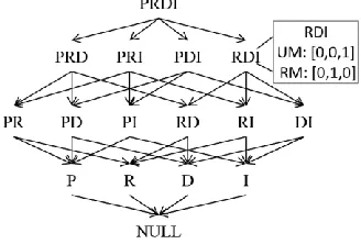
Our proposed lattice (Figure 1), the federated cube lattice, is similar to Harinarayan et al.'s data cube lattice [11] and Bauer and Lehner's distributed aggregation lattice [17]. Our notation operates on a single, integrated lattice with fact tables mapped into a lone, virtual entity F, allowing for JOINs to be performed between nodes.

Figure 1: Example federated cube lattice with RDI expanded to show unrestricted/restricted materialization. Patients (P), Procedures (R),

Diseases (D), and Insurance (I).

The federated cube lattice is a directed acyclic graph (DAG) G whose nodes represent views V (or queries) with edges E corresponding to partial orderings between the views. That is, if there is a path from view u to a view v, then queries on v can also be answered or updated by u. This relationship can be seen from top-down with larger, more generalized views (e.g., u) higher up in the lattice and smaller, more specific views (e.g., v) further down. To model multiple nodes N each cuboid contains a binary vector of size |Nv| – the

number of nodes on which view v resides. This diverges for the distributed aggregation lattice as each view/node pair is a cuboid, which increases the cost of traversing the lattice. To support (un)restricted materialization, a secondary binary vector of size |Nv| is added. The following constraint is

International Journal of Emerging Technology and Advanced Engineering

145 As shown in Figure 1, the structure is similar to that of a standard cube lattice. RDI is expanded to illustrate the two binary vectors (unrestricted (UM) and restricted (RM) materialization) which, in this example, indicates RDI can be materialized on N1, N2, and N3 and is selected for unrestricted materialization on N3 and restricted on N2.

1) View Properties: Each view v ∈ V on node n∈ Nhas an associated query frequency f_vn, update frequency g_vn, reading

cost r_vn (the number of tuples in v on n) Boolean vector _v of size |N| representing unrestricted storage nodes for v, and cost of building from the base relations ς_vB

n = Σb∈vBnϱb where vBn

is the set of base relations required to construct v residing on node n and ϱb = min∀j ≠ n(ψ(b, n), ψ(b, n, j)), which is the

minimum between reading locally and externally (see Section III.B.2) – this is the initial cost of v.

Query frequency is computed from the query set Q as each n has a specific request frequency for v. This view may in fact be the result of a JOIN and/or UNION operation over a set of nodes. For example, n might request RDI with frequency 0.01. RDI may be the result of RD1⋈DI2, thus, both fRD₁ and fDI₂

are updated. Therefore, f_vn = Σq∈Qn _v fqwhere Q n

v⊆Q is the set

of queries containing v on n and fq is the query frequency.

Furthermore, our implementation allows a single view to be answered or updated by a JOIN and/or UNION operation across nodes. Thus, a view is composed of at least one local view, but may be assembled by as many as |N| - 1 additional views. For this to hold, we assume each portion of the materialized view on n is fully computed and stored without an intra-node JOIN and/or UNION. Let the local view be defined by ℓv and the set of external views as εv such that ℓv⨄u ∈ _εv u = v where ⨄∈ {⋈, ∪}.

2) Computing Inter-Node JOINs and UNIONs: The JOIN estimation function proceeds in a linear fashion. If v can be answered fully or in part by the querying node i, then Equation 1 is utilized. This equation first computes the cost of accessing the local portion ℓv_i of vi and sums that with any external fees

from one or more JOINs/UNIONs. If i does not contain a portion of v, then Equation 2 is employed. Initially, the function passes a request for information to node j containing v or the smallest fragment of v. As put forth in Section III.A, the cost of such a request is fixed at one cij. From node j,

Equation 1 is applied sending the results (ψ(vj, j)∂), back to i

upon completion (ψ(vj, j)

∂

(aj + cji)).

The external JOIN cost (Equation 3) applies to any calling node, not just the originating query node and is computed as follows. First, the partial solution to J (initialized to r_ℓv

iai) must

be passed.

This is accomplished by accessing (ai) and transmitting (cij)

the minimum (denoted ∂) amount of information (r∂_J) required.

Those results are then joined with εv (ϕ(r ∂

J, εv)aj) and a

minimum result set returned (ϕ(r∂_J, εv)∂(aj + cji)) to i – ϕ(J, X)

is an estimate of the number of tuples required to perform the JOIN operation(s), and follows Hylock and Currim’s [13] definition.

The cost of a UNION is simply reading and passing the external view εv from j to i – Equation 3. A situation may exist

where both operations are performed to construct a view (e.g., RDI = (RD1∪ RD2) ⋈ DI3).









vi i

vi

i i v

j N

v i r a J i j



  



 













 



      (2)

 





















, , ,

, ,

v

i ij v j v j ji

v j ji J i j

r a c r a r a c if JOIN

a c if UNION

 

   





  



 _{   }



 _



J J J (3)

C. FVSP Formal Definition

Given a federated network H, a mapped fact table F, a relational data warehouse schema Rn ∈ R containing a set of

dimensions Dn ⊆ D, maximum storage space sn, maximum

update cost un, access times an, and a workload of queries Qn

⊆Q for each node n ∈ N, select a set of views M ⊆ V such that

n N MnMto materialize whose combined size is at most sn, combined update cost is at most un, each view v∈Mn is

selected for either restricted or unrestricted materialization, and each external view εv for v∈Mn satisfies v.

1) Federated Cost Model: Our cost model is a reformulation of the Bauer and Lehner extended linear cost model [17]. We broaden this definition to include base relations and account for (un)restricted materialization. Thus, the cost of answering a query requested from node i corresponding to a view v is:

 

 





























, ,

min , , , , , , , , , ,

min , , , , ,

i j Bi

i j Bi

i j v

j i

v j i

q v i

v i v i j v i v i j if v M

v i v i j if v M

 

 

    

  

 

 



 _

 

 

M

(4)

If v∈M, the query cost is the minimum of the local time ψ(vi, i), the external time ψ(vj, i, j), the smallest local

materialized ancestor ψ(vυ, i), the smallest external

materialized ancestor ψ(v_υj, i, j), and base relations ς_vB

i.

International Journal of Emerging Technology and Advanced Engineering

146 The cost of updating a materialized view is equal to the number of changes in the view(s) updating v. Thus, if the changes (Δv) are known, the cost of updating v ∉ M on i corresponds to Equation 5; otherwise a complete reconstruction is performed as described by Equation 6. To the best of our knowledge, this is the first formulation of partial update times in a multi-node environment.







 











, ,

min Δ , , Δ , , , Δ , , ,Δ 0

i j j vBi

j i

u v i

v i v i j v i j if v M

if v M

               M (5)





  











min , , , , , , , , 0

i j j vBi

j i

u v i

v i v i j v i j if v M

if v M

               M (6)

If v∈M, the update cost is the minimum of the local update time ψ(v_υi, i), copying the view from another node updated by

an ancestor or base relations ψ(vυ_j, i, j), the external update time ψ(v_υj, i, j), or the base relations ς_vB

i – Δv follows suit. If v

∉M, no cost is incurred.

2) FVSP Mathematical Model: The suggested model for the FVSP (Equation 7) extends the base MMVSP model. As shown by Hylock and Currim [13], the MMVSP significantly reduces update times with little, if any, effect on query performance. In a federated environment where updates may be generated from outside local networks, update time is of even greater importance; hence, our use of the MMVSP over other extent models.

The FVSP incorporates multiple nodes with the goal of minimizing, over all nodes, the total query and update costs subject to space, update, unrestricted storage, and non-intersecting materialization strategy constraints. As mentioned in Section II.B, the DVSP seeks to minimize the central point of origin. In a federated setting, one must consider every node as a potential entry site and try to account for this accordingly. Therefore, the FVSP seeks to minimize the global cost associated with all nodes.













 

, 0,1 ,

vn vn

n N v Vn v Mn

v_n n v M n

vn n

v M n

v_mn n

m N v

n n

v_n v_n

Minimize f q v M n g u v M n

Subject to r s n N

g u v M n u n N

true n N v M

M M n N

f g v V n N

                                    

 









IV. FEDERATED CUBE LATTICE SEARCH METHODOLOGIES The Federated Cube Lattice can be searched in one or two phases. The singular (extended) approach begins with a full node, UM, and RM solution vector of size 2|N||V| (|Nτ|) resulting in 2|Nτ| possible solutions. It may appear logical to proceed in this manner, but the unrestricted storage vector _v and non-intersecting materialization strategy constraints results in many invalid solutions. We term these the validity constraints (the third and fourth constraints in Equation 7) and say a solution is invalid if violated. As the size of the solution space increases, the number of valid solutions decreases, making initial solution generation and subsequent manipulation more challenging (discussed in Section VII.C). Therefore, we propose a two-phase method (non-extended), that first processes the lattice of views (i.e., without nodes and (un)restricted materialization) identically to the VSP, then allocates those feasible solutions to nodes and materialization strategies. As each view does not fall under the purview of either validity constraint in the initial phase, a solution is guaranteed to hold at the restricted level on their respective node. The benefit here is the ease in constructing initial, feasible solutions using traditional VSP techniques.

The non-extended lattice method requires additional global variables. Each view is assigned a rv and ς_vB value representing

the number of tuples in the final view and the cost of constructing v from the base relations respectively. The query and update frequencies are set to the sum over the network. Finally, the space and update time parameters are θsΣn∈N sn =

Sθand θuΣn∈N un = Uθ where θs, θu∈ [0, 1] designate the

percentage to fill with static views. The greater the values, the less space and update time one has to improve the solution in subsequent iterations.

V. FVSPADAPTED HEURISTICS

International Journal of Emerging Technology and Advanced Engineering

147 A. Modified Heuristics

To convert from the base algorithms to the extended search lattice, |V| increased to |Vτ| and the edge set E expanded to

include all inter-node linkages Eτ. The first phase in a

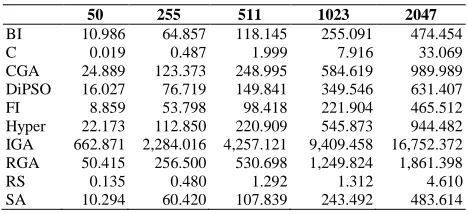
non-extended search is identical to the algorithm's VSP counterpart. The feasible solution Φ found by phase one initializes phase two. For each view in the solution VΦ, at least one valid node and materialization strategy is selected, ensuring the solution remains intact. Table I presents the updated runtimes for RS, FI, BI, SA, RGA, and IGA – C and CGA require additional scrutiny and are saved for the next section. Variables yet to be defined: k is the number of attempts to locate a feasible solution per iteration, N is the number of neighborhoods, n is the number of neighbors, and ρ is the size of the population to generate.

TABLEI

ALGORITHMIC RUNTIMES FOR EXISTING HEURISTICS FOR EXTENDED AND NON-EXTENDED SEARCH –DETAILS IN HYLOCK AND CURRIM [13]

Extended Non-extended

RS O(|Vτ||Eτ|) O(|V||E| + |N||VΦ||Eτ|) FI,BI,SA O(k2

Nn|Vτ||Eτ|) O(k2Nn(|V||E| + |N||VΦ||Eτ|)) RGA O(ρ(ρ + k)|Vτ||Eτ|) O(ρ(ρ + k)(|V||E| + |N||VΦ||Eτ|)) IGA O((ρ2 + k2Nn)|Vτ||Eτ|) O((ρ2 + k2Nn)(|V||E| + |N||VΦ||Eτ|))

1) Constructor and CGA: In addition to the process described in the preceding section, the solution space for the constructor-based heuristic must be further refined. Per the validity constraints, many positions, and therefore combinations, within the search space are invalid. Thus, the heuristic prunes the |Vτ| solution vector to only valid

selections denoted by ϒ, which equals the full complement of terms in the worst case – in general, as |V| and |N| increase, |ϒ| ≪ |Vτ|. This results in an extended runtime of O(ρ(ρ +

k)|ϒ||Eτ|) and non-extended of O(ρ(ρ + k)(|V||E| +

|ϒΦ||Eτ|)), where the valid set for NVΦ is ϒΦ. Combining C with GA produces an extended runtime of O(ρ(ρ + k)|Vτ||Eτ|)

and non-extended of O(ρ(ρ + k)(|V||E| + |N||VΦ||Eτ|)) – note,

these runtimes are equivalent to RGA.

2) Discrete Particle Swarm Optimization: Several modifications to the base DiPSO are necessary to conform to the FVSP solution space. First, initializing the position of each particle x0_i,d (the dth dimension of the ith particle) randomly resulted in too few valid solutions. Thus, a selection rate σ was added to minimize the number of initial views selected for materialization (see Section VII.C for tuning). Per Eberhart et al. [41], a particle’s velocity is limited (clamped) to ±4. Finally, being a discrete problem, the range for x is bound to

{0, 1}, thus the maximum x value for each dimension (xmax)

is 1.

Algorithms 1-3 depict the DiPSO in various stages. Each calls CalculateDiPSO (line 10 of Algorithm 1, 14 of Algorithm 2, and 6 of Algorithm 3), which traverses the federated cube lattice to determine feasibility and validity per Equation 7. The runtime for this method is O(|Vτ||Eτ|). The

result is an extended search runtime of O(ιρk|Vτ||Eτ|) where ι

is the number of iterations, ρ is the number of particles, and k is the number of attempts to locate a feasible solution per iteration.

Phase one of non-extended requires O(ιρk|V||E|) time. The feasible solution set Φ is the input to phase two. If |Φ| > ρ, the top ρ solutions are taken, otherwise ρ = |Φ|. In the worst case, the number of views in Φ (|VΦ|) equals |V|. That is, it is possible to have fewer views in Φ due to the validity constraints, but not necessarily so. Thus, the non-extended runtime is O(ιρk (|V||E| + |N||VΦ||Eτ|)).

Algorithm 1 depicts DiPSO’s initial particle construction process for the extended and phase one of the non-extended search methodologies. Once constructed, line 19 calls the iterative mechanism (Algorithm 3). For the extended search type, Algorithm 3 returns the global best solution. For non-extended, it returns a set of top solutions as seeds for phase two. The second phase is rendered in Algorithm 2 and is virtually identical in operation to Algorithm 1, with the exception of lines 6-13. These lines ensure every selected view has at least one representative in the generated solution.

Algorithm 1: DiPSO

input: particles ρ, iterations ι, inertia weight w, inertia weight degradation α, clamping weight c, attempts k, acceleration coefficients υ1 and υ2, the

max x-value xmax, selection rate σ, and dimensions Vτ

output:gt+1 _{// return global best value}

1. P∅ // population 2. vmax := cxmax // set vmax

3. it := 0 // termination iterator for N

4. for i := 1,…, ρdo // randomly construct initial population 5. if if > kρ set null solution, reset it, and exit end if

6. for d∈ Vτdo

7. v0i,d := U(-vmax, vmax) // random velocity

8. x0i,d := (U(0, 1) > σ ? 1 : 0) // random position

9. end for

10. ifCalculateDiPSO(x) is feasible then

11. P∪ pi // add particle pi to the population

12. _{ˆ :}0 0 i i

x x // set local best 13. if fx0_i < fg0then g0 := x

0

i end if // update global best

14. else 15. i := i - 1 16. end if 17. it := it + 1 18. end for

International Journal of Emerging Technology and Advanced Engineering

148 Algorithm 2: DiPSO-Sub

input: solutions Φ, iterations ι, inertia weight w, inertia weight degradation α, clamping weight c, attempts k, acceleration coefficients υ1

and υ2, the max x-value xmax, selection rate σ

output: gt+1 _{// return global best value}

1. P∅ // population 2. vmax := cxmax // set vmax

3. it := 0 // termination iterator for N 4. for i := 1,…,|Φ| do // construct the extended population 5. ifit > k|Φ|set null solution, reset it, and exit end if

6. for v ∈VΦ_i do // at least one selection for each view

7. r := U(1, |N|) // random number of nodes 8. for j := 1,…,rdo

9. d := U(1, |Nunassigned|) // randomly materialize v on d

10. v0i,d := U(-vmax, vmax) // random velocity

11. if U(0, 1) ≤ 0.5 thenx0i,d := 1 elsex

0

i,d+|N| := 1 end if // UM/RM

12. end for 13. end for

14. ifCalculateDiPSO(x) is feasible then

15. P∪ pi // add particle pi to the population

16. _{ˆ :}0 0 i i

x x // set local best 17. if fx0_i < fg0then g0 := x

0

i end if // update global best

18. else 19. i := i - 1 20. end if 21. it := it + 1 22. end for

23. for i := 1,…, ιdo iterate(P, v, x, w, α, υ1, υ2) end for

Algorithm 3: Iterate

input: particles P, velocity vector v, position vector x, inertia weight w, inertia weight degradation α, acceleration coefficients υ1 and υ2, and

dimensions Vτ

output: (extended or phase two) ? gt+1 _{: g // return best or population}

1. for i ∈Pdo // iterate over the population 2. for d ∈Vτ do

// τ is a random number between 0 and 1 3. 1

, : , 1 , ˆ, , 2 , ,

t t t t t t t

i d i d i d i d i d i d d i d

v w v  _x x _  _g x _// velocity 4.









1

1 _,

,

1 / 1 exp 1

: 0

t

t _{d i d}

i d

otherwis

f v

x

e

i  

 _{ }   

 // discrete position 5. end for

6. ifCalculateDiPSO(i) is feasible then 7. if extended or phase two then // update local and global best values 8. if t1 _ˆt

i i

x x

f  f then xˆ :it1 xti1

 _ 

else _ˆ 1 _ˆ :

t t

i i

x x end if // local 9. if t1 t

i

x g

f  f then

1 1

:

t t

i

g x else 1

:

t t

g g end if // global 10. else

11. if t1 t i

x g

f  f then

1

: t

i

g g x. end if // add to population 12. end if

13. end if 14. end for

15. t := t + 1 // increment time variable 16. wt+1 _{:= αw}t _{// update weight}

3) Hyper-Heuristic: Following Loureiro and Belo [19], the implemented hyper-heuristic utilizes the order SA  DiPSO  RGA. The runtime is therefore a linear combination of its constituent elements, proportional to their utilization.

VI. EXPERIMENTAL SETUP

A five-node federation was configured with |V| ∈ {50, 255, 511, 1023, 2047}. Query and update frequencies were randomly generated. The heuristics were written in Java 7 and executed on a 64-bit Windows 7 machine with an Intel i7-2720QM 2.20GHz processor and 8GB of memory.

VII. COMPUTATIONAL RESULTS

The results are discussed in three parts. The first two compare the heuristics in terms of execution time and objective function value. Lastly, empirical evidence supporting the continued use of the non-extended search methodology is presented. Each experiment was executed ten times with the following exceptions: Hyper and IGA for |V| ≥ 1023 are performed three times due to their run times.

A. Average Execution Time

Tables II and III present the cumulative execution times in seconds per algorithm segmented by dataset size and search lattice methodology. Both RS and C require the least amount of time by a considerable margin. The majority of the heuristics scale fairly evenly at the same magnitude with a few exceptions. IGA performed quite poorly, attributable to the kNn cycles per GA iteration.

TABLEII

EXTENDED LATTICE SEARCH TIMES IN SECONDS

50 255 511 1023 2047

International Journal of Emerging Technology and Advanced Engineering

149 TABLEIII

NON-EXTENDED LATTICE SEARCH TIMES IN SECONDS

50 255 511 1023 2047

BI 10.986 64.857 118.145 255.091 474.454 C 0.019 0.487 1.999 7.916 33.069 CGA 24.889 123.373 248.995 584.619 989.989 DiPSO 16.027 76.719 149.841 349.546 631.407 FI 8.859 53.798 98.418 221.904 465.512 Hyper 22.173 112.850 220.909 545.873 944.482 IGA 662.871 2,284.016 4,257.121 9,409.458 16,752.372 RGA 50.415 256.500 530.698 1,249.824 1,861.398 RS 0.135 0.480 1.292 1.312 4.610 SA 10.294 60.420 107.839 243.492 483.614 There is no significant difference between the two distributions, as neither clearly requires more time. In terms of lattice search, by using a fixed number of iterations, the non-extended approach is virtually guaranteed to work longer; a statement supported by the results. There were a few lower times in the non-extended results, most by an insignificant margin, but IGA for |V| ≥ 511 reported a substantive difference. This is attributable to the decrease in initial invalid and infeasible solutions generated.

B. Average Objective Function Values

Tables IV and V present the average objective function values by algorithm, size, and search methodology – bolded are lowest followed by underlined. Beginning with extended, CGA reported the lowest value for 255-1023, with IGA and DiPSO producing the best solution for 50 and 2047 respectively. The poorest heuristics are RS, SA, FI, and C. Shifting to non-extended, CGA wins across the board. The second best solutions are surprisingly spread out. Hyper turned in the next best performance for 511 and 2047, IGA for 50, SA for 255, and FI for 1023. In terms of poor performers, RS is definitely the leader followed by SA, BI, and C. However, the distance between the best and worst solutions is narrower than with extended.

An inter-search type comparison shows non-extended solutions had lower objective function values 72% of the time, with an average 6.13% improvement.

TABLEIV

EXTENDED LATTICE OBJECT FUNCTION VALUES – IN MILLIONS

50 255 511 1023 2047

BI 47.44 1,545.49 7,935.92 137,191.64 2,050,541,.44 C 48.94 1,592.55 7,972.53 104,954.33 1,308,135.47 CGA 43.70 1,514.23 7,916.91 99,345.48 1,301,718.19 DiPSO 44.26 1,527.31 7,928.57 99,354.14 1,301,373.45 FI 47.56 1,539.53 7,938.23 137,191.64 2,050,541.44 Hyper 44.01 1,536.60 15,672.53 137,191.64 2,050,541.44 IGA 41.29 1,525.32 7,928.05 137,191.64 2,050,541.44 RGA 42.92 1,524.71 7,928.79 99,347.52 1,301,375.31 RS 64.37 2,171.16 10,441.57 221,406.48 6,314,174.05 SA 47.66 1,544.22 7,949.48 99,683.65 1,302,178.90

TABLEV

NON-EXTENDED LATTICE OBJECT FUNCTION VALUES – IN MILLIONS

50 255 511 1023 2047

BI 44.16 1,520.05 7,923.36 100,348.75 1,302,373.40 C 47.45 1,587.06 7,983.06 103,397.13 1,306,882.62 CGA 41.65 1,510.31 7,897.76 99,338.12 1,301,373.20 DiPSO 42.98 1,527.29 7,925.08 99,356.44 1,301,373.33 FI 44.79 1,521.79 7,925.34 99,341.72 1,301,374.62 Hyper 45.15 1,529.51 7,921.95 99,344.05 1,301,373.32 IGA 42.32 1,537.52 7,939.17 99,356.44 1,301,373.49 RGA 42.48 1,532.37 7,932.75 99,523.23 1,311,835.58 RS 66.14 3,178.01 10,319.58 175,955.11 5,869,970.60 SA 45.70 1,513.91 7,948.81 106,933.47 1,302,194.67

C. Generating Valid Solutions

As mentioned several times throughout this section, generating a valid solution appears to be quite difficult especially on the extended search lattice as |Vτ| increases.

Here, evidence is provided to support this claim.

For each experimental input set, the number of valid

positions was determined by materializing all

 

1

V _possible

solutions. As these results in Table VI indicate, the number of valid combinations is quite low compared to the total possible, asymptotically approaching zero. For example, let |V| = 50 and |N| = 5. For each n ∈ N, there are 2 possibilities ((un)restricted materialization) for a total of (50)(5)(2) = 500 elements and 2500 = 3.27×10150 combinations. Only 148 of the possible elements are valid for selection due to the various storage policies, resulting in 3.57×1044 allowable combinations, constricting the solution space to 1.09×10-104% of its original size.

TABLEVI

VALID SOLUTION COMBINATIONS BY LATTICE SIZE

Total Views Valid Elements % Valid

50 500 148 1.09×10-104

255 2,550 845 5.54×10-512

511 5,110 1,785 1.19×10-999

1023 10,230 3,439 5.07×10-2043

2047 20,470 7,686 1.12×10-3792

This effect is also felt when trying to set the section rate σ for DiPSO. Tables VII and VIII present the parameter tuning results for σ ∈ {0.001, 0.01, 0.1, 0.15, 0.2} for 10 attempts at 100 iterations. For the extended approach, it is evident in Table VII that the greater the number of allowable selections from within the |Vτ| solution vector, the more difficult it is to

International Journal of Emerging Technology and Advanced Engineering

150 This is not an artifact of the problem, but a direct result of the two-phase process where every solution in phase one is valid in the restricted case because only views, and not nodes, are selected. Based on these results, σ was set to 0.001.

TABLEVII

AVERAGE NUMBER OF ITERATIONS TO FIND 10FEASIBLE SOLUTIONS IN AN EXTENDED SEARCH

50 255 511 1023 2047

0.001 16 39 237 840 X

0.01 250 X X X X

0.1 X X X X X

0.15 X X X X X

0.20 X X X X X

TABLEVIII

VALID SOLUTION COMBINATIONS BY LATTICE SIZE

50 255 511 1023 2047

0.001 10 10 10 10 10

0.01 10 10 10 10 10

0.1 10 10 10 10 10

0.15 10 10 10 10 10

0.2 10 10 10 10 10

Turning the discussion of feasible solutions back to the experiments performed, we present the total number of empty materialized sets returned by each heuristic in Tables IX and X. Only those with an empty result are shown. The values in bold indicate a complete set of empty results, meaning only the default empty set was materialized for each of their iterations – recall, Hyper and IGA at |V| ≥ 1023 had three runs due to their execution times.

Beginning with the extended search lattice, it is clear as |V| increases the number of returned empty sets follows suit. In fact, for |V| ≥ 511 Hyper did not return a single feasible result, which holds for BI, FI and IGA when |V| ≥ 1023. Interestingly, only DiPSO does not have an II component and all II-based heuristics are listed (recall Hyper incorporates SA). This is attributable to II’s random neighborhood generation function, which does not take into consideration a potentially constrained solution space.

Moving to non-extended, only the II-based heuristics cannot locate a feasible solution for an entire iteration. However, there are clearly fewer empty sets.

TABLEIX

EXTENDED –NUMBER OF EMPTY MATERIALIZED SETS RETURNED

50 255 511 1023 2047

BI 1 7 7 10 10

DiPSO - - - 1 1

FI 2 9 9 10 10

Hyper - 9 10 3 3

IGA - - - 3 3

SA 3 8 9 9 9

TABLEX

NON-EXTENDED –NUMBER OF EMPTY MATERIALIZED SETS

RETURNED

50 255 511 1023 2047

BI - - - 1 1

FI - 1 1 1 2

Hyper - 1 - - 1

IGA - 2 1 1 1

SA - 2 2 3 -

D. Discussion

Combining the results from Section VII.A through VII.C the following heuristic assessments are deduced. CGA and DiPSO are the best overall performing heuristics. Their solutions are amongst the lowest and their execution times and scaling, while not the best, are adequate – neither show a propensity to return an abundance of empty solutions. FI and BI both provide solid objective function values and scale well in terms of time, but as implemented, neither are consistent in finding feasible solutions as |V| increases. IGA also produces objective function values that are quite low, but it does not scale well in terms of time and lattice size. Additionally, although the average execution time for the non-extended search lattice approach is greater than that of extended's (as anticipated due to its two-phase scheme), it is clear the non-extended variant not only finds more feasible solutions during search, but better overall solutions.

VIII. CONCLUSIONS

This paper introduces the federated view selection problem and its constituent components. Prior research in view materialization has been limited to single or distributed configurations, disallowing federated environments. The submitted FVSP consists of five contributions.

International Journal of Emerging Technology and Advanced Engineering

151 Empirical results indicate CGA and DiPSO for the non-extended search lattice consistently provide high quality solutions. The proposed non-extended search approach produces superior results as it pre-satisfies the validity constraints in phase one to provide high quality seeds for the second. These constraints, as depicted, radically reduce the feasible solution space in the traditional, extended search, leading to poorer, if any, solutions.

REFERENCES

[1] M. Banek, A. Tjoa, and N. Stolba. Integrating Different Grain Levels in a Medical Data Warehouse Federation. Data Warehousing and Knowledge Discovery, 2006, pp. 185–194.

[2] S. Berger and M. Schrefl. From Federated Databases to a Federated Data Warehouse System. Proceedings of the 41st Annual HICSS, 2008, pp. 394–403.

[3] L. Kerschberg. Knowledge Management in Heterogeneous Data Warehouse Environments. Data Warehousing and Knowledge Discovery, 2114, 2001, pp. 1–10.

[4] H.-U. Prokosch and T. Ganslandt. Perspectives for Medical Informatics. Methods Inf. Med., 2009.

[5] N. Stolba, M. Banek, and A. M. Tjoa. The security issue of federated data warehouses in the area of evidence-based medicine. The First International Conference on Availability, Reliability and Security, 2006. [6] United States Congress, ―Health Insurance Portability and Accountability

Act,‖ Public Law 104-191, 21-August-1996. http://aspe.hhs.gov/admnsimp/pl104191.htm.

[7] R. Elmasri and S. Navathe. Fundamentals of Database Systems, 5th ed. Addison Wesley, 2007.

[8] H. Garcia-Molina, J. D. Ullman, and J. D. Widom. Database Systems: The Complete Book, Prentice Hall, 2001.

[9] R. Kimball and M. Ross. The Data Warehouse Toolkit: The Complete Guide to Dimensional Modeling, 2nd ed. Wiley, 2002.

[10] J. D. Ullman and J. Widom. A First Course in Database Systems, 3rd ed. Pearson, Prentice Hall, 2008.

[11] V. Harinarayan, A. Rajaraman, and J. D. Ullman. Implementing data cubes efficiently. Proceedings of the ACM SIGMOD. 1996, pp. 205– 216.

[12] R. N. Jogekar and A. Mohod. Design and Implementation of Algorithms for Materialized View Selection and Maintenance in Data Warehousing Environment. Int. J. Emerg. Technol. Adv. Eng., 3(9), pp. 464–470, 2013.

[13] R. Hylock and F. Currim. A maintenance centric approach to the view selection problem. Inf. Syst., 38(7), pp. 971–987, 2013.

[14] R. Chirkova, A. Y. Halevy, and D. Suciu. A formal perspective on the view selection problem. VLDB J., 11(3), pp. 216–237, 2002.

[15] H. Gupta and I. S. Mumick. Selection of Views to Materialize in a Data Warehouse. IEEE TKDE., 17(1), pp. 24–43, 2005.

[16] H. Gupta and I. S. Mumick. Selection of Views to Materialize Under a Maintenance Cost Constraint. International Conference on Database Theory, 1999, 1540, pp. 453–470.

[17] A. Bauer and W. Lehner. On solving the view selection problem in distributed data warehouse architectures. 15th International Conference on Scientific and Statistical Database Management, 2003, pp. 43–51.

[18] L. W. F. Chaves, E. Buchmann, F. Hueske, and K. Böhm. Towards materialized view selection for distributed databases. Proceedings of the 12th International Conference on Extending Database Technology: Advances in Database Technology, 2009, pp. 1088–1099.

[19] J. Loureiro and O. Belo. The M-OLAP cube selection problem: a hyper-polymorphic algorithm approach. Proceedings of the 11th international conference on Intelligent data engineering and automated learning, 2010, pp. 194–201.

[20] J. Loureiro and O. Belo. A Metamorphosis Algorithm for the Optimization of a Multi-node OLAP System. Progress in Artificial Intelligence, 4874, 2007, pp. 383–394.

[21] C. Zhang and J. Yang. Genetic Algorithm for Materialized View Selection in Data Warehouse Environments. Proceedings of the First International Conference on Data Warehousing and Knowledge Discovery, 1999, pp. 116–125.

[22] C. Zhang, X. Yao, and J. Yang. An Evolutionary Approach to Materialized Views Selection in a Data Warehouse Environment IEEE Trans Syst Man Cybern, 31, pp. 282–294, 2001.

[23] T. V. V. Kumar and S. Kumar. Materialized View Selection Using Genetic Algorithm. Contemporary Computing, 2012, pp. 225–237. [24] J. Holland. Adaptation in Natural and Artificial Systems. University of

Michigan Press, 1975.

[25] L. Zhou, X. He, and K. Li. An Improved Approach for Materialized View Selection Based on Genetic Algorithm. J. Comput., 7(7), 2012. [26] D. Yu, W. Dou, Z. Zhu, and J. Wang. Materialized View Selection Based

on Adaptive Genetic Algorithm and Its Implementation with Apache Hive. Int. J. Comput. Intell. Syst., 8(6), pp. 1091–1102,2015.

[27] P. Kalnis, N. Mamoulis, and D. Papadias. View selection using randomized search. DKE, 42(1), pp. 89–111, 2002.

[28] J. Phuboon-ob and R. Auepanwiriyakul. Selecting Materialized Views Using Two-Phase Optimization with Multiple View Processing Plan. World Academy of Science, Engineering and Technology 27, 2007. [29] S. Kirkpatrick, C. D. Gelatt, and M. P. Vecchi. Optimization by

Simulated Annealing. Science, 220(4598), pp. 671–680, 1983.

[30] R. Derakhshan, F. Dehne, O. Korn, and B. Stantic. Simulated annealing for materialized view selection in data warehousing environment. Proceedings of the 24th IASTED international conference on Database and applications, 2006, pp. 89–94.

[31] T. V. V. Kumar and S. Kumar. Materialized View Selection Using Iterative Improvement. Advances in Computing and Information Technology, 2013, pp. 205–213.

[32] T. V. V. Kumar and S. Kumar. Materialized View Selection Using Simulated Annealing. Big Data Analytics, 2012, pp. 168–179.

[33] T. V. V. Kumar and S. Kumar. Materialised view selection using randomised algorithms. Int. J. Bus. Inf. Syst., 19(2), pp. 224, 2015. [34] J. Loureiro and O. Belo. Genetic and Swarm Algorithms for the Selection

of OLAP Data Cubes. Proceedings of the ISCOCO, 2005.

[35] J. Loureiro and O. Belo. A Discrete Particle Swarm Algorithm for OLAP Data Cube Selection. Proceedings of the Eighth International Conference on Enterprise Information Systems, 2006, pp. 46–62.

[36] J. Kennedy and R. C. Eberhart. A discrete binary version of the particle swarm algorithm. IEEE International Conference on Systems, Man, and Cybernetics. 1997, 5, pp. 4104–4108.

International Journal of Emerging Technology and Advanced Engineering

152

[38] P. Cowling, G. Kendall, and E. Soubeiga. A Hyperheuristic Approach to Scheduling a Sales Summit. Practice and Theory of Automated Timetabling III, 2079, 2000, pp. 176–190.

[39] A. Boukra and S. Bouroubi. Selection of views to materialize in data warehouse: A cooperative approach. Stud. Inform. Universalis, 9(2), pp. 19–37, 2001.

[40] F. Glover and C. McMillan. The general employee scheduling problem. An integration of MS and AI. Comput. Oper. Res., 13(5), pp. 563–573, 1986.