ABSTRACT
TAN, QIANWEN. Two-step Methods for Differential Equation Models. (Under the direc-tion of Subhashis Ghoshal.)
In engineering, physics, biomedical sciences, pharmacokinetics and pharmacodynam-ics (PKPD) and many other fields the regression function is often specified as solution of a system of ordinary differential equations (ODEs) given by
dfθ(t)
dt =F(t,fθ(t),θ), t∈[0,1]
here F is a known appropriately smooth vector valued function. Our interest lies in estimating θ from the noisy data.
A two-step approach to solve this problem consists of the first step fitting the data nonparametrically, and the second step estimating the parameter by minimizing the distance between the nonparametrically estimated derivative and the derivative suggested by the system of ODEs. In Chapter 2 we consider a Bayesian analog of the two step approach by putting a finite random series prior on the regression function using B-spline basis. By allowing the parameters to be subject-specific, we further make inference on fixed-effect parameters which characterize how elements of subject-specific parameters vary among individuals due to systematic association with individual attributes.
re-gression driven by a system of ODEs. We study the asymptotic properties of the two-step method estimator based on quantile regression of θ and establish the n−1/2 convergence rate. In Chapter 4 we further explore the Bayesian method for nonparametric quantile regression. We first estimate the whole quantile functions nonparametrically; then for a given τ-level quantile, we apply the two-step approach to estimate the paramter θ
©Copyright 2017 by Qianwen Tan
Two-step Methods for Differential Equation Models
by Qianwen Tan
A dissertation submitted to the Graduate Faculty of North Carolina State University
in partial fulfillment of the requirements for the Degree of
Doctor of Philosophy
Statistics
Raleigh, North Carolina
2017
APPROVED BY:
Anastasios Tsiatis Wenbin Lu
Charles Smith Subhashis Ghoshal
DEDICATION
BIOGRAPHY
ACKNOWLEDGEMENTS
I would like to express my gratitude to my advisor Dr. Subhashis Ghoshal. He provided me great guidance, motivation and encouragement throughout the years on interesting research topics. Without his expertise and illuminating guidance, I could not complete the research work. Besides research, he set a great example to us with his dedication to work, self-motivation, time management skills and perfect balance of life and work. I could not have imagined having a better advisor and mentor for my Ph.D. study.
I wish to thank my committee members, Dr. Anastasios Tsiatis, Dr. Charles Smith, Dr. Wenbin Lu, and Dr. Tao Pang for taking precious time to review my dissertation and share their helpful comments and suggestions to my research.
I am also grateful to all faculty members in the department, who offered a variety of interesting and useful lectures. I also want to thank all the staff members in the department, who provide a friendly and comfortable environment.
Special thanks to all my good friends who shared laughs and tears with me in all these five years.
TABLE OF CONTENTS
LIST OF TABLES . . . vii
LIST OF FIGURES . . . viii
LIST OF SYMBOLS . . . x
Chapter 1 Introduction . . . 1
1.1 Literature review . . . 2
1.1.1 Non-linear least squares approach . . . 4
1.1.2 Two-step approach . . . 4
1.1.3 Bayesian estimation techniques . . . 5
1.1.4 Quantile regression . . . 6
Chapter 2 Two-step Bayesian inference for differential equation models on longitudinal data . . . 9
2.1 Introduction . . . 9
2.2 Model assumptions and prior specifications . . . 14
2.3 Main results . . . 18
2.4 Simulation study . . . 20
2.4.1 Theophylline . . . 20
2.4.2 Bergman’s minimal model . . . 23
2.5 Real data Analysis . . . 25
2.6 Proofs . . . 28
Chapter 3 Two-step approach for quantile regression driven by differ-ential equations . . . 33
3.1 Introduction . . . 33
3.2 Model assumptions . . . 35
3.3 Main results . . . 37
3.4 Simulation study . . . 43
3.4.1 Gamma Data . . . 44
3.4.2 Weibull Data . . . 46
3.5 Real life data . . . 48
3.6 Proofs of theorems . . . 50
3.7 Lemmas and proofs . . . 60
Chapter 4 Two-step approach for nonparametric simultaneous quantile regression driven by differential equations . . . 68
4.2 Model assumptions and prior specifications . . . 69
4.3 Block Metropolis-Hastings MCMC algorithm . . . 72
4.4 Simulation study . . . 74
4.5 Real data analysis . . . 77
LIST OF TABLES
Table 2.1 Coverage and average length of the Bayesian credible intervals using two-step method and confidence interval obtained from nonlinear mixed effects model for Gaussian error for one-compartment model of Theo-phylline. . . 22 Table 2.2 Coverage and average length of the Bayesian credible intervals using the
two-step method and confidence interval obtained from Varah-Brunel method for Gaussian error for Bergman’s minimal model. . . 29 Table 2.3 Coverage and average length of the Bayesian credible intervals using the
two-step method and confidence interval obtained from Varah-Brunel method for the scaled t6 error for Bergman’s minimal model. . . 30 Table 3.1 Monte Carlo bias and MSE of the two-step approach estimators for
quantile regression and mean regression when gamma data with chosen shape function for Lotka-Volterra equations are considered. . . 65 Table 3.2 Monte Carlo bias and MSE of the two-step approach estimators for
quantile regression and mean regression when gamma data with chosen scale function for Lotka-Volterra equations are considered. . . 66 Table 3.3 Monte Carlo bias and MSE of the two-step approach estimators for
quantile regression and mean regression when Weibull data with chosen shape function for Lotka-Volterra equations are considered. . . 67
LIST OF FIGURES
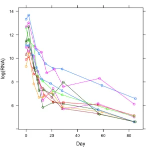
Figure 1.1 Viral load profiles for 10 subjects from the ACTG 315 study. . . 3
Figure 2.1 Theophylline concentrations for 12 subjects following a single oral dose. 11 Figure 2.2 Glucose and Insulin concentrations repeatedly measured over 75
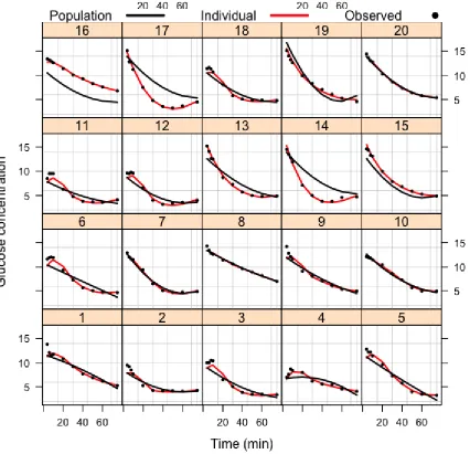
min-utes for 20 healthy individuals in a regular intravenous glucose toler-ance test (IVGTT). . . 13 Figure 2.3 Observed data and individual posterior predictive profiles of glucose
concentration Gθk and population predictive profiles of glucose con-centration Gγ. . . 31
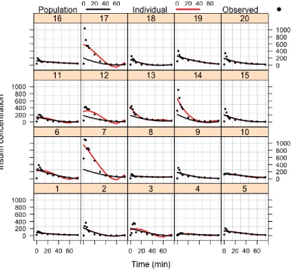
Figure 2.4 Observed data and individual posterior predictive profiles of insulin concentration Iθk and population predictive profiles of insulin concen-tration Iγ. . . 32
Figure 3.1 True derivative of loss function ρand the approximated ψn function. 40
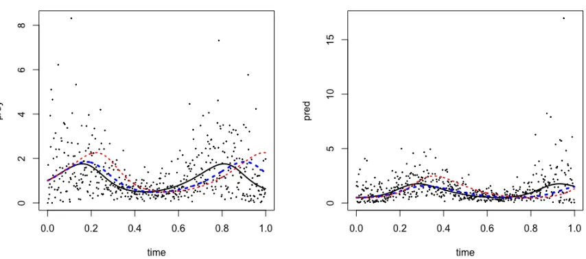
Figure 3.2 Simulation results for gamma data with chosen shape function α(t) = 10t(1−t) + 0.5. The solid black curve is the true quantile function, the dashed blue curve is the estimated quantile function recovered based on two-step quantile regression estimator and the dashed red curve is the estimated quantile function recovered based on two-step mean regression estimator. . . 45 Figure 3.3 Simulation results of gamma data with chosen scale function α(t) =
10t(1−t) + 0.5. The solid black curve is the true quantile function, the dashed blue curve is the estimated quantile function recovered based on two-step quantile regression estimator and the dashed red curve is the estimated quantile function recovered based on two-step mean regression estimator. . . 47 Figure 3.4 Simulation results of Weibull data with chosen shape function α(t) =
1.6t(1−t) + 0.8. The solid black curve is the true quantile function, the dashed blue curve is the estimated quantile function recovered based on two-step quantile regression estimator and the dashed red curve is the estimated quantile function recovered based on two-step mean regression estimator. . . 48 Figure 3.5 Observed values and the predictive profiles of fθ,1 and fθ,2 over the 10
Figure 4.1 Simulation study results for prey population: (a) True quantiles (b) Es-timated quantiles using nonparametric simultaneous quantile regres-sion method at τ = {0.05,0.1,0.2,0.3,0.4,0.5,0.6,0.7,0.8,0.9,0.95} for n = 500 with the data points generated from gamma distribution. 80 Figure 4.2 Simulation study results for predator population: (a) True quantiles (b)
Estimated quantiles using nonparametric simultaneous quantile regres-sion method at τ = {0.05,0.1,0.2,0.3,0.4,0.5,0.6,0.7,0.8,0.9,0.95} for n = 500 with the data points generated from gamma distribution. 81 Figure 4.3 Simulation study results: given τ = 0.5, true quantile function,
LIST OF SYMBOLS
((Aij)) : a matrix Awith (i, j)-th element being Ai,j. AT : transpose of the matrix A.
Ai,: the i-th row of the matrix A. A,j: the j-th column of the matrix A.
rowss
r(A) : the sub-matrix of Aconsisting of r-th to s-th rows of Awith r < s.
colssr(A) : the sub-matrix of Aconsisting of r-th tos-th columns ofA with r < s.
xr:s: the sub-vector consisting of r-th to s-th elements of a vector x.
vec(A) : the vector obtained by stacking the columns of Aone over another.
Ip: the identity matrix of order p.
diag(A1, . . . ,Ap) : block diagonal matrix in which the diagonal elements are square
ma-trices of any size (possibly even 1×1), and the off-diagonal elements are 0. maxeig(A) : the maximum eigenvalue of A.
mineig(A) : the minimum eigenvalue of A. ∥x∥: (∑pi=1xi2)1/2, the L2 norm of the vector x. f′(t) : dtdf(t), the derivative of the function f(·). f(r)(t) : dr
dtf(t), the r-th derivative of the function f(·). f(·) : a vector valued function.
∥f∥w: (
∫1
0 ∥f(t)∥
2w(t)dt)1/2 for a vector valued functionf : [0,1]→Rp andw: [0,1]→
[0,∞).
f(x) : (f(x1), . . . , f(xp))T for a real-valued functionf : [0,1]→R and a vectorx∈Rp.
⟨·,·⟩: inner product.
1A(·) : indicator function of the set A.
an=o(bn) : an/bn→0 as n → ∞for numerical sequences an and bn.
an≍bn: an =O(bn) and bn =O(an).
an≲bn: an =O(bn).
an≪bn: an =o(bn).
oP(1) : a sequence of random variables which converges in probability to zero.
OP(1) : a sequence of random variables bounded in probabiliry.
E(·) the mean vector of a random vector.
Chapter 1
Introduction
Differential equations are encountered in various branches of science such as environmen-tal system, viral dynamics of infectious disease and pharmacokinetics and pharmacody-namics (PKPD). One popular example is the Lotka-Volterra equations, also known as prey-predator equations. At time t ∈ [0,1] the prey and predator populations change according to the equations
dfθ,1(t)
dt = θ1fθ,1(t)−θ2fθ,1(t)fθ,2(t), dfθ,2(t)
dt = −θ3fθ,2(t) +θ4fθ,1(t)fθ,2(t),
where θ = (θ1, θ2, θ3, θ4)T and fθ,1 and fθ,2 denote the prey and predator populations at time t respectively. Another interesting example is HIV dynamics. A set of ordinary differential equations that describes the interaction between HIV virus and human body cells is given by
dX
dt = (1−ϵ)kV T −δX, dV
which has been proven useful for understanding the pathogenesis of HIV infection and de-veloping treatment strategies. In this HIV dynamics model,X andT are size of infected and uninfected immune cell populations, V is the size of the viral population. The pa-rameters in HIV dynamics model is viral clearance ratec, infected cell death rateδ, viral production rate p, probability of infectionk, and treatment efficacyϵ. These parameters characterize intra-subject mechanisms related to interaction between virus and immune system. Note that only the viral load V(t) of the system of ODEs has been measured. Figure 1.1 shows viral load-time profiles for 10 participants in AIDS Clinical Trial Group (ACTG) protocol 315 [49] following initiation of potent antoretrovial therapy. Charac-terizing mechanisms of virus-immune system interaction that leads to such patterns of viral decay (and eventual rebound for many subjects) enhances understanding of the progression of HIV disease.
These models can be put in a regression model, either mean regression or quantile regression model with mean function orτ-th quantile function denoted byfθ : [0,1]→Rd
and fθ satisfies ODE
dfθ(t)
dt =F(t,fθ(t),θ), t∈[0,1], (1.1) here F is a known appropriately smooth vector valued function and θ is a parameter vector controlling the regression function.
1.1
Literature review
1.1.1
Non-linear least squares approach
If the ODEs can be solved analytically, then the usual nonlinear least squares (NLS) technique [29, 31] can be used to estimate the unknown parameters. Thus
ˆ
θ= argmin
θ∈Θ
n
∑
i=1
∥Yi−fθ(xi)∥2,
in many contexts, such closed form solutions are not available as evidenced in some of the previous examples. NLS was modified for this purpose by Brad [1] and Domselaar and Hemker [15]. Hairer et al. [24] and Mattheij and Molenaar [32] used the 4-stage Runge-Kutta algorithm as an alternative approach. The statistical properties of the cor-responding estimator have been studied by Xue et al. [52]. The strong consistency, √ n-consistency and asymptotic normality of the estimator were established in their work.
1.1.2
Two-step approach
Varah [47] used an approach of two-step procedure. In the first step each of the state variables is approximated by a cubic spline using the least squares technique. Let us denote the approximation by ˆf(·). In the second step, the parameter is estimated as
ˆ
θ = argmin
θ∈Θ
n
∑
i=1
fˆ′(t
i)−F(ti,fˆ(ti),θ)
2 .
of the squared deviation, that is
ˆ
θ = argmin
θ∈Θ
∫ 1 0
fˆ′(t)−F(t,fˆ(t),θ)2w(t)dt
and proved √n-consistency as well as asymptotic normality of ˆθ. The order of the B-spline basis is determined by the smoothness ofF(·,·,·) with respect to its first two argu-ments. Gugushvili and Klaassen [22] used the same approach but used kernel smoothing instead of spline. They also established √n-consistency of the estimator. Another mod-ification has been made in the work of Wu et al. [50]. They used penalized smoothing spline in the first step and numerical derivatives instead of actual derivatives of the non-parametrically estimated functions. In another work Brunel et al. [7] used nonparametric approximation of the true solution to (1.1) and then used a set of orthogonality condi-tions to estimate the parameters. The √n-consistency as well as asymptotic normality of the estimator were also established in their work.
1.1.3
Bayesian estimation techniques
ODE models in the Bayesian framework were considered in the works of Gelman et al. [19], Rogers et al. [40] and Girolami [21]. They obtained an approximate likelihood by solving the ODEs numerically. Using the prior assigned on parameters, MCMC technique was used to generate samples from the posterior. This method may suffer from computational complexity as well.
Campbell and Steele [9] proposed the smooth function tempering approach which is a population MCMC technique and it utilizes the generalized profiling approach [36] and the parallel tempering algorithm.
Gaussian process prior on the solution of the ODE and its derivative. The posterior distribution of the solution is used to draw the posterior sample of the parameter of interest. This method is computationally expensive and the likelihood is required to be known for this approach. The theoretical aspects of Bayesian estimation methods have not been yet explored in the literature.
Bhaumik and Ghosal [3] considered the Bayesian analog of the two-step method sug-gested by Brunel [6], putting a prior on the coefficients of the B-spline basis functions and induced a posterior on parameter space. Bhaumik and Ghosal [3] further developed an efficient two-step method Bayesian estiamation by directly considering the distance between the function in the nonparametric model and that obtained from RK4 method. They established a Bernstein-von Mises theorem for the posterior distribution of param-eters with n−1/2 contraction rate.
1.1.4
Quantile regression
Yu and Moyeed [55] first introduced the quantile regression using Bayesian methods. Later Kottas and Gelfand [27], Gelfand and Kottas [18], Geraci Bottai [20] and Kottas and Krnjajic [28] proposed a few methods on generalization and extension of single level quantile regression under different possible scenarios.
The main disadvantage of considering separate quantile regression using single level quantile regression is that the natural ordering among different quantiles can not be en-sured. Addressing the non-crossing issue, He [25] proposed a quantile regression method assuming the response variable to be heteroskedastic. Neocleous and Portnoy [33] pro-posed a method to estimate the quantile curve using linear interpolation from an esti-mated gird of quantile curves. Takeuchi [43] and Takeuchi et al [44] proposed non-crossing quantile regression methods using support vector machine (SVM) [46]. Later Shim et al. [42] used doubly penalized kernel machine (DPKM) for estimating non-crossing quantile curves.
Dunson and Taylor [16] and Liu and Wu [30] proposed quantile regression methods for a grid of quantiles addressing the monotonicity constraint. Later Wu and Liu [51], Reich [37], Reich et al. [38], Reich and Smith [39] proposed linear quantile regression methods addressing the non-crossing issues. Recently, Tokdar and Kadane [45] and Das and Ghosal [13] proposed simultaneous linear quantile regression methods for univariate explanatory variables. Yang and Tokdar [53] extended that simultaneous linear quantile regression method to handle multivariate predictor case.
Chapter 2
Two-step Bayesian inference for
differential equation models on
longitudinal data
2.1
Introduction
oral dose D(mg/kg) of the anti-asthmatic agent theophylline, and blood samples drawn at several times following administration were assayed for theophylline concentration. As ordinarily observed in this context, the concentration profiles have a similar shape for all subjects; however peak concentration achieved, rise and decay vary substantially. These differences are believed to be attributable to inter-subject variation in the un-derlying pharmacokinetic process, understanding which is critical for developing dosing guidelines. To characterize these processes formally, it is a routine practice to represent the body by a simple compartment model [41]. For theophylline, the pharmacokinetics is modeled using a one-compartment model shown in (2.1) with first order absorption and elimination
dfθ,1(t)
dt =−kafθ,1(t), dfθ,2(t)
dt =kafθ,1(t)−kefθ,2(t),
(2.1)
where the initial status are fθ,1(0) =D and fθ,2(0) = 0. There are two differential
equa-tions in the one-compartment model. Since it is only theophylline serum concentration C(t) which is measured, we do not have measurements for compartment 1 while that of compartment 2, C(t) is equal to fθ,2(t) divided by the serum volume V = Cl/ke. The parameters in the one-compartment model are the first-order absorption rateka, the
first-order elimination rateke, and the clearance rateCl. For theophylline, a one-compartment
model is standard and has solution of the corresponding differential equations which yields
C(t) = Dkake Cl(ka−ke)
{
exp(−ket)−exp(−kat)
}
. (2.2)
disap-Figure 2.1: Theophylline concentrations for 12 subjects following a single oral dose.
muscles, liver and tissue is raised by the remote insulin in action. This lowers the glu-cose concentration in plasma, implying the β-cells to secrete less insulin, from which a feedback effect arises. This integrated glucose-insulin system can be described by the following non-linearly coupled system of differential equations [17]
dG(t)
dt =−p1(G(t)−Gb)−X(t)G(t), G(0) =G0, dX(t)
dt =−p2X(t) +p3(I(t)−Ib), X(0) = 0, dI(t)
dt =−p4(I(t)−Ib) +p5(G(t)−p6)t, I(0) =I0,
(2.3)
where t = 0 is the glucose injection time. Diabetes is associated with a large number of abnormalities in insulin metabolism, ranging from an absolute deficiency to a combination of deficiency and resistance, causing inability to dispose glucose from the blood stream. Three factors, referred to as the metabolic portrait [34] and playing important roles for glucose disposal, are glucose effectiveness SG = p1, insulin sensitivity SI = p3/p2, and pancreatic responsiveness ϕ1 =
Imax−Ib
p4(G0−Gb)
and ϕ2 =p5×104.
Figure 2.2: Glucose and Insulin concentrations repeatedly measured over 75 minutes for 20 healthy individuals in a regular intravenous glucose tolerance test (IVGTT).
individuals are needed so that estimation of the subject-specific parametersθk is feasible and the large sample approximation to the distribution of ˆθk may be applied. In this
chapter, we consider the case when number of repeated measurements n is suficiently large to support fitting the individual model separately by individual to obtain reason-able subject-specific estimators for θk. In the first stage, we consider the individual-level
model. For each individual k, 1 ≤ k ≤ l, we carried out a Bayesian analog of two-step appoach of Brunel [6] fitting a nonparametric regression model using the B-spline basis. We assign priors on the coefficients of the basis function. A posterior is then induced on
θk using the posterior of the coefficients of the basis functions. In the second stage, we
consider a population model that we fit the subject-specific parameters θk by individual
parameters and individual characteristics.
The chapter is organized as follows. Section 2.2 contains the model assumptions and prior specifications. The main results are given in Section 2.3. In Section 2.4 we carry out simulation studies under different settings. We analyze a real life data in Section 2.5. Proofs of the main theorems are given in Section 2.6.
2.2
Model assumptions and prior specifications
We have a system of d ordinary differential equations (ODEs) given by
dfθ,j(t)
dt =Fj(t,fθ(t),θ), t∈[0,1], j = 1, . . . , d, (2.4)
where fθ(·) = (fθ,1(·), . . . , fθ,d(·))T and θ ∈ Θ, a compact subset of Rp. Let us denote F(·,·,·) = (F1(·,·,·), . . . , Fd(·,·,·))T. We also assume that for a fixed θ, F ∈ Cm−1((0,
1),Rd) for some integerm >1. Then, by successive differentiation of the right hand side of (2.4), it follows that fθ ∈Cm((0,1)). By the implied uniform continuity, the function and its several derivatives uniquely extend to continuous functions on [0,1].
For each individual, we consider an n×d matrix of observations ofYk for 1≤k ≤l
with Yij denoting the measurement taken on the j-th response at the time point ti,
0 ≤ ti ≤ 1, i = 1, . . . , n and j = 1, . . . , d. For the k-th individual, denoting εk =
((εijk))1≤i≤n,1≤j≤d as the corresponding error matrix. The proposed model is given by
while the data is generated by the model
Yijk =fk,j0 (ti) +εijk, i= 1, . . . , n, j = 1, . . . , d, k = 1, . . . , d,
where fk0(·) = (fk,01(·), . . . , fk,d0 (·))T denotes the true mean vector for the k-th individual which does not necessarily belong to the {fθ : θ ∈ Θ}. We also denote the true mean
matrix by f0 = ((f0
k,j))1≤k≤l,1≤j≤d. We assume that f0 ∈Cm([0,1]). Let εijk iid
∼P0, which is a probability distribution with mean zero and finite varianceσ2
0 fori= 1, . . . , n,j = 1, . . . , dand k= 1, . . . , l.
In the first stage we consider the individual-level model focusing on the subject-specific parameter θk for k = 1, . . . , l. Since the expression for fθ is usually not available, the
proposed model is embedded in the nonparametric regression model fork-th individual
Yk =XnBn,k+εk, (2.5)
where Xn = ((Ns(ti)))1≤i≤n,1≤s≤Jn, {Ns(·)}
Jn
s=1 being the B-spline basis functions with orderm and kn−1 interior knots with increasing dimension Jn =kn+m−1. We choose
interior knots 0< ξ1 < ξ2 <· · ·< ξkn−1 <1 to satify the pseudo-uniformity criterion:
max
1≤i≤kn−1|ξi+1−2ξi+ξi+1|=o(k −1
n ),
max 1≤i≤kn−1|
ξi−ξi−1|
min
1≤i≤kn−1|ξi−ξi−1| ≤M,
(2.6)
for some constant M. Here ξ0 and ξkn are defined as 0 and 1 respectively. The criterion (2.6) is required to apply the asymptotic results obtained in Zhou et al. [56] where they mention the similar criterion in equation (3) of that paper. Here we denoteBn,k =
(
βJn×1
. . . ,βJn×1
k,d
)
the matrix containing the coefficients of the basis functions for d responses. We considerP0 to be unknown and useN(0, σk2) as the working distribution for the error
of the k-th individual where σk should be treated as another set of unknown parameters
for k = 1, . . . , l. Denoting by Qn, the empirical distribution funtion of ti, i = 1, . . . , n,
we assume that for some probability measure Q on [0,1] with positive and continuous density
sup
t∈[0,1]
|Qn(t)−Q(t)|=o(kn−1). (2.7)
For each individual k, we put an inverse gamma prior on σ2
k which is given by
σk2 ∼InvGamma(a0k, b0k).
Conditional on σ2
k, let the prior distribution on the coefficients be given by
βk,j|σ2k∼ N
(
0, n2kn−1σk2IJn
)
.
Simple calculation yields the posterior distribution for βk,j as
βk,j|(Yk),j ∼ N
((
XnTXn+
knIJn n2
)−1
XnT(Yk),j, σk2
(
XnTXn+
knIJn n2
)−1)
(2.8)
and the posterior distributions of βk,j and βk,j′ are mutually independent for j ̸= j′; j, j′ = 1, . . . , d. In the model of (2.5), the expected response vector at a point t ∈[0,1] is given by BT
n,kN(t), where N(·) = (N1(·), . . . , NJn(·))
T.
(0,1). We define
Rf(η) =
{ ∫ 1 0
∥f′(t)−F(t,f(t),η)∥2w(t)dt
}1/2
ψ(f) = argmin
η∈Θ
Rf(η).
It is easy to check that ψ(fη) =η for all η∈Θ. Thus the map ψextends the definition
of the parameter θk beyond the model. Let us define θ0,k = ψ(fk0). Thus θ0,k describes
the projection of the true regression function on the parametric model. We assume that
θ0,k lies in the interior of Θ. A posterior of θk is induced on Θthrough the mapping ψ
acting on f(·) =BT
n,kN(·) and the posterior of Bn,k given by (2.8).
Remark 2.1. Note thatf0(·) need not be a solution of the ODE. In real life it is almost impossible to accurately describe a data generating mechanism in terms of a mathemati-cal model. ODE is a useful tool to model many dynamic systems within a margin of error. This justifies the study of misspecified regression function in the context of ODE model. Often we are more interested in inferring on the parameters rather than the regression function described by the ODE model. Then the role of the true parameter is played by the parameter value which brings the ODE model closest to the true regression function. The definition of θ0 reinforces this intuition.
At the second stage, we consider the population-level model
θk =d(xk,γ,ηk) (2.9)
where d is a p-dimensional function depending on an r ×1 vector of fixed effects γ,
ηk is a p×1 vector of random effects associated with individual k, and xk is vector
θk vary among individuals, due to systematic association with individual attributes in xk and to unexplained variations in the population of individuals, for example, natural,
biological variation, represented by ηk. Sometimes we are interested in certain function h(·) of θk instead of θk itself. In this case, population model can be easily modified to
be h(θk) = d(xk,γ,ηk). A common special case of (2.9) is that of a linear relationship
between θk and fixed and random effects as in usual, i.e., θk = Xkγ +ηk where Xk is
a design matrix depending on elements of xk. Define θ = (θT1, . . . ,θTl )T and X = (X1T, . . . ,XlT)T to be the design matrix for the fixed effect. Then the second step of two-step procedure is given by the optimization as follows:
argmin
γ,η1,...,ηl
l
∑
k=1
∫ 1 0
∥fβ′k(t)−F(t,fβk(t),Xkγ+ηk)∥2w(t)dt.
Motivated by the linear population model, the induced posterior of fixed effect γ is obtained as (XTX)−1XTθ and the induced posterior of random effects η
k = θk − Xk(XTX)−1XTθ.
2.3
Main results
Our objective is to study the asymptotic behavior of the posterior distribution of√n(γ− γ0). The asymptotic representation of
√
n(γ −γ0) is given by the next theorem under the assumption that for all ϵ > 0, inf
η:∥η−θ0,k∥≥ϵRf 0
k(η) > Rf
0
k(θ0,k) for k = 1, . . . , l. We denote Dl,r,sF(t,f,θ) = ∂l+r+s/∂θs∂fr∂tlF(t,f(t),θ). Let the matrix
Jθ0,k =
∫ 1 0
[
(D0,0,1F(t,fk0(t),θ0,k))TD0,0,1F(t,fk0(t),θ0,k)−D0,0,1Sk(t,fk0(t),θ0,k)
]
be nonsingular, whereSk(t,f(t),θ) = (D0,0,1(F(t,f(t),θ)))T((fk0(t))′−F(t,fk0(t),θ0,k)).
Letm ≥5 and n1/2m ≪k
n≪n1/8. Also define
Γk(z) =
∫ 1 0
([
D0,1,0Sk(t,fk0(t),θ0,k)−(D0,0,1F(t,fk0(t),θ0,k))TD0,1,0F(t,fk0(t),θ0,k)
]
w(t)
−d
dt[(D0,0,1F(t,f 0
k(t),θ0,k))Tw(t)
)
z(t)dt.
LetAk(t) stands for thep×d matrix
Jθ0−1
,k
([
D0,0,1Sk(t,fk0(t),θ0,k)−(D0,0,1F(t,fk0(t),θ0,k))TD0,0,1F(t,fk0(t),θ0,k)
]
w(t)
−d dt
[
(D0,0,1F(t,fk0(t),θ0,k))Tw(t)
])
.
Then we have, with (Ak),j standing for thejth column ofAk(t),
Jθ0−1
,kΓk(fk) =
d
∑
j=1
∫ 1 0
(Ak),j(t)NT(t)βk,jdt= d
∑
j=1
GTk,jβk,j, (2.10)
where GT k,j =
∫1
0(Ak),j(t)N
T(t)dt which is a p×J
n matrix for j = 1, . . . , d and k = 1,
. . . , l.
Theorem 2.1. Define
µk =
√ n
d
∑
j=1
GTk,j(XnTXn)−1XnT(Yk),j−
√ nJθ−1
0,kΓ(f 0
k),
Σk = n d
∑
j=1
Gk,j(XnTXn)−1GTk,j
. . . , l. Define µ= (µT
1, . . . ,µTk)T. Let
µγ = (XTX)−1XTµ,
Σγ = (XTX)−1XT diag(Σ1, . . . ,Σl)X(XTX)−1.
(2.11)
IfHk,jis nonsingular for allj = 1, . . . , d,k = 1, . . . , l, andD0,2,1F(t,y,θ)andD0,0,2F(t,
y,θ)are continuous in their arguments, then on a set in the sample space with high true
probability, then the posterior distribution of √n(γ−γ0) assigns most of its mass inside
a large compact set, which implies that the posterior distribution of γ − γ0 contracts
at 0 at the rate of n−1/2 with high probability under the truth. Moreover, the posterior
distribution of √n(γ−γ0) is approximated by a normal distribution as follows
∥Π(√n(γ−γ0)∈ ·|Y)− N(µγ, σ02Σγ)∥TV =oP0(1). (2.12)
2.4
Simulation study
2.4.1
Theophylline
We consider the one-compartment model shown in (2.1) to study the posterior distri-bution of γ. This set of ODEs describes the pharmacokinetics process of absorption, distribution and elimination governing concentration of drug theophylline achieved. We consider the case that the true regression function is the solution of the ODEs. We are interested in three parameters, the first-order absorption rate ka, the first-order
elimi-nation rate ke and the clearance rate Cl. For the population model, we reparameterize
model is assumed to be given by
k∗a,k=γ1+η1k, k∗e,k =γ2 +η2k, Cl∗k=γ3+η3k
is a linear population model. This model enforces positivity of the pharmacokinetics parameters for each k. Understanding the typical values of the parameters in f, how they vary across individuals in the population, and whether some of this variation is associated with individual characteristics may be addressed through inference on the parameters γ. The components of γ = (γ1, γ2, γ3)T describe both the typical values and the strength of systematic relationships between elements of subject-specific parameters
θk.
We consider l = 12 individuals in the simulation study. For each individual and sample size n, the ti’s are observed time points, which are chosen to be equally-spaced
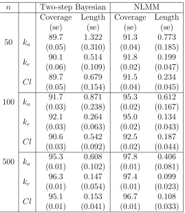
Table 2.1: Coverage and average length of the Bayesian credible intervals using two-step method and confidence interval obtained from nonlinear mixed effects model for Gaussian error for one-compartment model of Theophylline.
n Two-step Bayesian NLMM
Coverage (se) Length (se) Coverage (se) Length (se) 50 ka
89.7 (0.05) 1.322 (0.310) 91.3 (0.04) 0.773 (0.185) ke 90.1 (0.06) 0.514 (0.109) 91.8 (0.02) 0.199 (0.047) Cl 89.7 (0.05) 0.679 (0.154) 91.5 (0.04) 0.234 (0.045) 100 ka
91.7 (0.03) 0.871 (0.238) 95.3 (0.02) 0.612 (0.167) ke 92.1 (0.03) 0.264 (0.063) 95.0 (0.02) 0.134 (0.043) Cl 90.6 (0.03) 0.542 (0.092) 92.5 (0.02) 0.187 (0.044) 500 ka
95.3 (0.01) 0.608 (0.102) 97.8 (0.01) 0.406 (0.081) ke 96.3 (0.01) 0.147 (0.054) 97.4 (0.01) 0.099 (0.023) Cl 95.1 (0.01) 0.153 (0.041) 96.7 (0.01) 0.108 (0.033)
we have p = 3, d = 1 and the ODEs are given by (2.1) for t ∈ [0,25] with initial conditions fθ,1(0) = 4.02 and fθ,2(0) = 0. Then take γ0 = (0.466,−2.455,−3.228)T. We generate the data from Yijk = fθ0,k,j(ti) +εijk, where fθ0,k,j(·) representing the j-th compartment mean function, satisfies the corresponding ordinary differential equation with true subject-specific parameters being θ0,k.
The true distribution of error εijk among the repeated measurements is taken to be
σ2
k, we put Gaussian priors on the coefficients βk|σ2k with mean vector 0 and dispersion
matrixn2k
nσk2IJn for two-step Bayesian method. We choosekn−1 equally-spaced interior knots. As far as choosingkn is concerned, we take m= 3 and kn = 10,15,20 for n = 50,
100 and 500 respectively guided by Theorem 2.1 and cross validation. The simulation results are summarized in the Tables 2.1. Not surprisingly the NLMM based confidence intervals obtained from the NLS method are shorter and with an higher coverage rate. When there is an explicit solution to the ODEs system, we definitely will choose the NLS method over the two-step method. Nevertheless the two-step method gives the coverage even if it is not as efficient as the NLS method when solution is explicit.
2.4.2
Bergman’s minimal model
We consider Bergman’s mininal model of glucose disappearance shown in (2.3) to study the posterior distribution of γ. We consider the case that the true regression function is the solution of the ODE. We are interested in the following three factors, glucose effectiveness SG = p1, insulin sensitivity SI =p3/p2 and pancreatic responsivenessϕ1 =
Imax−Ib
p4(G0−Gb)
and ϕ2 = p5 ×104. Consider these factors as functons h(·) of the original parameters θk. For the population model, a single parameter is associated with each
fixed effect, with independent random effect, i.e. h(θk) = γ +ηk for k = 1, . . . , l. We consider l = 20 individuals in the simulation study. For each individual and sample size n, the ti’s are observed time point, which are chosen to be equally-spaced and spread
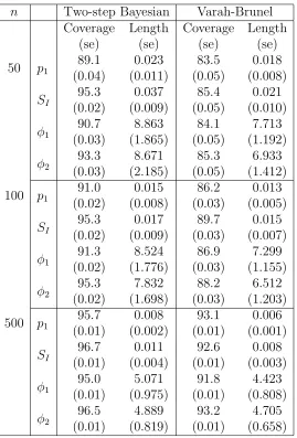
the coverage and the average length of the corresponding credible interval over these 500 replicates. The estimated standard error of the interval length and coverage are given inside the parentheses in the tables. Our method is abbreviated as “Two-step Bayesian” in the tables. We also consider 500 replications to construct the 95% equal tailed confidence interval based on asymptotic normality as obtained from the estimation method introduced by Varah [47] and modified and studied by Brunel [6]. We abbreviated this method as “Varah-Brunel” in the tables. The estimated standard errors of the interval length and coverage are given inside the parentheses in the tables.
In this example, not all states of the system of ODEs have been measured; the remote insulin compartment, represented byX(t) has not been measured. In this case, we replace X(t) by the solution of the differential equation given by
X(t) = p3e−p2t
∫ t
0
ep2sI(s)ds−p3Ibe−p2t
(ep2t−1
p2
)
.
Note that the optimization step for the third compartmentI(t) is linear in the parameters if we reparameterizep∗6 =p5p6. Hence the optimization step is equivalent to obtaining an ordinary least square solution. For the first compartment, after we replace X(t) by the above equation, it is linear in the parameters p1 and p3. We first treat p2 as known and solve for p1 and p3 as functions of p2 which we optimize using standard tools.
differential equation with true subject-specific parameters being θ0,k.
The true distribution of errorεijk in the repeated measurements is taken eitherN(0,
52) or a scaled t-distribution with 6 degrees of freedom, where scaling is done in order to make the standard deviation 5, where i = 1, . . . , n, j = 1, . . . , d and k = 1, . . . , l. We put an inverse gamma prior on σ2
k with shape and scale parameters being 100 and
0.01 respectively. Conditional on σk2, we put Gaussian priors on the coefficients βk,1|σk2
and βk,2|σk2 with mean vector 0 and dispersion matrix n2knσk2IJn for two-step Bayesian method. We choosekn−1 equally-spaced interior knots. We choose m= 6 and kn = 16,
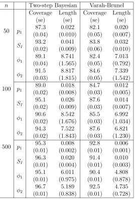
17,20 for n = 50,100 and 500 respectively. The simulation results are summarized in the Tables 2.2 and 2.3. Not surprisingly asymptotic normality based confidence intervals obtained from the “Varah-Brunel” method are shorter but too optimistic, failing to give adequate coverage for finite sample sizes since the delta method is known underestimate variation.
2.5
Real data Analysis
in a 30% solution) is administered intravenously over a 60 seconds period to 20 healthy overnight-fasted subjects, and subsequently the glucose and insulin concentrations in plasma are repeatedly measured at 0, 2, 4, 6, 8, 10, 20, 30, 40, 50, 60 and 75 minutes. The individual glucose and insulin profiles are shown in Figure 2.2. We have two main interests in this real data analysis: (i) recover the true individual profiles of glucose and insulin concentrations using our two-step Bayesian approach; (ii) study the impact of body mass index (BMI) and gender to insulin sensitivity for healthy subjects.
We use B-spline basis of order 7 with kn= 2. We put an inverse gamma prior on σ2
with shape and scale parameters 100 and 0.01 respectively and usew(t) =t0.5(1−t)0.5,t∈ [0,1]. Conditional onσ2
k we put a Gaussian prior onβwith mean vector0and dispersion
matrix n2k
nσ2kIJn. Samples of size 500 are drawn from the posterior distributions of subject-specific parametersθ = (p1, p2, p3, n, γ, h, G0, I0)T. For the population model, we introduce two subject covariates which are body mass index (BMI) as x1 and gender as x2 (x2 = 1 for female andx2 = 0 for male), hence the population model can be written as θk =γ0+γ1x1k+γ2x2k+ηk fork = 1, . . . , l. We recover the individual profiles Gθk(·) and Iθk(·) by using the posterior of subject-specific parameters θk. We set the random effect to be 0 to obtain population profilesGγ(·) andIγ(·). The individual posterior predictive
profiles of Gθk(·) and Iθk(·) are superimposed on the data in Figure 2.3 and 2.4 by solid red curve; and the population posterior predictive profiles of Gγ(·) and Iγ(·) are
12, 13 and 18; as for other subjects, the glucose concentrations decays at a stable rate from 0 minute to 75 minutes, i.e., subject 1, 8, 9, 10 and 16. Also, we note that for subject 14, 16 and 17 the individual profile is quite different from the population profile, it can be interpreted as that the variations among the subject-specific paramters are not fully explained by BMI and gender. There are some unexpained variations remain which are attributible to random effects. This phenomenon is also shown in Figure 2.4 for subject 2, 7, 8, 9 and 17.
IVGTT study.
2.6
Proofs
Proof of Theorem 2.1. Following Bhaumik and Ghosal [2], we know that the posterior
distribution of each subject-specific parameter θk for k = 1, . . . , l,
√
n(θk −θ0,k) is
ap-proximated by a normal distribution with mean vector µk and dispersion matrix σ02Σk.
This distribution matches with the frequentist distribution of the estimator in Brunel [6]. Note thatγ = (XTX)−1XTθ, is a linear function ofθ whereθ = (θT
1, . . . ,θlT)T. So it is
straightforward to state that the posterior distribution of√n(γ−γ0) is approximated by a normal distribution with mean vector µγ and dispersion matrix σ02Σγ given by (2.11).
Since the asymptotic mean µk of the posterior distribution of each θk matches with the centerized and normalized distribution of the estimator in Brunel [6], it follows that
µk is stochastically bounded. Hence µγ is stochastically bounded as the dimension of
design matrix X is pl×r and fixed.
In the proof of Lemma 4 of Bhaumik and Ghosal [2], they have already shown that the eigenvalues of Gk,j(XnTXn)−1Gk,j are of the order of n−1. The eigenvalues of asymptotic
Table 2.2: Coverage and average length of the Bayesian credible intervals using the two-step method and confidence interval obtained from Varah-Brunel method for Gaussian error for Bergman’s minimal model.
n Two-step Bayesian Varah-Brunel
Coverage (se) Length (se) Coverage (se) Length (se)
50 p1 89.1
(0.04) 0.023 (0.011) 83.5 (0.05) 0.018 (0.008) SI 95.3 (0.02) 0.037 (0.009) 85.4 (0.05) 0.021 (0.010) ϕ1 90.7 (0.03) 8.863 (1.865) 84.1 (0.05) 7.713 (1.192) ϕ2 93.3 (0.03) 8.671 (2.185) 85.3 (0.05) 6.933 (1.412) 100 p1
91.0 (0.02) 0.015 (0.008) 86.2 (0.03) 0.013 (0.005) SI 95.3 (0.02) 0.017 (0.009) 89.7 (0.03) 0.015 (0.007) ϕ1 91.3 (0.02) 8.524 (1.776) 86.9 (0.03) 7.299 (1.155) ϕ2 95.3 (0.02) 7.832 (1.698) 88.2 (0.03) 6.512 (1.203) 500 p1
Table 2.3: Coverage and average length of the Bayesian credible intervals using the two-step method and confidence interval obtained from Varah-Brunel method for the scaled t6 error for Bergman’s minimal model.
n Two-step Bayesian Varah-Brunel
Coverage (se) Length (se) Coverage (se) Length (se)
50 p1 87.3
(0.04) 0.022 (0.010) 82.1 (0.05) 0.020 (0.007) SI 93.2 (0.02) 0.041 (0.009) 83.8 (0.06) 0.032 (0.010) ϕ1 89.1 (0.04) 8.741 (1.565) 82.4 (0.05) 7.013 (0.792) ϕ2 91.5 (0.03) 8.817 (1.815) 84.6 (0.05) 7.339 (1.542) 100 p1
89.0 (0.02) 0.018 (0.008) 84.7 (0.03) 0.012 (0.005) SI 95.1 (0.02) 0.026 (0.009) 87.6 (0.03) 0.014 (0.007) ϕ1 90.6 (0.02) 8.542 (1.676) 85.5 (0.03) 6.992 (1.034) ϕ2 94.3 (0.02) 7.522 (1.843) 87.6 (0.03) 6.821 (1.230) 500 p1
Chapter 3
Two-step approach for quantile
regression driven by differential
equations
3.1
Introduction
functions. Koenker and Bassett [26] discussed advantages of quantile regression in some non-Gaussian settings.
In this chapter we consider a two step approach for quantile regression driven by a system of ODEs. For a fixed 0 < τ < 1, let the τth quantile of the response variable Y be denoted by Qτ(Y|t). The ODE model assumes that Qτ(Y|t) is described by a set
of ODEs in t containing a set of unknown parameters. In the two-step approach, we first estimate the quantile function and its derivatives nonparametrically using B-spline basis expansion. We then minimize the distance between the nonparametric estimate of the derivative and that obtained from the ODE with the nonparametric estimate of the quantile function plugged in the equations defining the model. We study the asymp-totic properties of the two-step approach estimator based on quantile regression of θ
error needs to be accounted in the estimates. Secondly, their approach is based on a sufficiently smooth criterion function, but the criterion function for the quantile function is even discontinuous. We therefore modify our approach using a sequence of smooth cri-terion functions approximating the one for the quantile function. Thus two modifications of the results of Yohai and Maronna [54] are needed: allowing a sequence of criterion functions instead of a fixed one and letting the model to be slightly misspecified in that the true distribution does not belong to the model but the approximation error decays to zero sufficiently fast. Both modification requires carefully dealing with the terms arising due to the approximations to the criterion function and the truth.
The chapter is organized as follows. Section 3.2 contains the model assumptions. The main results are given in Section 3.3. In Section 3.4 we carry out simulation studies under different settings. We analyze a real life data in Section 3.5. Proofs of the main theorems are given in Section 3.6 and those of some auxiliary lemmas in Section 3.7.
3.2
Model assumptions
Consider a matrix of observations Y with Yij as entries denoting the ith measurement
taken on thejth response variable at the time point ti where i= 1, . . . , nand j = 1, . . . ,
d. The observations can be represented by Y = ((Yij))1≤i≤n,1≤j≤d = (Y1(n×1), . . . ,Y
n×1
d ).
The unknown quantile function Qτ(Y|t) = (Qτ(Yj|t) : j = 1, . . . , d) of observations of Y as a function oft with a set of unknown parameters θ is denoted by fθ(t) where the
dynamics of the unknown function fθ(t) can be described by the following system of
ordinary differential equations
dfθ(t)
where fθ(·) = (fθ,1(·), . . . , fθ,d(·))T, F(·,·,·) = (F1(·,·,·), . . . , Fd(·,·,·))Tand θ ∈ Θ. We
assume that Θis a compact subset of Rp.
The first step of the two-step approach is to fit the nonparametric quantile regression model at the given quantile levelτ. Here we use B-spline basis functions to fit the quantile regression Qτ(Y|t) =XnBn where Qτ(Y|t) is theτth quantile function of observations Y evaluated at the given time pointst = (t1, . . . , tn)T; Xn = ((Nl(ti)))1≤i≤n,1≤l≤Jn = (x1, . . . ,xn)T ∈Rn×Jn,{Nl(·)}Jl=1n being the B-spline basis functions with order mand kn−1
interior knots with Jn=m+kn−1, andxi being theith row vector of matrix Xn with
increasing dimension Jn for i = 1, . . . , n, and Bn =
(
βJn×1
1 , . . . ,β
Jn×1
d
)
is the matrix containing the coefficients of the basis functions for d responses. The loss function of quantile regression for a given τ using the B-spline basis expansion can be written as
ρ
(Y −XnBn) whereρ(u) =ρτ(u) = τ u−1{u≤0}u.In the first step, we carry out the nonparametric estimation of Qτ(Y|t) using the
B-spline basis expansion. We minimize the loss function
ρ
(Y−XnBn) to obtain the quantileregression coefficient Bnb =
( b
βJ1n×1, . . . ,βbdJn×1
)
. In the second step, we estimate the parameterθby minimizing a weighted distance between the nonparametrically estimated derivative and the derivative suggested by the system of ODEs. Letw(·) be a continuous weight function withw(0) =w(1) = 0 and be positive on (0,1). We define
Rf(η) =
{ ∫ 1 0
∥f′(t)−F(t,f(t),η)∥2w(t)dt
}1/2
ψ(f) = argmin
η∈Θ
Rf(η). (3.2)
It is easy to check that ψ(fη) = η. Thus the map ψ extends the definition of the parameter θ beyond the model. Let us define f0 = (f0,1, . . . , f0,d)T the true quantile
θ0 describes the projection of the true regression function on the parametric model. We assume that θ0 lies in the interior of Θ. From now on, we shall write θ for ψ(f) and treat it as the parameter of interest. The estimator of θ is induced on Θ through the mapping ψ acting on f(·) = BbT
nN(·).
3.3
Main results
Our objective is to study the asymptotic behavior of the two-step method estimator and obtain an asymptotic representation of √n( ˆθ−θ0). We make the assumption that
for all ϵ >0, inf
η:∥η−θ0∥≥ϵRf0(η)> Rf0(θ0). (3.3)
We denote mixed derivatives as Dl,r,sF(t,f,θ) = ∂l+r+s/∂θs∂fr∂tlF(t,f,θ). The
re-sponse variables Yj’s are considered independent, and hence βˆj are mutually
indepen-dent forj = 1, . . . , d. This allows treating regression for each response variable separately. Thus we can assume that d= 1 in Theorem 1 for the sake of simplicity in notation and write ˆf(·), f0(·), F(·,·,·), βˆ instead of fˆ(·), f0(·), F(·,·,·) and Bnb respectively. Exten-sion to d-dimensional case is straightforward as shown in Remark 4 after the statement of Theorem 1.
Remark 3.1. Condition (3.3) implies that θ0 is the unique point of minimum of Rf0(·)
and θ0 should be a well-separated point of minimum.
Theorem 3.1. Let the matrix
Jθ0 =
∫ 1 0
[
(D0,0,1F(t, f0(t),θ0))TD0,0,1F(t, f0(t),θ0)−D0,0,1S(t, f0(t),θ0)
]
be nonsingular, where S(t, f(t),θ) = (D0,0,1(F(t, f(t),θ)))T(f0′(t)−F(t, f0(t),θ0)). Let m ≥ 5 and n1/2m ≪ J
n ≪ n1/8. If D0,2,1F(t, y,θ) and D0,0,2F(t, y,θ) are continuous in
their arguments, then under the assumption (3.3), we have
∥√n(θˆ−θ0)−Jθ0−1
√
n(Γ( ˆf)−Γ(f0))∥ →P0 0 (3.4)
as n → ∞, where
Γ(z) =
∫ 1 0
([
D0,1,0S(t, f0(t),θ0)−(D0,0,1F(t, f0(t),θ0))TD0,1,0F(t, f0(t),θ0)
]
w(t)
−d
dt[(D0,0,1F(t, f0(t),θ0))
Tw(t))z(t)dt.
Remark 3.2. In Lemma 3.3, we show thatΓ( ˆf)−Γ(f0) = Op(n−1/2). Henceθˆconverges θ0 at the rate n−1/2 in probability under the truth.
Remark 3.3. We note that fifth order smoothness of the true mean function is sufficient to ensure that the convergence rate is n−1/2. We do not gain by assuming a higher order of smoothness. For m = 5, the required condition becomes n1/10 ≪ Jn ≪ n1/8. Also,
deterministically chosen equally spaced knots are sufficient to derive the parametric rate.
Remark 3.4. When the response is ad-dimensional vector, (3.4) holds with the scalars being replaced by the correspondingd-dimensional vectors. Let A(t) stands for the p×d matrix
Jθ0−1
([
D0,0,1S(t,f0(t),θ0)−(D0,0,1F(t,f0(t),θ0))TD0,0,1F(t,f0(t),θ0)
]
w(t)
−d dt
[
(D0,0,1F(t,f0(t),θ0))Tw(t)
])
Then we have, with A,j standing for thejth column of A(t),
Jθ0−1Γ(fβ) = d
∑
j=1
∫ 1 0
A,j(t)NT(t)βjdt= d
∑
j=1
GTn,jβj, (3.5)
where GTn,j =∫01A,j(t)NT(t)dt which is ap×Jn matrix for j = 1, . . . , d. Then in order
to approximate the distribution of ˆθ, it suffices to study the asymptotic distribution of the linear combination of ˆβj given by (3.5).
Theorem 3.2. Let τ2
n = EFψn2/(EFψn′)2 and define Σn = n
∑d j=1G
T
n,j(XnTXn)−1Gn,j.
Then under the conditions of Theorem 3.1, √nτ−1
n Σ
−1/2
n ( ˆθ−θ0)converges in distribution
to Np(0,I).
To estimate quantile function Qτ(Y|t) nonparametrically using the B-spline basis
expansion, we estimate the coefficient of quantile regression β of the basis functions by
ˆ
β = argmin
β n
∑
i=1
ρ(Yi−x′iβ) (3.6)
where the loss function is defined as ρ(u) = ρτ(u) = τ u−1{u ≤ 0}u. If ρ were convex
with derivativeψ, then (3.6) would be equivalent to the solution of
n
∑
i=1
ψ(Yi−x′iβ)xi = 0.
technical obstacles. Further, as the B-spline expansion is only an approximation, the truth does not belong to the model and the model is mildly misspecified. Figure 3.1 shows the derivative function and its approximation by a sequence of smooth functions given by
ψn(un) = τ −1 +
(
1 + τ 1−τe
−Snun
)−1
whereSn → ∞. The differentiability ofψn function will be seen to play an important role
in the asymptotic properties of the estimation. This motivates us to define the estimator ˆ
β as any of the solution of
n
∑
i=1
ψn(Yi−x′iβ)xi = 0. (3.7)
According to the property of B-splines there always exist β0 and constantcsuch that
sup
t∈[0,1]
|fβ0(t)−f0(t)|2 ≤cJn−2m, sup t∈[0,1]
|fβ0′ (t)−f0′(t)|2 ≤cJn−2(m−1). (3.8)
Note that for such β0, we could not define β0 to be a solution of
E0(ψn(Y −fβ(t))) = 0
because ψn is not the same as ψ for the chosen τ and fβ0(t) is not the τth quantile ofY
for a given t. Instead, for such β0 satisfying (3.8), we could only have the following such that for some ηn>0,
|E0(ψn(Y −fβ0(t)))| ≤ηn.
Suppose there exist positive sequencesbn,cnanddnsuch thatD(u, z) =
ψn(u+z)−ψn(u)
z ≥