Music Classification using Support Vector Machine Ms. Shabnam R. Makandar

353 | P a g e

Music Classification using Support Vector Machine

Ms. Shabnam R. Makandar

Assistant Professor, MCA Department, D. Y. Patil Institute of MCA, Akurdi, Pune, Maharashtra, (India)

ABSTRACT

Increasing amount of online music content has opened new opportunities for implementing new effectual information access

services commonly known as music recommender systems that support music navigation, discovery, sharing, and formation of

user communities. A music retrieval approach based on various similarity information, integrate multiple feature similarities,

including content-based and context-based similarities such as Timbral Texture Features and Rhythmic Content Features. Audio

classification is very essential for faster retrieval of audio files. Extracting most excellent set of features and deciding top

analysis method is very important for getting best results of audio classification. Support vector machines are applied to classify

music into pure music and vocal music by learning from training data. The sequential minimal optimization (SMO) algorithm has

been generally used for training the support vector machine. For pure music and vocal music, a number of features are extracted

to illustrate the music content, respectively. Based on calculated features, a clustering algorithm is applied to structure the music

content. Finally, a music summary is created based on the clustering results and domain knowledge related to pure and vocal

music. Support vector machine learning shows a better performance in music classification.

Keywords: Classification, Feature Extraction, Feature Selection, MIR, Support Vector Machine.

I. INTRODUCTION

Music Information Retrieval (MIR) is a very narrow specialty within IR, and it needs different approaches than other subjects in the field. Before the growth of the internet and more technologically advanced systems, musical works for the purposes of libraries were organized using alphabetic classified systems[18].

In other words, they were described according to their physical characteristics. Traditionally, systems for bibliographic IR were designed with the physical document in mind [17]. While text-based retrieval of music documents using the composer's name, an opus number, or lyrics can be handled using conventional IR techniques, this text-based approach is not enough for retrieval of music, in all of its forms. Smiraglia makes the case that instead of conceptualizing music as a physical document be it a score or a recording the idea of a musical `work' should be the “key entity" upon which MIR is based [9].

Music classification has received much attention from MIR researchers in recent years. In the MIR community, an annual event Music Information Retrieval Evaluation eXchange1 (MIREX) is held for competitions on important tasks in MIR since 2004. Most of the high-level tasks in MIREX competitions are relevant to music classification. Those tasks directly related to music classification are listed in the following.

354 | P a g e

 Mood Classification

 Artist Identification

 Instrument Recognition

 Music Annotation

There have been a few survey articles in the relevant research field in previous years. Scaringella et al. reviewed the techniques of audio feature extraction and classification for the task of genre classification only. Weihs et al. focused on music classification in general but did not pay much attention to the subtle differences between different tasks, as different types of features may vary in performance for different tasks [5]. Moreover, the field of music classification research is developing fast in the past few years, with new features and types of classifiers being developed and used. More importantly, the task of music annotation has recently achieved much popularity in the MIR community since the work of Turnbull et al. in 2007. The purpose of music annotation is to annotate each piece of song with a set of semantically meaningful text annotations called tags. A tag can be any relevant musical term that describes the genre, mood, instrumentation, and style of the song. Hence, music annotation can be treated as a classification problem in the general sense, where tags are class labels that cover different semantic categories. Music classification can employ a collection of hundreds of low-level features (e.g., zero-crossing rate, MFCCs, LPC coefficients) and higher-order variations on these (e.g., standard deviation, first-order difference). Extracting hundreds of features from a large music collection, however, is costly in terms of both time and space. Moreover, ideally, the size of a classifier's training set should increase exponentially with the number of features [2]. However, it is not necessarily instinctive which of the possible features will be most relevant to a high-level music classification task, such as genre or artist identification, so it is logical to look for an automated way of selecting a good subset of the available features.

The fast development of various modest technologies for multimedia content capturing, data storage, high bandwidth/speed transmission, and the multimedia compression standards such as JPEG and MPEG, have resulted in a rapid increase of the size of digital multimedia data collections and greatly increased the availability of multimedia contents to the general user[12].

355 | P a g e

Figure 1: Audio Classification Hierarchy [12]

II.

LI TERATURE REVIEW

The important components of a classification system are feature extraction and classifier learning. Feature extraction addresses the problem of how to represent the examples to be classified in terms of feature vectors or pairwise similarities. The purpose of classifier learning is to find a mapping from the feature space to the output labels so as to minimize the prediction error.

2.1 Classifiers for Music Classification

This is the setting for the majority of music classification tasks. In standard classification, it is presented with a training data set where each example comes with a label. The objective is to design a classification rule that can perfect predict the labels for unseen data.

Classifier design is a standard topic in pattern classification. The frequent choices of classifiers are K-nearest neighbor (K-NN, support vector machine (SVM), and GMM. Various other classifiers have also been used for different music classification tasks, logistic regression artificial neural networks (ANN), decision trees, linear discriminant analysis (LDA), nearest centroid (NC), and sparse representation- based classifier (SRC).

356 | P a g e

Figure 2: Binary tree for multi-class classification[10].

The use of GMM as a classifier should not be jumbled with its use for modeling the timbre features. In the latter case, GMMs are used for song-level similarity computation. This is dissimilar from classifier learning. For the GMM classifier, fit the Gaussian mixture model over the distributions of song-level features in each class. With the class conditional probability distribution, a testing example can be labeled according to the following Bayes rule.

The decision is based on the maximize of the posterior probability P (x | y)(y specifies the labels, specifies the data). P

(x | y) specifies the conditional probability of example x for class label y valued from the training data using GMM, and P(y) is the prior probability stipulating the proportion of label y in the training data. Specifically, GMM classifier can be used for feature set input, too. By assuming that timbre features in each class are independent and identically distributed, we can relate the product rule to estimate the class conditional probability for feature sets. Another classifier that can directly handle feature set classification is convolutional neural network (CNN), which is a generalization of the standard neural network model by taking complications over the segments of the input signal. Hence, such model can be used for audio classification based on sequence of timbre features like raw MFCC features. This is confirmed with applications on general audio classification using a convolutional deep belief network (CDBN), an extension of CNN with multiple layers of network.

2.2 Feature Learning

357 | P a g e

There is a subtle difference between automatic feature selection and extraction. In the previous case, features are directly selected from a large number of candidate input features based on some feature selection rules. For feature extraction, features are obtained from transformations of the input features based on several feature mapping or projection rule. Feature selection/extraction can be done in either supervised or unsupervised fashion. In the supervised setting, labeled data are used to help the selection or extraction of useful features that best distinguish between different labels. One possible approach for feature selection is to gain knowledge of a front-end classifier like logistic regressor, which can be trained efficiently, and rank the attributes based on the classifier weights. The lowest ranked feature attributes are then discarded in training the final classifier. Alternatively, one can perform linear feature extraction by learning a transformation matrix to project higher dimensional feature vectors to a lower dimensional subspace that preserves most of the discriminate information. This is achieved by a variety of metric learning algorithms found to be useful for feature learning in music classification. An important metric learning method useful for genre classification is linear discriminant analysis (LDA), which finds the optimal transformation by maximizing between -class scatter while minimizing intra-class scatter. Unsupervised feature extraction methods process input features based on modeling the essential structure of the audio signal without making use of the label information. A standard method for unsupervised feature extraction is principal component analysis (PCA), which projects the input features to a lower dimensional space that maximally preserves the covariance. PCA is normally used as the post processing step for decorrelation in the extraction of standard timbre features like OSC. Non-negative matrix factorization (NMF) provides another approach to unsupervised feature extraction, which aims at obtaining a factorization of the matrix of feature vectors into the product of two low rank matrices with non-negative entries. NMF can improve lower dimensional features with non-negative feature values. This is pretty useful for music feature representation and is found to deliver good empirical performance for genre classification. An extension of NMF to tensors, called non-negative tensor factorization (NTF), is also used in music genre classification for input tensor features and has demonstrated the best performance when combined with specific features and classifiers.

2.3Feature Combination and Classifier Fusion

If multiple features are available, we can combine them in some manner for music classification. Feature combination from different sources is an effective way to develop the performance of music classification systems. A straightforward way to feature combination is to concatenate all features into a single feature vector, for combining timbre with beat and pitch features. Feature combination can also be incorporated with classifier learning. Multiple kernels learning (MKL) is one such framework developed particularly for SVM classifiers. The purpose of MKL is to learn an optimal linear combination of features for SVM classification. MKL has recently been applied to music classification and found to do better than any of the single feature types.

358 | P a g e 0

recognized by the technique of stacked generalization (SG), which provides a cascaded framework for classification by stacking classifiers on top of classifiers. In the SG framework, classifiers at the first level are trained on individual features, and classifiers at the second level are trained by using the decision values returned by level-1 classifiers as new features. Hence, SG obtains the fusion rule through supervised learning. The selection of classifiers used for SG is quite flexible. Normally SVMs are used within SG for optimized performance. Different combination strategies have been studied, showing that SG and MKL achieve the best performances for multi-feature music genre classification, outperforming other existing methods by a significant margin. Another important class of feature combination methods is based on group methods for classification. One such example is AdaBoost with decision trees (AdaBoost, DT), which combines decision tree classifiers[5].

III.

MUSIC-SPEECH CLASSIFICATION

Two types of features are computed from each frame for music-speech classification: 1) perceptual features, composed of total power, subband powers, brightness, bandwidth, and pitch and 2) MFCCs. Their definitions are given in the following, where the FFT coefficients F (ω) are computed from the frame.

•

Total Spectrum Power. Its logarithm is used: log( ω0 |F (ω)|2), where |F (ω)|2 is the power at the frequency is the half sampling frequency.

•

Subband Powers. The frequency spectrum is divided into four subbands with intervals.

•

Brightness. The brightness is the frequency centroid.

•

Bandwidth. Bandwidth is the square root of the power-weighted average of the squared difference between the spectral components and the frequency centroid.

•

Frequency. A simple pitch detection algorithm, based on detecting the peak of the normalized autocorrelation function, is used. The pitch frequency is returned if the peak value is above a threshold or the frame is labeled as non-pitched otherwise.

•

Mel-Frequency Cepstral Coefficients: These are computed from the FFT power coefficients. The power coefficients are filtered by a triangular bandpass filter bank.

359 | P a g e

IV. FEATURE SELECTION

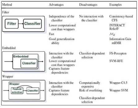
Feature selection, also known as variable selection, attribute selection or variable subset selection, is the process of selecting a subset of relevant features for use in model construction. The central supposition when using a feature selection technique is that the data contains many redundant or irrelevant features. Redundant features are those which give no more information than the currently selected features, and irrelevant features give no useful information in any context. Feature selection techniques are a subset of the more general field of feature extraction. Feature extraction generates new features from functions of the original features, whereas feature selection returns a subset of the features. Feature selection techniques are frequently used in domains where there are many features and comparatively few samples (or data points).

Feature selection aims to choose a subset of features from high-dimensional data according to a predefined selection criterion. It can bring many benefits such as removing irrelevant and redundant features, reducing the chance of overfitting, saving computational cost, improving prediction accuracy, and enhancing result clarity. Many feature selection algorithms have been proposed in the past several years. According to the availability of class label information, feature selection can be categorized as supervised feature selection, unsupervised feature selection, and semisupervised feature selection.

Figure 4: Feature Selection Techniques

4.1 Supervised Feature Selection

360 | P a g e

4.2Unsupervised Feature Selection

For unsupervised feature selection, preserving local geometric structure of data becomes much more important. This is because unsupervised feature selection aims to select the features that can well maintain the fundamental data structure. In this case, preserving the local geometric structure of data will be more useful, especially considering that high-dimensinal data often presents a low-dimensional manifold structure. Unsupervised feature selection chooses features that can effectively disclose or maintain the underlying structure of data.

4.3Semi-Supervised Feature Selection

Semisupervised feature selection, instead, selects a discriminative feature subset by utilizing both labeled and unlabeled data[11].

V. SUPPORT VECTOR MACHINE

In machine learning, support vector machines (SVMs, also support vector networks) are supervised learning models with associated learning algorithms that analyze data and recognize patterns, used for classification and regression analysis. Given a set of training examples, each clear as belonging to one of two categories, an SVM training algorithm builds a model that allots new examples into one category or the other, making it a non- probabilistic binary linear classifier. An SVM model is a representation of the examples as points in space, mapped so that the examples of the separate categories are divided by a clear space that is as large as possible.[14]

SVM is a useful technique for data classification. Even though it’s considered that Neural Networks are easier to

use than this, however, every so often unsatisfactory results are obtained. A classification task usually involves with training and testing data which consist of some data instances. Each example in the training set contains one target values and several attributes. The objective of SVM is to produce a model which predicts target value of data instances in the testing set which are given only the attributes[17].

Classification in SVM is an example of Supervised Learning. Known labels help indicate whether the system is performing in a right way or not. This information points to a most wanted response, validating the correctness of the system, or be used to help the system learn to act correctly. A step in SVM classification involves identification as which are intimately connected to the known classes. This is called feature selection or feature extraction. Feature selection and SVM classification together have a use even when prediction of unknown samples is not essential. They can be used to identify key sets which are involved in no matter what processes distinguish the classes.

361 | P a g e

remaining classes, which is defined as one against- all. An- other approach is to translate a n-class problem into n(n + 1)/2 two-class problems which cover all pairs of classes. This method is called pairwise classification. There is no theoretical analysis of the two strategies with respect to classification performance. However, regarding the training effort, the one-against-all approach is preferable since only n SVMs have to be trained evaluated to n(n+1)/2 SVMs in the pairwise approach.

Figure 5: (a)Feature Extraction and (b)SVM Prediction[14]

Figure 6: SVM method for speech and music discrimination in different training set [10].

362 | P a g e

VI. IMPLEMENTATION DETAILS

Given a set of training vectors belonging to two separate classes, (x1, y 1 )...(xl, yl) where xi∈ Rnand yi∈ {−1, +1}

, one needs to find out the hyperplane wx + b = 0 to divide the data so as to maximizes the margin (the distance between the hyperplane and the nearest data point of each class). The solution to the optimization problem of SVM is given by the saddle point of the Lagrange function.

The SVM can understand nonlinear discrimination by kernel mapping[2]. The samples of non- linear feature in the input space cannot be separated by any linear hyperplanes, but can be linearly separated in the non-linear mapped feature space hyperplanes. The optimal separating hyperplane with the largest margin recognized by the dashed lines, passing the support vectors.[14].

6.1 Sequential Minimal Optimization Algorithm

The SMO algorithm is to solve the controlled quadratic programming problem. It takes the concept of chunking to the great limit and to consider just two Lagrange multipliers at a time. The SMO algorithm searches through the feasible region of the dual problem and maximizes the objective function by choosing two Lagrange multipliers and jointly optimizes them (with all the others fixed) at each iteration.

The SMO Algorithm: initial

w=0,b=0 and all α=0,E=0

loop

choose two Lagrange multiplier and jointly optimize

Calculate prediction error Ei, Ej and αieta, αjeta, gamma.

Determine the feasible range [L,H] for clipping

and Clipping to L or H

αnew = αold + _yiyj (αold − αnew )

update w, b, delta b. update prediction error E.

363 | P a g e

6.2 Comparison of SVM with different classifier

Figure 8: Comparison of accuracy of SVM with other classifiers

Figure 9: Global accuracy comparison using consecutive segments of a song[1].

VII RESULTS

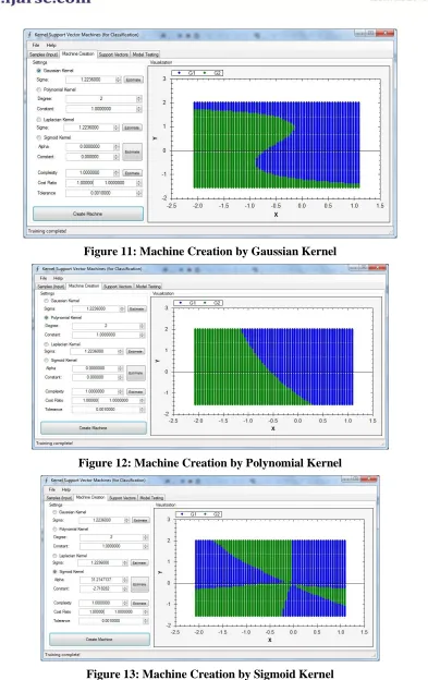
Support Vector Machine Classifier is implemented using Visual Studio 2012 and .Net Framework 4.5 for the audio classification after the feature extraction process. The extracted features are then classified.

364 | P a g e

Figure 11: Machine Creation by Gaussian Kernel

Figure 12: Machine Creation by Polynomial Kernel

365 | P a g e

Figure 14: Support Vector

Figure 15: Model Testing of Support Vector

VIII CONCLUSION

Selection of the most excellent contributing features to be extracted and the selection of the top suited method of classification are the most important decisions to be made for the content based audio classification. SVMs can be trained efficiently for audio classification.

First, a set of training data is available and can be used to train a classifier. Second, once trained, the calculation in a SVM depends on a usually small number of supporting vectors and is speedy. Third, the distribution of audio data in the feature space is complex and different classes may have overlapping or interwoven areas. A kernel based SVM is well right to handle such a situation.

366 | P a g e

exclusive optimal solution for each selection of the SVM parameters. This is different in other learning machines, such as standard Neural Networks trained using back propagation.

In short, the development of SVM is an totally different from normal algorithms used for learning and SVM presents a new insight into this learning. The four most major features of SVM are duality, kernels, convexity and sparseness.

ACKNOWLEDGEMENT

I wish to thank all the people who gave me an unending support. I take this opportunity to convey my sincere thanks to Mrs. V. L. Kolhe for their advice and valuable guidance that helped me in making this paper interesting and successful one. I also thank all those who have directly or indirectly guided and helped. Last but not the least I thank my family, friends and well wishers for their continuous support and boosting confidence in me.

REFERENCES

[1] N. Auguin, Shilei Huang, and P. Fung. Identification of live or studio versions of a song via supervised learning. In Signal and Information Processing Association Annual Summit and Conference (APSIPA), 2013 Asia-Pacific, pages 1–4, Oct 2013.

[2] Lei Chen, S. Gunduz, and M.T. Ozsu. Mixed type audio classification with support vector machine. In Multimedia and Expo, 2006 IEEE International Conference on, pages 781–784, July 2006.

[3] Y.M.G. Costa, L. Oliveira, AL. Koerich, and F. Gouyon. Comparing textural features for music genre classification. In Neural Networks (IJCNN), The 2012 International Joint Conference on, pages 1–6, June 2012.

[4] Zhouyu Fu, Guojun Lu, Kai Ming Ting, and Dengsheng Zhang. Learning naive bayes classifiers for music classification and retrieval. In Pattern Recognition (ICPR), 2010 20th International Conference on, pages 4589–4592, Aug 2010.

[5] Zhouyu Fu, Guojun Lu, Kai Ming Ting, and Dengsheng Zhang. A survey of audio-based music classification and annotation. Multimedia, IEEE Transactions on, 13(2):303–319, April 2011.

[6] V.B. Kobayashi and V.B. Calag. Detection of affective states from speech signals using ensembles of classifiers. In Intelligent Signal Processing Conference 2013 (ISP 2013), IET, pages 1–9, Dec 2013.

[7] G. Kotsalis, A. Megretski, and M.A. Dahleh. A model reduction algorithm for hidden markov models. In Decision and Control, 2006 45th IEEE Conference on, pages 3424–3429, Dec 2006.

[8] Ta-Wen Kuan, Jhing-Fa Wang, Jia-Ching Wang, and Gaung-Hui Gu. Vlsi design of sequential minimal optimization algorithm for svm learning. In Circuits and Systems, 2009. ISCAS 2009. IEEE International Symposium on, pages 2509– 2512, May 2009.

[9] S.Z. Li. Content-based audio classification and retrieval using the nearest feature line method. Speech and Audio Processing, IEEE Transactions on, 8(5):619–625, Sep 2000.

[10]Stan Z. Li Lie Lu and Hong-Jiang Zhang. Content-based audio segmentation using support vector machines.

[11]Xinwang Liu, Lei Wang, Jian Zhang, Jianping Yin, and Huan Liu. Global and local structure preservation for feature selection. Neural Networks and Learning Systems, IEEE Transactions on, 25(6):1083–1095, June 2014.

367 | P a g e

Distributed Framework and Applications (DFmA), 2010 International Conference on, pages 1–6, Aug 2010.

[13]V. Panagiotou and N. Mitianoudis. Pca summarization for audio song identifica- tion using gaussian mixture models. In Digital Signal Processing (DSP), 2013 18th International Conference on, pages 1–6, July 2013.

[14]N.P. Patel and M.S. Patwardhan. Identification of most contributing features for audio classification. In Cloud Ubiquitous Computing Emerging Technologies (CUBE), 2013 International Conference on, pages 219–223, Nov 2013.

[15]S. Scardapane, D. Comminiello, M. Scarpiniti, and A. Uncini. Music classification us- ing extreme learning machines. In Image and Signal Processing and Analysis (ISPA), 2013 8th International Symposium on, pages 377–381, Sept 2013.

[16]Xi Shao, Changsheng Xu, and M.S. Kankanhalli. Unsupervised classification of music genre using hidden markov model. In Multimedia and Expo, 2004. ICME ’04. 2004 IEEE International Conference on, volume 3, pages 2023–2026 Vol.3, June 2004.

[17]A. Tjahyanto, Y.K. Suprapto, M.H. Purnomo, and D.P. Wulandari. Fft-based fea- tures selection for javanese music note and instrument identification using support vector machines. In Computer Science and Automation Engineering (CSAE), 2012 IEEE International Conference on, volume 1, pages 439–443, May 2012.

[18]EnShuo Tsau, S. Chachada, and C.-C.J. Kuo. Content/context-adaptive feature selection for environmental sound recognition. In Signal Information Processing As- sociation Annual Summit and Conference (APSIPA ASC), 2012 Asia-Pacific, pages 1–5, Dec 2012.

[19]G. Tzanetakis and P. Cook. Musical genre classification of audio signals. Speech and Audio Processing, IEEE Transactions on, 10(5):293–302, Jul 2002.