DISTRIBUTIONS OF RANDOM-FIELDS IN SOLIDS - CONTRIBUTION OF THE NEAREST DEFECT

Distributions of random fields in solids: contribution of

the nearest defect

A M Stoneham

Theoretical Physics Division, Building 424.4, AERE, Harwell, Oxon OX11 ORA, UK

Received 26 August 1982

Abstract. This paper discusses the statistical distribution of internal fields due to random defects in solids. It extends previous discussions by separating explicitly the contribution of the nearest defect from that due to all others. Possible applications include those to prefer- ential defect pairing, to hopping conduction in randomly doped crystals, and to questions of

the existence of phase transitions in random dipole systems. As a by-product. we note that the random strains in solids have a statistically negligible probability of localising a muon (assumed not self-trapped) except at the sites of defects themselves.

1. Introduction

There are many cases in which observable effects arise from the random fields of statistically distributed defects in solids. The fields themselves may be strain fields, electric fields, or it may be the electrostatic potential or electrical field gradient which varies from site to site. This subject was reviewed by Stoneham (1969), who surveyed the methods of calculating the distribution I(&) deof an internal field E.

Calculations of the distribution involve two main pieces of information. First, one needs to know the contribution E(z) to E of a single defect whose relative position and other defining parameters are given by

z .

Secondly, one needs to know something about the statistical distribution. This is usually described by a straightforward generalisation

p ( z ) of the pair distribution function of the defects causing the random field relative to the probe species which monitors I(&). Given expressions forp(z), E(Z) and the density of defects one can calculate the distribution I ( & ) . One can also obtain the moments of the distribution M.v, where

M,v

=

i

d &I( E)

c",

and some special features like asymptotic expressions. The moments, however, are rarely useful, since they do not always correspond to what is measured, and often diverge, though they are simple to calculate formally.

In this note we look at I(&) in some simple cases, and we project out the contribution of the closest defect. This has several advantages. One is that, if the circumstances of direct interest are dominated by the nearest defect, calculations can be made much simpler. A second is that bothp(z) and E(z) are often described by some simple form at large separations, with corrections at short distances only. In many such cases these

corrections will be important only in the case of the closest defect, and can be handled more easily in the separated form. But the main advantage is conceptual: one can identify directly the contribution of the many distant defects and separate this from the specific contribution of the closest defect. The main complication is, of course, the fact that the distance from a specific site to the nearest defect is not unique, but is itself a distributed quantity. One specific application we have in mind occurs in muon spin rotation. If a muon moves through a lattice containing point defects, and if it localises where the strain field (e.g. the dilatation) is a minimum, will the sites of localisation be at isolated sites (Yaouanc 1982) or only significantly adjacent to the defects themselves? Other potential applications occur in conductivity and in phase transitions (if indeed these occur) in systems containing random or statistically distributed defects.

2. Theory

2.

I.

The statistical method

Here I simply quote the resuits derived by Stoneham (1969). The distribution of internal fields given by the statistical method is I ( & ) , where:

J(x) = dzp(z){l

-

exp[-ix~((z)]} (2)

and where the density of defects is p N/Jdzp(z) where N is the number of defects in the chosen volume of integration. For simplicity we shall usually choose symmetric cases where I( E) and I(

-

E ) are equal. The expressions then simplify:

(3 )

(4)

1 *

n 0

I(&) =

-

d~

cos(xe) exp[-p~(x)l

J(x) =

j

dzp(z){l - cos[ xgz)]}

where J(x) is now real.

In the very simplest and most important cases, &depends only on the relative position of the perturber. If the perturbing defects are distributed completely at random, then

p ( z ) dz takes the following forms:

i

p ( z ) dz + dr (1 dimension)

(2 dimensions)

(3 dimensions).

+ r dr d6'

+

?

dr dQ

Here Jd6' = 2 n and Jdsl = 4n when integrated over angles. If the distribution is not random,p(z) is multiplied by a weighting factorf ( r ) . With the definitions ( 5 ) the density of defects, p, is the number per unit length (one dimension), per unit area (two dimen- sions) or per unit volume (three dimensions).

2 . 2 . The nearest defect

product of two probabilities: P(r), which is the probability that there is a defect in this range, and q(r), the probability that there is no defect closer than r:

PN(r) dr = P(r)q(r) dr. (6)

The two component probabilities are related, for q(r) is clearly the product of all the component probabilities [l - P ( x )

dx]

that there is no defect between x and x

+

dx for 0 S

x

S r. Hence (either directly or following the discussions of Hertz and of Chandra- sekhar) one can show:

PN(r) dr = exp

(-

i , ’ d x P ( x ) ) P(r) dr. ( 7 )

In general p is a function of z , and inspection shows that p ( z ) of the present section is related top(z) by the simple factor p, the density of defects, plus a second factor to take into account internal degrees of freedom, if any. An integral over angles is implied too if we are only concerned with distance, irrespective of direction. In the important case described by ( 5 ) we find, for example,

P ( x )

dx

=

p 4 n d X x 2 (8)

Ph.(r) dr = p exp(

-

4n?p)4n? dr. ₍₉₎

in three dimensions, whence the Hertz-Chandrasekhar result:

It is useful to give results for one, two and three dimensions. Whilst Hertz quotes most probable, mean and median nearest-neighbour distances in each case, the distri- butions are implicit only. Table 1 quotes the results, apparently given here for the first time, and introduces simplified notation in terms of L , the average nearest-neighbour distance.

Table 1.

One dimension Two dimensions Three dimensions Form ofp(z) dz

integrated over angles dr 2;n d r 4;n’ dr

Density of defects p p1 = number per m = number per

unit length unit area unit volume

fi E number per Average spacing of defect L L 1p1 = 1 .-r(L2)2pi = 1 er(L3)3fi = 1

Form of PN(r) d r drp, exp(-plr) drm 2m exp( - m Z p 2 ) drfi 4 m 2 exp( - 4 m 3 f i ) Form of P V ( y ) d j withy = r/L _{dy exp( - y )} dL 2Y exp( - y 2, d j 3y’ exp( - i 3 )

It may happen that the defects are not distributed completely at random. Two simple examples arise when there are attractive interactions, giving preferential pairing, and site exclusion, since two defects cannot occupy the same lattice site. If the effect of the interaction is to modify the pair distribution function by f ( Y ,

a ) ,

where

f+

1 at large distances to ensure the average density p i s defined consistently, then the main change is the replacement

IJW

+

P

(r)

J

d~ f ( r ,

a>.

(10)

2.3. Contribution of the nearest defect

The main idea exploited in the next section is that the contribution of the nearest defect to the distribution of E is IN( E ) where

IN(&)

de = probability that the nearest defect lies between the contours

Thus, if E ( Z ) is a function of

r

only, and if dR is defined by dR = dE/[d~(r)/dr] and R by E E(R), then we find

on which it produces perturbations E and E

+

dE. ₍₁₁₎

I N ( € ) dE= PN(R) dR. (12)

The only technical problem is the inversion of E = ~ ( r ) to give the contours R = R ( E )

over which the defect would give the same perturbation E . We note that

IN(

E ) itself is not necessarily normalised; it is PN(R) which is normalised.

For reference, it is useful to define the several distributions needed here: I ( & ) =

probability that the internal field from all defects lies between E and E

+

de;

IN(€)

=

probability that the nearest defect contributes an internal field between E and E

+

de; Io( E ) = probability that the internal field from all defects except the nearest lies between

€and E

+

de.

2 . 4 . Contribution of all defects but the nearest

The full distribution I( E ) is simply the convolution of Is( E ) and lo( E ) , a second distribution which comes entirely from the defects other than the nearest. The simplest way to obtain Io(&) is from the convolution theorem. Expressing the Fourier transforms of I , I , and IO as

1,

IN

and

io

respectively,

f

=

&Io.

The desired distribution Io( E ) can be found from the back-transform of

&'IN.

In practice, this is complicated. However, it is clear that I N ( € ) dominates at the large values of E , whilst

IO(€)

is the major contributor at small E , falling rapidly to zero as €rises.

3. Examples of I N ( & )

We now calculate the distributions of random fields due to the nearest defect only, beginning with simpler cases and generalising systematically.

Case I . Consider the simple inverse power-law potential given by

E ( Z )

=

A/?. (13)

(14)

(15) The inversion of (13) gives these expressions:

= ~ l / m - l / m E

d r = -(1/m)Al/m~-(1-1/"') d E.

Equation (12) now gives us

the simplest case of all, namely a random distribution. The results in one, two and three dimensions are most conveniently expressed in terms of :

EL = AIL" (17)

( l / m ) ( EL/&) l"

-

'[exp( EL/&)

'

"I

d( & / E L ) (18a)

IN(&)

de ( ~ / ~ ) ( E L / E ) ~ ~ + ' exp [-(EL/E)'/~] d(E/EL) ( 2 D

1

(18b)

(18c)

the perturbation due to a defect at the average spacing. L . Using table 1. we obtain:

( 1 D )

1

( 3 / m ) ( EL / E ) 3/m *

'

exp[

-

( EL / E )

"I

d( &/EL) (3D).

The results at large perturbations (large E ) reduce to the asymptotic solutions given in

fj 4.5 of Stoneham (1969). At the small-perturbation limit (small E ) , IN(&) tends to zero very rapidly, This corresponds to the obvious point that it is rare for the nearest neighbour to be very far away.

Case

U.

In case I , the perturbation always had the same sign: E ( Z ) of ( 1 3 ) is always positive. We now consider a case in which there are two types of defect which produce perturbations of opposite signs. One, with density p + , gives a perturbation E+ = Ar-"; the other, with density p - , gives a perturbation E- = -Ar-". If the defects are again randomly distributed, then the resulting distribution is simply the weighted mean of the two components:

I*(&) dE = dE ( p - l + ( ~ )

+

p - I - ( ~ ) ) / ( p +

+

p - ) . ( 1 9 )

The two components are quite distinct here, giving opposite sign contributions to E . When p + and p- are equal,

IN(&)

becomes symmetric, i.e. I N ( + & ) and IN(-&) are identical. In this limit we may usefully compare

IN(&)

with the full distribution I ( & ) from all defects present. In the same notation we have for the general case:

pl(x) = 6 j d y y 2 [ l

-

c o s ( x ~ o - ~ ) ] +6ix

I

dyy*sin(xEQ-'") _{( 2 0 )}

where EL 3 AL-" and h L 3 p = 1, with p = B(p+

+

p - ) and cy 3 (p- - p+)/

( p -

+

p - ) . For the specific case p- = p- we find:

In practice the lower limit (strictly u L

=

x h , , , where hi, is the perturbation of the most distant allowed defect) can be taken as zero. Likewise, the upper limit (strictly XE,,,, where emax is the perturbation of the closest permitted defect) may normally be taken as infinite. The dependence of

Jm

on

x

is thus modest. Provided this dependence can be ignored, jm is just a number. So long as m is finite and bigger than 3/2, the integral converges satisfactorily. In the special case m = 3 , j, is simply n. The expressions take a rather simple form:

This confirms the point already made that I ( & ) tends to I N ( & ) at large y. Close inspection shows a less obvious feature: I N can exceed I , though the difference falls to zero as E increases. If one writes

I

E I

= m L y , for example,

IN(&)/I(E) = (1

+

Y - 2 ) exp(-@?Y), ( 2 5 )

then IN(&) is 45% bigger than I at y = 1. the point of half maximum. The underlying reason is that IN(&) singles out the nearest defect which gives a specific sign of pertur- bation, whereas I ( E ) is a compromise between the contributions of the two species with opposite signs.

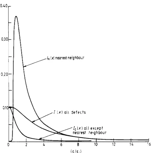
In the case described by (23) and (24) we can also calculate the distribution Io(&) from defects other than the nearest. The cosine transforms of (23) and (24) yield:

i ( x )

=

it

exp( - n x )

IN(x) = - 2 f i ker1(22/;;;) (27)

(26)

with ker'(y) as defined in Abramowitz and Stegun (1965),

8

9.9. The reverse transform must be carried out numerically, and gives the results shown in figure 1.

o.zoH

\

010

11x1 a11 d e f e c t s

c

d I I

0 2 4 6 8 10 12 16 16

i E / E l )

Figure 1. The three distributions shown are for a l / r 3 interaction with defects of both signs. I(&) is the full distribution, Iv(E) that from the nearest defect, and IO(&) from all defects but the nearest. The numerical inversion for l i s difficult technically. so that. whilst the resulting curve is basically correct, it may be inaccurate in detail.

Case 111. Assume (13) is replaced by some other monotonic power law E = q ( r ) , so that q - l ( & ) gives a single value r . Define V ( E ) = dq-'(&)/d&. Then we have as the analogue of (16):

Thus, if we were to assume

E ( T ) = A exp( - p r )

and to define er = E(L) again, we should find:

z ~ ( E ) = ( 3 / p ~ ) [In(

&&)I3

exp

-

[ ~ ~ ( E J E ) ] ~

4. Discussion

4.1. Possible applications

The discussion so far has aimed mainly at clarifying contributions to random internal strain fields. In fact, such a division into components is useful in several applications. These include hopping conduction in randomly doped crystals, and certain ordering transitions for random dipolar impurities.

Calculation of hopping conduction in randomly doped insulators and semiconductors involves two configuration-dependent factors. One concerns the overlap of states associ- ated with those nearby pairs of the dopants between which hops occur. This leads to a transition matrix element MI, falling off roughly exponentially with separation R,. The other factor involves the energy difference AEll between the initial and final states. This term varies exponentially with inverse temperature. The usual analyses (Mott and Davis 1971, § 2.9) then give the limiting cases of variable-range hopping, of Miller and Abra- hams (1960) and so on.

Even for a given spacing R,, both M , and AE,l are distributed quantities. For amorphous systems, the structural disorder is important. In such cases an empirical distribution, constant near E F , is usually assumed. For randomly doped crystalline systems, the dopant-dopant interactions may be the major factor in the spread of MI,

and AE,,

.

If so, the distributions of M , and of A E , can be obtained using the arguments

of

0

2.4. In principle, one can predict both the absolute value of the density of states and the qualitative shape of the distribution; this may permit a quantitative prediction of the hopping conductivity which improves on some current models.

iside function. In principle, these might be solved to deduce a concentration below which no phase transition is expected. In practice some generalisation is needed, since site exclusion becomes important at about the concentrations of interest.

4 . 2 . Related distributions

The distributions we have calculated are those of a scalar E . Frequently, the variable of interest is a vector (like an electric field) or a tensor (e.g. a strain). There are then two types of distribution: one is the projection of the vector onto a specific direction, i.e.

q,

=

Xz

a,u,, with /a,/2 = 1, the other the magnitude of the vector irrespective of direc- tion, i.e. ~m

=

(I:

l~,l’)’’~.

Here a is a unit vector; there are obvious generalisations for tensor quantities. Chandrasekhar (1943, § IV.2) shows that the two distributions are related by:

I,( E ) = 4Jd$lp( E ) ₍₃₁₎

in three dimensions. This has one obvious consequence: unless the distribution of the projection

q,

is singular (Ip(&)

-

E-’ at least) then

Z m ( ~ )

tends to zero with ~ m : there are essentially no sites at which the magnitude Emof the vector is zero. There are, of course, the actual defect sites themselves, though usually these are excluded from the counting because the expressions for E(z) are singular when extrapolated to defect sites.

4 . 2 . A r e there minima in &other than at defects?

In muon spin rotation one needs to know whether there are sites remote from defects where the muon will find an energy minimum. Suppose the energy of interaction with a defect is U ( r ) . Then we may seek minima in 2

U i

by looking at the distribution of forces

2 V U i = F . The minima correspond to zeros in IF1. We can see immediately from (31) and from the examples of

0

3 (and those given by Chandrasekhar (1943) or by Stoneham (1969)) that absolute minima i n U (zeros in IFI) are statistically negligible in c o m m o n random systems. This excludes ( a ) minima at defects, ( b ) the statistically negligible special cases where IF1 vanishes for fortuitous reasons, and ( c ) special potentials U ( r )

which are constant over finite volumes. We can also see from our earlier calculations here that it is the nearest defect which dominates in the force field. One may assume that the muon will move (normally by diffusion) rapidly to a nearby defect; indeed, our calculations suggest it will be the nearest defect with high probability. Trapping in isolation, other than self-trapping, is unlikely unless the strain field of an individual defect (e.g. the nearest) has large volumes of constant strain; surfaces of constant strain do not suffice.

Acknowledgments

I am most grateful to Dr J Rae for the transform giving equation (27) and to Dr J A G Temple for figure 1 and the numerical analysis on which it is based.

References

Chandrasekhar S 1943 Reo. Mod. Phys. 15 1

Garland C W, Kwiezien J Z and Damien J C 1982 Phys. Reu. B 25 5818 Hertz P 1909 Math. A n n . 67 387

Miller A and Abrahams E 1960 Phys. Rev. 120 745

Mott N F and Davis E A 1971 Electronic Processes in Non-Crystalline Materials (Oxford: Oxford University Nishiyama Z 1978 Martensitic Transformation (New York: Academic Press)

Potter R C and Anderson A C 1981 Phys. Reo. B 24 677 Stoneham A M 1969 Rev. Mod. Phys. 41 82

Stoneham A M and Bullough R 1970J. Phys. C: Solid State Phys. 3 L195 Yaouanc A 1982 Phys. Lett. 87A 423