Western University Western University
Scholarship@Western
Scholarship@Western
Electronic Thesis and Dissertation Repository
8-18-2017 10:30 AM
Turn Detection and Analysis of Turn Parameters for Driver
Turn Detection and Analysis of Turn Parameters for Driver
Characterization
Characterization
Jennifer Emily Knull
The University of Western Ontario
Supervisor Michael Bauer
The University of Western Ontario Graduate Program in Computer Science
A thesis submitted in partial fulfillment of the requirements for the degree in Master of Science © Jennifer Emily Knull 2017
Follow this and additional works at: https://ir.lib.uwo.ca/etd
Recommended Citation Recommended Citation
Knull, Jennifer Emily, "Turn Detection and Analysis of Turn Parameters for Driver Characterization" (2017). Electronic Thesis and Dissertation Repository. 4818.
https://ir.lib.uwo.ca/etd/4818
This Dissertation/Thesis is brought to you for free and open access by Scholarship@Western. It has been accepted for inclusion in Electronic Thesis and Dissertation Repository by an authorized administrator of
Abstract
Advanced Driver Assistance Systems, or ADAS, which can notify the driver of potential dangers or even perform emergency maneuvers in dangerous situations, have been shown to play a crucial role in accident prevention and driver feedback. An Intelligent ADAS, or i-ADAS, relies on information about the state of the driver, their behavior or condition, the vehicle and the environment. Understanding the behavior requires the development ofdriver models, which can help predict how a person may react in certain situations or help determine if the individual is not performing at their usual level of ability. A key element in building such models is the ability to detect and analyze common driving maneuvers, such as making turns, on an individual-by-individual basis. Thus algorithms are needed which can detect and characterize individual driving maneuvers. In this research, we present a position-based turn detection algorithm for detecting turns from vehicle data and GPS coordinates. Based on a dataset of sixteen drivers involving 278 turns, the algorithm achieves an accuracy of 97.84%. The turn parameters detected by the algorithm are then averaged for each driver and clustered using K-Means. Turn parameterst - 5 seconds are also clustered prior to each detected turn andt+5 seconds are clustered after each turn. The cluster centroids at each point in time de-termine particular driving behaviours which are summarized in four categories, and the cluster assignments are examined over time to categorize drivers into these behaviour categories. This analysis reveals two optimal times for analyzing driver behaviour. Our overall aim is to be able to build automated methods that can use this research to eventually determine characteristics of individual drivers during turns in order to build models of drivers for use with i-ADAS.
Keywords: Time series analysis, turn detection, data mining, driver characterization
Contents
Abstract i
List of Figures iv
List of Tables vi
List of Algorithms viii
List of Appendices ix
1 Introduction 1
2 Related Work 3
3 RoadLab Data 7
3.1 RoadLab . . . 7
3.2 Structure of the Data . . . 9
3.3 Relevant Data . . . 11
3.4 Data Constraints . . . 11
3.5 Related Work in RoadLab . . . 12
4 Position-Based Turn Detection 14 4.1 Concept . . . 14
4.2 Implementation . . . 18
4.2.1 main() . . . 19
4.2.2 detectT urns() anddetectT urnsRotated() . . . 19
4.2.3 mergeT urns() . . . 23
4.2.4 removeDuplicates() . . . 23
4.3 Results and Discussion . . . 25
5 Cluster Analysis 38 5.1 Preprocessing . . . 39
5.2 K-Means Clustering . . . 42
5.3 Results and Cluster Descriptions . . . 47
5.4 Driver Characterization . . . 54
5.5 Optimal Time for Analysis . . . 57
5.6 Key Observations . . . 59
6 Conclusion and Future Work 60
Bibliography 63
A Preprocessed Files for Analysis 66
B Cluster Assignments of Drivers 77
Curriculum Vitae 89
List of Figures
3.1 The RoadLab in-vehicle laboratory: a) (left): on-board computer and LCD screen, b) (center): dual stereo front visual sensors, c) (right): side stereo
visual sensors [4]. . . 7
3.2 A map view of the closed route . . . 9
4.1 Projection of the Earth overlaid with geographic latitude and longitude . . . 14
4.2 Example of vectors~uand~vwherem1andm2 are in adjacent quadrants . . . 15
4.3 Example of vectors~uand~vwherem1andm2 are in the same quadrant . . . 16
4.4 Example of an undetected turn . . . 17
4.5 Block diagram of the position-based turn detection program . . . 19
4.6 Turns that occur in a parking lot . . . 25
4.7 Plotted route of driver 1 . . . 26
4.8 Plotted route of driver 2 . . . 26
4.9 Plotted route of driver 3 with 2 FP . . . 27
4.10 Map view of driver 3 where the first false turn was detected . . . 28
4.11 Map view of driver 3 where the second false turn was detected . . . 28
4.12 Plotted route of driver 4 . . . 28
4.13 Plotted route of driver 5 . . . 29
4.14 Plotted route of driver 6 . . . 29
4.15 Plotted route of driver 7 . . . 30
4.16 Plotted route of driver 8 . . . 30
4.17 Plotted route of driver 9 . . . 31
4.18 Plotted route of driver 10 with 1 FN . . . 31
4.19 Plotted route of driver 11 . . . 32
4.20 Plotted route of driver 12 . . . 32
4.21 Plotted route of driver 13 with 1 FP and 2 FN . . . 33
4.22 Map view of driver 13 where a false turn was detected . . . 33
4.23 Plotted route of driver 14 . . . 34
4.24 Plotted route of driver 15 . . . 35
4.25 Plotted route of driver 16 . . . 35
5.1 Result of the elbow method for all drivers 5 seconds prior to all turns . . . 43
5.2 Result of the elbow method for all drivers 4 seconds prior to all turns . . . 43
5.3 Result of the elbow method for all drivers 3 seconds prior to all turns . . . 44
5.4 Result of the elbow method for all drivers 2 seconds prior to all turns . . . 44
5.5 Result of the elbow method for all drivers 1 second prior to all turns . . . 44
5.6 Result of the elbow method for all drivers during turns . . . 44
5.7 Result of the elbow method for all drivers 1 second after all turns . . . 45
5.8 Result of the elbow method for all drivers 2 seconds after all turns . . . 45
5.9 Result of the elbow method for all drivers 3 seconds after all turns . . . 45
5.10 Result of the elbow method for all drivers 4 seconds after all turns . . . 45
5.11 Result of the elbow method for all drivers 5 seconds after all turns . . . 45
List of Tables
3.1 Summary of participant information and driving conditions . . . 8
3.2 The closed route used for the RoadLab data collection . . . 9
3.3 Example of raw data frame information . . . 9
3.4 Data extracted for this research . . . 11
3.5 Example of noisy geographical data and missing data . . . 12
4.1 Results from Figures 4.2, 4.3 and 4.4 form1∗m2 . . . 17
4.2 Results from Figures 4.2, 4.3 and 4.4 when the coordinates are rotated by 45 degrees . . . 18
4.3 Raw data of driver 3 where the first false turn was detected . . . 27
4.4 Raw data of driver 3 where the second false turn was detected . . . 28
4.5 Raw data of driver 10 where a turn should have been detected . . . 31
4.6 Raw data of driver 13 where a false turn was detected . . . 32
4.7 Raw data of driver 13 where the first FN should have been detected . . . 33
4.8 Raw data of driver 13 where the second FN should have been detected . . . 34
4.9 Results of the Position-Based Turn Detection algorithm . . . 35
4.10 Results of the Position-Based Turn Detection algorithm with missed turns (due to missing data) included as actual turns . . . 36
5.1 Zero values of steering wheel position and acceleration during turns . . . 39
5.2 Summary of how the final set of descriptors are to be interpreted . . . 40
5.3 Translation of 1-second intervals to number of frames . . . 41
5.4 Silhouette scores of all analysis files for 1 to 6 clusters . . . 46
5.5 The chosenK-value(s) for each file . . . 46
5.6 Cluster centroids for cluster0 (v), cluster1 (w) and cluster2 (z) at 5 seconds pre-turns . . . 47
5.7 Angle between the 3 clusters 5 seconds pre-turns . . . 48
5.8 Cluster centroids for cluster0 (v) and cluster1 (w) . . . 48
5.9 Angle between the 2 clusters at each point in time . . . 49
5.10 Cluster assignments of drivers pre-turns of 5 seconds with 3 clusters and 5 seconds with 2 clusters . . . 50
5.11 Cluster assignments of drivers pre-turns of 4 and 3 seconds with 2 clusters . . . 50
5.12 Cluster assignments of drivers pre-turns of 2 and 1 seconds with 2 clusters . . . 51
5.13 Cluster assignments of drivers during turns and post-turns of 1 second with 2 clusters . . . 51
5.14 Cluster assignments of drivers post-turns of 2 and 3 seconds with 2 clusters . . 52
5.15 Cluster assignments of drivers post-turns of 4 and 5 seconds with 2 clusters . . 52
5.16 Observations about cluster0 and cluster1 at each point in time . . . 53
5.17 Cluster assignments over time . . . 55
5.18 The 4 categories of driving behaviour . . . 55
5.19 Driver classification . . . 57
5.20 Number of times each driver occurs in cluster0 and cluster1 . . . 58
5.21 Cluster assignment based on count . . . 58
5.22 Cluster assignments at 4 and 3 seconds pre-turns and 1 second post-turns com-pared to their categorization . . . 59
A.1 Average driver descriptors 5 seconds pre-turns . . . 66
A.2 Average driver descriptors 4 seconds pre-turns . . . 67
A.3 Average driver descriptors 3 seconds pre-turns . . . 68
A.4 Average driver descriptors 2 seconds pre-turns . . . 69
A.5 Average driver descriptors 1 second pre-turns . . . 70
A.6 Average driver descriptors during turns . . . 71
A.7 Average driver descriptors 1 second post-turns . . . 72
A.8 Average driver descriptors 2 seconds post-turns . . . 73
A.9 Average driver descriptors 3 seconds post-turns . . . 74
A.10 Average driver descriptors 4 seconds post-turns . . . 75
A.11 Average driver descriptors 5 seconds post-turns . . . 76
B.1 Cluster assignments of drivers pre-turns of 5 seconds with 3 clusters . . . 77
B.2 Cluster assignments of drivers pre-turns of 5 seconds with 2 clusters . . . 78
B.3 Cluster assignments of drivers pre-turns of 4 seconds with 2 clusters . . . 79
B.4 Cluster assignments of drivers pre-turns of 3 seconds with 2 clusters . . . 80
B.5 Cluster assignments of drivers pre-turns of 2 seconds with 2 clusters . . . 81
B.6 Cluster assignments of drivers pre-turns of 1 second with 2 clusters . . . 82
B.7 Cluster assignments of drivers during turns with 2 clusters . . . 83
B.8 Cluster assignments of drivers post-turns of 1 second with 2 clusters . . . 84
B.9 Cluster assignments of drivers post-turns of 2 seconds with 2 clusters . . . 85
B.10 Cluster assignments of drivers post-turns of 3 seconds with 2 clusters . . . 86
B.11 Cluster assignments of drivers post-turns of 4 seconds with 2 clusters . . . 87
B.12 Cluster assignments of drivers post-turns of 5 seconds with 2 clusters . . . 88
List of Algorithms
1 main(dData) . . . 19
2 detectT urns(f S eq) . . . 21
3 detectT urnsRotated(f S eq) . . . 22
4 mergeT urns(S1,S2) . . . 23
5 removeDuplicates(S) . . . 24
6 pre(t) . . . 41
7 post(t) . . . 42
List of Appendices
Appendix A Preprocessed Files for Analysis . . . 66 Appendix B Cluster Assignments of Drivers . . . 77
Chapter 1
Introduction
Driving is a risky activity that continues to be part of the everyday lives of people, whether they are a driver, passenger or pedestrian. According to the National Highway Traffic and Safety Administration (NHTSA), there were 6,296,000 police-reported motor vehicle accidents in the United States alone in 2015, with an estimated 96 fatalities per day. The cause of almost all these accidents is persistently due to driver error.
Efforts have been made by automobile manufacturers and researchers to enhance the driving experience to improve safety while driving. There are two technologies at the forefront of this revolution - autonomous vehicles and augmented vehicles. Autonomous vehicles take full control of the vehicle at all times and is, essentially, a self-driving vehicle. Here, the driver takes the role of a passenger as the vehicle drives itself. Augmented vehicles, or Advanced Driver Assistance Systems (ADAS), aid the driver as they operate the vehicle themselves, and take full control of the vehicle and decision-making when there is impending risk. ADAS can help reduce the burden of driving on humans and can improve safety by notifying the driver of potential dangers and may even perform emergency maneuvers in dangerous situations. ADASs have been shown to play a crucial role in accident prevention and driver feedback.
Intelligent ADAS, or i-ADAS, relies on information about the state of the driver, his or her behaviour or condition, the vehicle and the environment. Understanding the state of a driver or their behaviour requires the development ofdriver models, which can predict driver behaviour in certain situations based on their performance. These driver models must be built dynami-cally and adhere to specific individual behaviours and characteristics, as each driver can react differently given similar situations.
A key element in building such models is the ability to detect and analyze common driving maneuvers, such as making turns from one road to another, on an individual-by-individual basis. Analyzing these driving maneuvers then become the building blocks to creating dynamic driver models to characterize drivers. The challenge to analyzing driver behaviour is to consider the driving environment at all times; any triggers or outside influences that can explain the behaviour. Driver behaviour can greatly vary leading up to a turn and coming out of a turn, but it is believed that the environment and driving conditions are more consistently similar during a turn. This is why turns will be the driving maneuver analyzed for this research to help
2 Chapter1. Introduction
understand driving behaviour, with a strict focus on vehicle data that is not computationally expensive.
For any driving maneuver, algorithms are needed to detect and characterize these maneuvers on individual drivers. In this paper, a position-based turn detection (PBTD) algorithm will be employed to detect turns from vehicle data. This algorithm is used for post processing of turn data before, during, and after a turn maneuver. The overall aim is provide the capability of building automated methods that will use the PBTD algorithm to determine characteristics of individual drivers throughout turns. These methods are intended to help build models of drivers.
Chapter 2
Related Work
Driver modeling, as the name suggests, tries to model driver behaviour in various driving sit-uations. Driver modeling is very broad and there has been a variety of research over the past many years. Central to the discussion of driving models is the notion of a driving maneuver. A specific move or series of moves in driving is termed amaneuver. Driving maneuvers can be defined based on traffic and road infrastructure. Driving maneuvers can include “following”, “turning at intersection”, “changing lanes”, “reacting to an obstacle”, etc. These maneuvers can be differentiated by situational factors, such as the type of road, speed limit, number of lanes and the existence of other vehicles, pedestrians, traffic signs or traffic lights ahead of the vehicle.
Plochl and Edelmann [23] provide an overview of different driving models. They divide the models into four categories:
• Focus on the vehicle. The vehicle is the main goal of the model. In this case, the driver model usually serves as part of the closed loop testing of vehicle performance under various driving conditions.
• Focus on the driver. In this case the driver is the target. This includes efforts to model aspects such as driving style or psychological states while driving, such as stress or distraction.
• Focus on the vehicle/driver combination. This is really a combination of the two previous areas where the focus is on the interaction between the driver and the vehicle.
• Focus on the environment/traffic. These models simulate traffic conditions and focus on broader traffic/driving issues.
In this work, we concentrate on those works that focus on the driver or on a driver and vehicle combination.
Following Plochl and Edelmann [23], the research in this area falls into two broad subareas: a) understanding the driver and (the individual) driver behaviour (our particular focus) and b) path and speed planning, and optimized driver/driving behaviour. The first is related to modeling
4 Chapter2. RelatedWork
how a person drives a vehicle, i.e. how they execute maneuvers - this is the focus of our work and we shall restrict our review of related work to this area.
In turn, driver behaviour models can be grouped into two categories [2]: cognitive driver mod-els and behaviourist driver modmod-els. Cognitive driver modmod-els are based on human psychological behaviours and pay attention to, for example, mental and attentional features that a driver shows in performing different maneuvers. Behaviourist models utilize the information about the environment surrounding the driver, including vehicles, pedestrians and other objects in the road. Most of the proposed methods in this area are based on one of these two categories, but ultimately a combination of information in both categories can be more helpful and practical in understanding driver behaviour and predicting the most probable next maneuver.
We first consider work that falls into the behaviourist class (though in many cases this sepa-ration is not exact). Behaviourist driver models try to model how the driver interacts with the surrounding environment including the other vehicles and also his vehicle parts, such as brake and accelerator pedals, turn signals, steering wheel and other senors/actuators within vehicles. Modern vehicles, for example, are already equipped with some cameras and sensors to measure the internal vehicular information. Radar systems for detecting distance, lidar systems [18] for obstacle detection, visual systems [31] for detecting road objects [1] and vehicle navigation systems, such as GPS [17], have been used in advanced driving assistance systems.
Driver behaviour can be predicted by knowing how a driver acts in certain driving tasks, such as turning, lane changing and overtaking a vehicle. Chandler, et al. [7] implemented a vehicle-following model and used data from experiments with real vehicles to set the model’s param-eters. Ioannou [21] implemented an Automatic Cruise Control (ACC) system and compared it to three different human driver models. The results were that the ACC system was able to provide safer driving. A hybrid, three-layered ACC system based on fuzzy logic and neural networks has also been implemented by Dermann et al. [9].
Other maneuvers have been also studied: emergency braking [30, 29], lane change [14, 20], and turning at intersections [6, 8]. Predicting the driver’s intention could provide valuable information in the context of ADAS.
A number of methods have also been implemented for assessing the driver’s sleepiness. Most of them utilize some features in the driver’s face through video cameras and use eye and eyelid movements [5, 11, 22, 28] or head movements [5, 11, 12] or some combination of both to infer sleepiness. A few indirect algorithms, usually using steering behaviour in the context of lane keeping [28, 27] have also been developed.
5
(stress, fatigue, alcohol, etc.) and so on [10]. Metari et al. [21] analyzed the cephalo-ocular behaviour of drivers in vehicle/road events, such as overtaking and crossing an intersection. This work was specifically concerned with finding the relationship between vision behaviour of older drivers and their actions in road events. They posited that the cephalo-ocular informa-tion can be related to the driving maneuvers a driver decides to make. Some other researchers have also tested the impact of eye movements on control of actions in everyday events, such as driving [15, 16].
Analysis of driver behaviour within the context of a cognitive architecture can be important in determining the motivation behind making a specific decision in a driving event [25]. For example, when a driver decides to make a left or right turn, visual information can show that they look at the mirrors, blind spot, traffic and so on. Baumann et al. [3] model the situation awareness of a driver in a cognitive architecture with the aim of assisting an i-ADAS to assist the driver during driving and to augment safety. Despite the fact that visual information, such as gaze tracking, is important in predicting driver behaviour, little research has been done in this domain. The main reason that these models have not received much attention are the challenges in measuring cognitive behaviour in such complex systems.
It is clear that details of driving maneuvers have been considered essential in the development of driver models. Much of this work, however, has relied on the researcher to first identify such maneuvers, often manually, which are then used in subsequent analyses. To be able to infer models of individual drivers, driving maneuvers must first be determined in situ and then used to build the model. A first step is to be able to identify such maneuvers from the data available from the vehicle, which is covered in this thesis.
Another area that has received attention by researchers is the detection of driving maneuvers. Kasper et al. [13] provide a novel approach for detecting lane-change maneuvers in structured highway scenarios using object-oriented Bayesian Networks (OOBNs) with a vehicle-lane re-lation. Mandalia et al. [19] proposes a technique for observing driver intent to change lanes using a support vector machine (SVM). Alternatively, Weiss et al. [32] detect lane changes of an observed target vehicle with a motion model that detects significant variability in lateral direction. A second motion model also determines if the target vehicle is staying within the lane by looking for high variability in longitudinal direction. Salvucci et al. [26] introduces a robust, real-time system for detecting lane changes. In this work, a model-tracing system simulates driver intention and consequent behaviour based on a simplified, previously vali-dated computational model of driver behaviour. The system compares the model’s simulated behavour with actual observed driver behaviour, and constantly infer the driver’s unobservable intentions from their observable actions.
6 Chapter2. RelatedWork
Chapter 3
RoadLab Data
3.1
RoadLab
RoadLab is an initiative that provides data for the development of i-ADAS. The aim is to support research for i-ADAS cognizant of driver behaviour, intent, surrounding traffic and general driving conditions to help alleviate injuries caused by vehicle accidents. The initial dataset provides a resource for researchers to analyze driver data with the hope of reducing the social and economic costs caused by human errors made while driving.
RoadLab data is collected by an in-vehicle laboratory instrumented with an on-board diagnos-tic system (OBD-II) using the CANbus protocol as described in [4] (see Figure 3.1). The instrumentation was able to retrieve video sequences of the driving environment in front of the vehicle, ocular behaviour of the driver such as driver gaze, geographic position of the vehicle using GPS units, and data describing the state of all the vehicle parameters such as brake pedal position, steering wheel position, etc. This research has its primary focus on the vehicular data for turn detection.
Figure 3.1: The RoadLab in-vehicle laboratory:a) (left):on-board computer and LCD screen,
b) (center): dual stereo front visual sensors,c) (right): side stereo visual sensors [4].
The data comes from a study that was conducted on 16 individuals between the ages of 20 and 47 from London, Ontario; a summary of the participants and driving conditions is provided in
8 Chapter3. RoadLabData
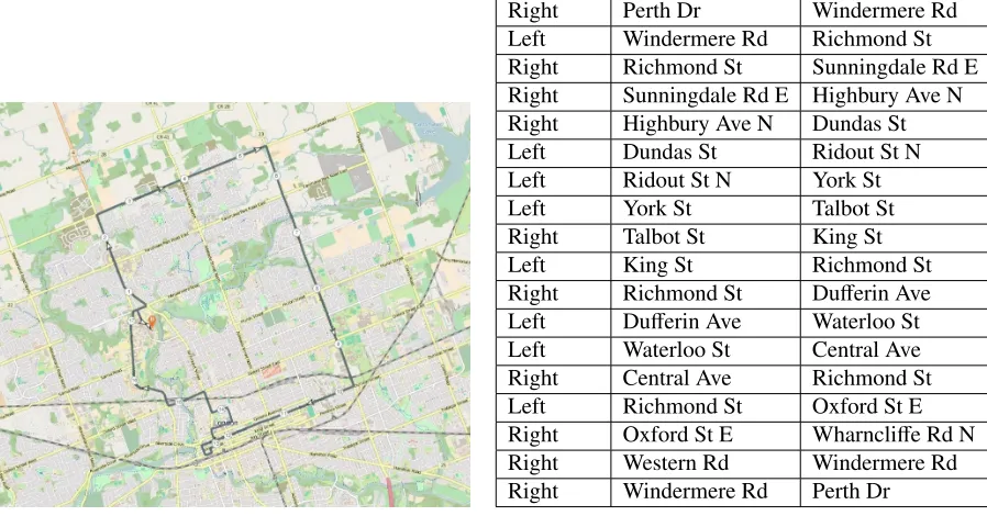
Table 3.1. Each participant used the RoadLab vehicle to drive along a predetermined route, shown in Figure 3.2 and Table 3.2, and were accompanied by two observants. One observant was present to monitor the equipment and ensure its proper performance. The second observant helped navigate the participants along the chosen route.
Participant Date Time Weather Conditions Age Gender
1 2012-08-24 13:15 29C, Sunny 37 M
2 2012-08-24 15:30 31C, Sunny 37 M
3 2012-08-30 12:15 23C, Sunny 41 F
4 2012-08-31 11:00 24C, Sunny 41 M
5 2012-09-05 12:05 27C, Partially Cloudy 37 F 6 2012-09-10 13:00 21C, Partially Cloudy 22 F
7 2012-09-12 11:30 21C, Sunny 31 F
8 2012-09-12 14:45 27C, Sunny 21 M
9 2012-09-17 13:00 24C, Partially Cloudy 21 F
10 2012-09-19 09:30 8C, Sunny 20 M
11 2012-09-19 14:45 12C, Sunny 22 F
12 2012-09-21 11:45 18C, Partially Sunny 24 F 13 2012-09-21 14:45 19C, Partially Sunny 23 M
14 2012-09-24 11:00 7C, Sunny 47 F
3.2. Structure of theData 9
Figure 3.2: A map view of the closed route
Turn Type Start Road End Road
Right Perth Dr Windermere Rd
Left Windermere Rd Richmond St Right Richmond St Sunningdale Rd E Right Sunningdale Rd E Highbury Ave N Right Highbury Ave N Dundas St
Left Dundas St Ridout St N
Left Ridout St N York St
Left York St Talbot St
Right Talbot St King St
Left King St Richmond St
Right Richmond St Dufferin Ave Left Dufferin Ave Waterloo St
Left Waterloo St Central Ave
Right Central Ave Richmond St
Left Richmond St Oxford St E
Right Oxford St E Wharncliffe Rd N
Right Western Rd Windermere Rd
Right Windermere Rd Perth Dr
Table 3.2: The closed route used for the Road-Lab data collection
3.2
Structure of the Data
The data from RoadLab has been collected in real-time as each participant, or driver, navi-gated along the route. There is a total of approximately 60 minutes of driving data for each participant, which varies based on how long it took for each driver to complete the route. The time-series data was collected at a sampling rate of 15Hz, which were captured into data frames. Each data frame represents approximately 151 seconds of data, and contains current contextual information about the vehicle and its geographical position.
Frame Number Timestamp Latitude Longitude GPS Speed Speed
1 588534044 43.0103 -81.2711 0 0
2 588580132 43.0103 -81.2711 0 0
3 588617063 43.0103 -81.2711 0 0
Brake Pressure Gas Pressure Steering Wheel
Position
Left Turn Signal
Right Turn Signal
156 0 -567 0 0
155 0 -567 0 0
155 0 -567 0 0
10 Chapter3. RoadLabData
Table 3.3 contains three sample data frames found in the RoadLab data. Every data frame contains a:
• Frame Number:an index that indicates the current frame.
• Timestamp: this represents the time of occurrence of the information within the frame.
• Latitude: geographic latitude value in signed degrees format with four decimal preci-sion.
• Longitude:geographic longitude value in signed degrees format with four decimal pre-cision.
• GPS Speed: the speed of the vehicle in km/hr, measured by satellite.
• Speed:the speed of the vehicle in km/hr, measured by vehicle sensors.
• Brake Pressure:amount of pressure on the brake pedal, ranging from 0 (no pressure) to 156 (maximum pressure).
• Gas Pressure:amount of pressure on the gas pedal, ranging from 0 (no pressure) to 187 (maximum pressure).
• Steering Wheel Position:represents the angle of the steering wheel, ranging from -567 to 579. A negative angle indicates the steering wheel is left of the centre, or rest, position, and a positive angle indicates the right.
• Left Turn Signal: this value is either 0 if the left turn signal is off, or 1 if the left turn signal is on.
• Right Turn Signal: this value is either 0 if the right turn signal is off, or 1 if the right turn signal is on.
The values of brake pressure, gas pressure and steering wheel position were generated from CANbus signals and have no specific units.
3.3. RelevantData 11
3.3
Relevant Data
This research specially uses latitude, longitude and steering wheel position to detect all turns along the route taken by the RoadLab vehicle. The following parameters are used as descriptors for all the detected turns: speed, brake pressure, gas pressure and steering wheel position. These are the same parameters that were used in the previous example. These descriptors also provide a basis for deriving more data such as acceleration, duration, and average, standard deviation, skewness and kurtosis.
Frame Number Timestamp Latitude Longitude GPS Speed Speed
1 588534044 43.0103 -81.2711 0 0
2 588580132 43.0103 -81.2711 0 0
3 588617063 43.0103 -81.2711 0 0
Brake Pressure Gas Pressure Steering Wheel
Position
Left Turn Signal
Right Turn Signal
156 0 -567 0 0
155 0 -567 0 0
155 0 -567 0 0
Table 3.4: Data extracted for this research
A decision has been made to exclude GPS speed from the analysis. It has been found that this parameter is subject to noise since it is measured by satellite. It is more accurate to use sensors on the vehicle to measure speed, so this measurement of speed will be used. Left and right turn signals are also excluded. The left and right turn signals can be unreliable since they are triggered by the driver. Steering wheel position will act as a substitute for these flags, and a threshold will indicate a left turn or a right turn.
Table 3.4 highlights the set of parameters that will be used for this research. Frame number was not selected for analysis, but will be used in the algorithms for turn detection.
3.4
Data Constraints
There are several constraints that need to be considered. The RoadLab dataset excels with depth, but lacks in breadth. There is approximately 54,000 frames of data across all 16 drivers, and this provides ample information to conduct analysis. However, the sample size of the study contains only 16 drivers, which can make it difficult for the results to provide conclusions and concrete assumptions for driver characterization.
12 Chapter3. RoadLabData
Frame Number Timestamp Latitude Longitude GPS Speed Speed
23448 1606770659 43.0433 -81.2270 44 47
23449 1632795784 43.0403 -81.2255 44 44
Brake Pressure Gas Pressure Steering Wheel
Position
Left Turn Signal
Right Turn Signal
1 57 0 0 0
1 35 -12 0 0
Table 3.5: Example of noisy geographical data and missing data
Geographical data is retrieved by satellite using the GPS. GPS is vulnerable to signal inter-ference for different reasons, which causes sporadic jumps in latitude and longitude readings. The turn detection software eliminates risk of this affecting the results by enforcing a thresh-old. Missing data can also occur when the in-vehicle laboratory goes offline due to a technical issue. Any turns executed during this state cannot be detected and will be missing from the analysis. Table 3.5 provides an example from the raw data. There should be an incremental increase or decrease (or no difference at all) between latitude and longitude values going from one frame to the next. In this example, there is a 0.003 difference in latitude values and a 0.0015 difference in longitude values. This much of a difference entirely displaces the vehicle approximately 350 metres in 1/15th of a second, which is most likely not the case. Because the turn detection algorithm uses a position-based approach, this difference is considered to be noisy. From an analysis perspective, there is a gap between these two data frames, so there is also missing data.
Lastly, the study was conducted under supervision, which may have caused the participants to behave differently and drive less naturally, in contrast to being unsupervised. This issue cannot be avoided since without the instrumentation, there would be no data. The RoadLab instrumentation cannot be legally installed on an individual’s vehicle without their consent. Each participant was also guided along the route by one observant. There are instances where the participants deviated slightly away from the route due to erroneous commands. Because of this, the routes for some participants are slightly different from the predetermined route they were meant to follow. All detected turns that do not belong in the route will also be included in the analysis, as this research aims to characterize drivers, not turns.
3.5
Related Work in RoadLab
3.5. RelatedWork inRoadLab 13
Chapter 4
Position-Based Turn Detection
4.1
Concept
As a vehicle travels along the Earth, its position can be uniquely represented as a latitude and longitude coordinate using GPS. This coordinate maps to only one location, making the position of any vehicle identifiable and traceable. The idea behind the position-based approach is to use latitude, ϕ, and longitude values, λ, to identify a change from one road to another. Since GPS can pinpoint any location, it is assumed that we can analyze the coordinates that represent these locations to detect turns.
The RoadLAB dataset provides ϕ and λ in signed degrees format of up to (and including) four decimal places. This degree of precision can identify individual streets and land parcels according to the qualitative scale, which, shown later in this work, provides enough accuracy for turn indentification.
Geographic latitude and longitude can be mapped to a Cartesian coordinate system (see Figure 4.1), in whichϕ represents a numerical value along the y-axis andλrepresents a value along the x-axis. Turns will be detected, using the coordinate system, by specific fluctuations in∆ϕ and∆λ.
Figure 4.1: Projection of the Earth overlaid with geographic latitude and longitude
4.1. Concept 15
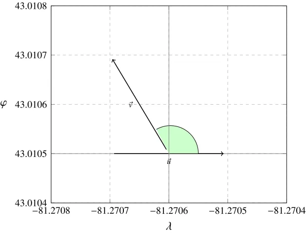
As a vehicle travels along a path, its position vector can be calculated. This vector signifies the direction of travel using two (λ, ϕ) endponts. The position-based algorithm takes two position vectors,~uand~v, when there is a change in endpoints, and if the angle between~uand~vis greater or equal to 90 degrees then there is evidence of a turn.
−81.2708 −81.2707 −81.2706 −81.2705 −81.2704 43.0104
43.0105 43.0106 43.0107 43.0108
~u ~v
λ ϕ
Figure 4.2: Example of vectors~uand~vwherem1andm2 are in adjacent quadrants
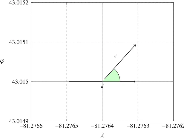
Two slopes,m1andm2, are used to describe how much of a change there is in direction between one position vector and the other. Instead of calculating the angle between~u and~v, we can determine if there is a shift between quadrants in the coordinate system (see Figures 4.2 and 4.3). Each quadrant is separated by 90 degrees, so ifm1 andm2define two adjacent quadrants, then a turn has occurred.
The values m1 and m2 are defined as the change in latitude values, ∆ϕ, over the change in longitude values,∆λ:
m1=
ϕ2−ϕ1
λ2−λ1
(4.1)
and
m2 =
ϕ3−ϕ2
λ3−λ2
. (4.2)
16 Chapter4. Position-BasedTurnDetection
1. m1andm2 are both positive. 2. m1andm2 are both negative. 3. m1is positive andm2 is negative. 4. m1is negative andm2is positive.
Cases 1 and 2 suggest that the slopes are not in adjacent quadrants. This is because there would be an opposition in sign if they were. Cases 3 and 4 suggest that the slopes are adjacent, in which cases a turn is detected.
−81.2766 −81.2765 −81.2764 −81.2763 −81.2762 43.0149
43.015 43.0151 43.0152
~u ~ v
λ ϕ
Figure 4.3: Example of vectors~uand~vwherem1andm2are in the same quadrant
Since only the signs are being considered, the formulas form1andm2 can be rewritten as:
m1 = (ϕ2−ϕ1)(λ2−λ1) (4.3)
and
m2 =(ϕ3−ϕ2)(λ3−λ2), (4.4)
which solves the division by zero problem. This narrows the classification to two cases: 1. m1∗m2is negative, and
4.1. Concept 17
Here, Case 1 identifies a turn maneuver and Case 2 indicates otherwise.
−81.2767 −81.2766 −81.2765 −81.2764 43.0147
43.0148 43.0149 43.015 43.0151
~
u ~v
λ ϕ
(a)~uand~vwherem1andm2are in the same quad-rant
(b) Western Rd. to Windermere Rd.
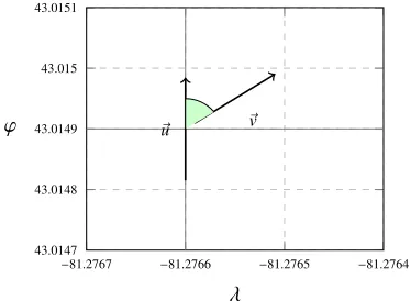
Figure 4.4: Example of an undetected turn
Figure ϕ1 ϕ2 ϕ3 λ1 λ2 λ3 m1∗m2
4.2 43.0105 43.0105 43.0107 -81.2707 -81.2706 -81.2707 negative 4.3 43.015 43.015 43.0151 -81.2765 -81.2764 -81.2763 positive 4.4 43.0148 43.0149 43.0150 -81.2766 -81.2766 -81.2765 positive
Table 4.1: Results from Figures 4.2, 4.3 and 4.4 form1∗m2
It is assumed that turn maneuvers take place at 90 degrees or more, but it’s possible for them to occur at<90 degrees and remain in the same quadrant (see Figure 4.4). A quick fix would be to rotate (λ1, ϕ1), (λ2, ϕ2) and (λ3, ϕ3) by 45 degrees using this formula:
"
cos 45 −sin 45 sin 45 cos 45
# " ∆λ ∆ϕ
#
(4.5)
yielding
∆λ0 =
18 Chapter4. Position-BasedTurnDetection
and
∆ϕ0=
0.707∆λ+0.707∆ϕ. (4.7)
Thenm1andm2can be calculated to determine a turn:
m1∗m2= ∆ϕ02∆ϕ
0
1∆λ
0
2∆λ
0
1. (4.8)
Figure ϕ1 ϕ2 ϕ3 λ1 λ2 λ3 m1∗m2
4.2 43.0105 43.0105 43.0107 -81.2707 -81.2706 -81.2707 positive 4.3 43.015 43.015 43.0151 -81.2765 -81.2764 -81.2763 positive 4.4 43.0148 43.0149 43.0150 -81.2766 -81.2766 -81.2765 negative Table 4.2: Results from Figures 4.2, 4.3 and 4.4 when the coordinates are rotated by 45 degrees
The results from Table 4.2 show that the turn from Western Rd. to Windermere Rd. is now detected. However the results from Figure 4.2 have changed. By rotating all the coordinates by 45 degrees, the classification has changed from a turn to no turn at all. This is why, described further in the next section, the set of results from the original calculation, S1, and the set of
results from rotating the coordinates,S2, will constitute all turns detected by the algorithm:
S1∪S2. (4.9)
By taking the union, a turn is detected from Figure 4.2 and Figure 4.4, and Figure 4.3 does not count as a turn. This is the correct turn identification for these three examples.
4.2
Implementation
The turn detection algorithm consists of three stages, with the amalgamation of these stages producing the final set of turns for each driver. The three stages are:
1. Turn Detection
(a) Without rotation. (b) With rotation. 2. Merge Turns 3. Remove Duplicates
4.2. Implementation 19
Detect Turns
Sequence of Frames
Merge S1
andS2
Remove Duplicates
Turn Events S1
S2
S1∪S2
Figure 4.5: Block diagram of the position-based turn detection program
4.2.1
main
()
The main program loops through the raw data for all 16 drivers and generates a file containing the detected turns with comma-separated values. The sequence of frames for each driver is supplied to the main program, which is then passed to the detection methods, detectT urns() and detectT urnsRotated(). These two methods use the sequence of frames to detect turns.
detectT urns() anddetectT urnsRotated() will produce different results, which is whymergeT urns() takes these results and combines them. There will also be turns detected by both methods, as seen at the end of the previous section, so theremoveDuplicates() method is called to ensure that each turn in the set is unique. Lastly, the final set is saved to a file.
Algorithm 1:main(dData)
1 Input: dData% this contains raw data about each driver, shown in Table 3.1 2 Output: 16 files of turn events% where each file contains turn events of the driver 3 fordriver in dDatado
4 S1 ←detectT urns(driver.f S eq())
5 S2 ←detectT urnsRotated(driver.f S eq()) 6 S ←mergeT urns(S1,S2)
7 S0 ←removeDuplicates(S)
8 S0.write()
4.2.2
detectT urns
()
and
detectT urnsRotated
()
Algorithm 2 and Algorithm 3 are implementations of the concepts discussed in the previous section. Both methods readFS eqframe by frame, and keep track of the latitude and longitude values of the current frame and the previous frame: λ1,ϕ1,λ2 andϕ2. The algorithm looks for
a change in latitude values, 4ϕ , 0, and a change in longitude values, 4λ , 0, between the previous frame and the current frame. This change indicates that the vehicle has moved to a different geographical location, and this must be checked to see if a turn could have occurred. The change in latitude and longitude is compared against aNOIS Y T RHES HOLDwhich has been set to 0.0002. This threshold is used to avoid any false positives that may cause a turn to be detected when there is missing data. The latitude and longitude values were examined and they do not increase or decrease by more than 0.0001. NOIS Y T HRES HOLDis thus set to 0.0002 to ensure that the vehicle is travelling incrementally when a change is detected.
20 Chapter4. Position-BasedTurnDetection
that a difference has occurred in Line 13 and this difference is valid, the flag is checked to determine if this could be a) the start of a turn, or b) the end of a turn. A start of a turn means thatchange = Falsesince a difference has not yet been detected, and an end of a turn means thatchange=T ruesince the program has already detected a difference in geographical location and this could mean the end of a turn.
When the start of a turn is identified, the program saves the value ofm1at Line 18, which is used
later when the program detects a second change in latitude and longitude. When a possible end of a turn is identified, this could mean either a) a turn is detected, or b) a turn is not detected and the vehicle is simply travelling along a straight path. In both cases,m2 is calculated and
the program checksm1∗m2. Ifm1∗m2 ≤0 then the program detects a turn. Before this turn is
added toS1(S2for Algorithm 3), the absolute average steering wheel position between fstartto
fend needs to be checked against a BEND T HRES HOLD. BEND T HRES HOLDis needed to differentiate actual turns from bends in the road. Without this threshold some bends may be detected as turns if given the properλ1, ϕ1, λ2 and ϕ2. An example of a detected bend is
the one north of Oxford Street along Western Road. The value ofBEND T HRES HOLDwas chosen by trial and error. The threshold is set to 40 for Algorithm 2 and 100 for Algorithm 3 as they proved most successful in identifying turns and excluding bends. Ifm1 ∗m2 ≤ 0 and the
absolute value of the average steering wheel position is less thanBEND T HRES HOLD, then the turn event is added toS1(S2for Algorithm 3). The methodwheelDirection() calculates the
average steering wheel position from fstart to fend. If the average is negative, then the steering wheel position was, on average, to the left of the center position which signifies a left turn. If the average was positive, then wheelDirection() would indicate that, on average, the steering wheel was to the right of the center and label a right turn.
Ifm1∗m2 > 0 then the program does not detect a turn. In this case, the vehicle is continuing
along a straight path. However, this could also indicate the start of a new turn. The program does not ignore the possibility of a new turn, so it setsm1tom2andchangeremains to beT rue.
Based on the turn detection program, the start of an identified turn is defined as the first change in latitude or longitude values. The end of the turn is defined as the second change in latitude or longitude values. The frame number of fstart and fend are converted to a time, in seconds, using this formula:
t1 =
fstart
15 (4.10)
and
t2 =
fend
15 , (4.11)
and their difference constitutes the duration of the turn in seconds:
4.2. Implementation 21
Algorithm 2:detectT urns(f S eq)
1 Input: fSeq% sequence of frames
2 Output: S1 % set of turns containing start and end frames, start and end latitude and
longitude
3 S1 ←φ
4 f1 ← f S eq[1] % first frame
5 ϕ1=latitude(f1) 6 λ1=longitude(f1)
7 change← False% True if possible turn detected 8 for f in f S eqdo
9 ϕ2 =latitude(f) 10 λ2=longitude(f)
11 4ϕ=ϕ2−ϕ1 12 4λ=λ2−λ1
13 if (4ϕ, 0or4λ, 0)and4ϕ <NOIS Y T HRES HOLD and
4λ < NOIS Y T HRES HOLDthen
14 % change in latitude or longitude is detected
15 if change==Falsethen
16 % possible start of a turn
17 change←T rue
18 m1 ← 4ϕ4λ
19 fstart ← f
20 ϕ1 =ϕ2
21 λ1=λ2
22 else
23 % possible end of a turn
24 fend ← f
25 m2 ← 4ϕ4λ
26 if m1∗m2≤ 0and averageWheel(fstart, fend)< BEND T HRES HOLDthen
27 % turn detected
28 turn type←wheelDirection(fstart, fend)
29 turn←(fstart, fend,turn type)
30 S1.append(turn)
31 change← False
32 else
33 % turn not detected, possible start of a turn 34 fstart ← fend
35 m1=m2
36 ϕ1=ϕ2
37 λ1=λ2
38 else
39 ϕ1 =ϕ2
22 Chapter4. Position-BasedTurnDetection
Algorithm 3:detectT urnsRotated(f S eq)
1 Input: fSeq% sequence of frames
2 Output: S2 % set of turns containing start and end frames, start and end latitude and
longitude
3 S2 ←φ
4 f1 ← f S eq[1] % first frame
5 ϕ1=latitude(f1) 6 λ1=longitude(f1)
7 change← False% True if possible turn detected 8 for f in f S eqdo
9 ϕ2 =latitude(f) 10 λ2=longitude(f)
11 4ϕ=ϕ2−ϕ1 12 4λ=λ2−λ1
13 if (4ϕ, 0or4λ, 0)and4ϕ <NOIS Y T HRES HOLD and
4λ < NOIS Y T HRES HOLDthen
14 % change in latitude or longitude is detected
15 if change==Falsethen
16 % possible start of a turn
17 change←T rue
18 4λ0 ←0.7074λ−0.7074ϕ 19 4ϕ0 ←0.7074λ+0.7074ϕ
20 m1 ← 4ϕ04λ0
21 fstart ← f
22 ϕ1 =ϕ2
23 λ1=λ2
24 else
25 % possible end of a turn
26 fend ← f
27 4λ0 ←0.7074λ−0.7074ϕ 28 4ϕ0 ←0.7074λ+0.7074ϕ
29 m2 ← 4ϕ04λ0
30 if m1∗m2≤ 0and averageWheel(fstart, fend)< BEND T HRES HOLDthen
31 % turn detected
32 turn type←wheelDirection(fstart, fend)
33 turn←(fstart, fend,turn type)
34 S2.append(turn)
35 change← False
36 else
37 % turn not detected, possible start of a turn 38 fstart ← fend
39 m1=m2
40 ϕ1=ϕ2
41 λ1=λ2
42 else
43 ϕ1 =ϕ2
4.2. Implementation 23
Algorithm 2 detects turns directly from the sequence of frames for each driver. Algorithm 3 does the same, except the coordinates are rotated by 45 degrees. This is so wide turns, such as the turn from Western Road to Windermere Road, can be detected even though the angle between~uand~v is less than 90 degrees and remain in the same quadrant. Lines 18 and 19, and 27 and 28 in Algorithm 3 rotate the latitude and longitude coordinates before calculating
m1∗m2.
4.2.3
mergeT urns
()
The previous section observed that the results of Algorithm 2 and Algorithm 3 are different, and, thus, need to be combined using a merging algorithm.
The merging algorithm reads all turn events fromS1 and S2 and stores them in a dictionary,
ordered by the starting frame of the turn (see Lines 6 and 8). They are stored by starting frame so that the dictionary can be sorted at Line 9. The starting frame of a turn indicates the time at which the turn started (see Equation 4.10). The method produces a list of turns, ordered by occurrence, that were detected by both Algorithm 2 and Algorithm 3.
Algorithm 4:mergeT urns(S1,S2)
1 Input: S1 and S2% two sets of turn events 2 Output: S % the combined set of turn events
3 S ←φ
4 turnDict ←φ% dictionary of turns stored by start frame 5 forturn in S1 do
6 turnDict[turn.startFrame()]←turn 7 forturn in S2 do
8 turnDict[turn.startFrame()]←turn 9 S ← sort(turnDict)
4.2.4
removeDuplicates
()
Algorithm 2 and Algorithm 3 produce different sets of turns, however, there are also similarities between S1 and S2, i.e. they can both detect turns that represent the same turn event. This
results in a set of duplicate turns when the merge method unifies the sets.
TheremoveDuplicates() method extracts distinct turn events from the combined set of turns. This will represent the final the set of turns to write to the file. It reads the first two turns from
S and tests whether the two turns are the same turn or two separate turns. The start frame and end frame of both turns are evaluated to determine the closeness between the turns. A
24 Chapter4. Position-BasedTurnDetection
FRAME T HRES HOLDwas tested on values between a 15 and 225 frame difference, which
is equivalent to 1 to 15 seconds. It was assumed that turns could not occur back-to-back in less than 1 second. The testing proved that 170 was the most optimal value forFRAME T HRES HOLD. It was found that if it was more than 170 the method would start merging turns that were
actu-ally different. This proved that turns were separated by at least 11.3 seconds. IfFRAME T HRES HOLD
was set to a value less than 170, the method would separate turns that were the same, thus leav-ing duplicate turns in the final set.
If the first two turn events represent different turns, then both turn events were added toS0. If they are duplicates of the same turn, then the second turn was added toS0(see Line 10). There
is no advantage to taking one turn over the other, soturn2 was chosen by default. The method proceeds to read the rest of the turn events from S, one turn at a time. It updates turn1 and
turn2 by settingturn1 toturn2 andturn2 to the new turn being read. Since the turns inS are sorted by occurrence, it is suitable to read and compare turns in sequential pairs. If there are duplicate turns, then they will be listed one after the other inS.
Ifturn1 andturn2 are separate turn events, then onlyturn2 will be added toS0. If they are the
same event, none of them are added toS0. In the loop, the second turn is the only one copied toS0, so if the turns are the same, they are essentially skipped so that there is no duplicate of
turn2 inS0. Remember,
turn2 is reset toturn1 at the start of the loop.
Algorithm 5:removeDuplicates(S)
1 Input: S % set of turn events
2 Output: S0 % set of distinct turn events 3 S0 ←φ
4 turn1←S.readT urn() 5 turn2←S.readT urn()
6 if !(abs(turn1.startFrame()−turn2.startFrame())< FRAME T RHES HOLD or abs(turn1.endFrame()−turn2.endFrame())< FRAME T HRES HOLD)then 7 S0.append(turn1)
8 S0.append(turn2) 9 else
10 S0.append(turn2) 11 forturn in S do
12 turn1←turn2
13 turn2←turn
14 if !(abs(turn1.startFrame()−turn2.startFrame())< FRAME T RHES HOLD or abs(turn1.endFrame()−turn2.endFrame())< FRAME T HRES HOLD)then
4.3. Results andDiscussion 25
4.3
Results and Discussion
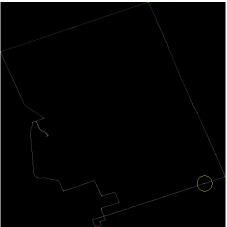
After executingmain(), which executes detectT urns(), detectT urnsRotated(), mergeT urns() and removeDuplicates(), 16 files of turn events were generated where each file contains the turn events of its respective driver. Figures 4.7 to 4.25 show the plotted route based on the GPS data. Overlying these routes are red and green points. A red point represents a left turn that was detected by the PBTD method and a green point represents a right turn. These turns were taken from the driver’s turn events file provided bymain().
Any turns that were detected going in and out of parking lots were excluded, along with turns occurring in a parking lot. This was to prevent these turns from skewing the results of the analysis. The points circled in Figure 4.6 were excluded since they represent turns in the Middlesex parking lot. There are a few special cases where parking lot turns occur elsewhere along the route for drivers 6, 7 and 8. These turns were specially ommitted for these drivers.
Figure 4.6: Turns that occur in a parking lot
Figure 4.7 shows a plotted view of all the latitude and longitude coordinates found in the data for driver 1. In Chapter 3, a map view of the route was provided in Figure 3.2. Table 3.2 describes this map view with the start road, end road and turn type for each turn. There is an exact match between Figure 4.7, Figure 3.2 and Table 3.2. In total, 18 turns were detected for driver 1 out of 18 true turns shown by Figure 4.7.
The following accuracy formula will be employed to gauge the effectiveness of the PBTD algorithm for a specific driver:
Ai =
n−FP−FN
26 Chapter4. Position-BasedTurnDetection
Figure 4.7: Plotted route of driver 1 Figure 4.8: Plotted route of driver 2
wherenis the number of true turns for driveri,FPis the number of false positives detected for driveri, andFN is the number of false negatives not detected for driveri.
The accuracy of the PBTD method will thus be the sum of the accuracy of each driver divided by the number of drivers:
A=
P16
i=1Ai
16 (4.14)
or
A= nT −FPT −FNT nT
, (4.15)
wherenTis the number of true turns across all drivers,FPis the total number of false positives, andFN is the total number of false negatives.
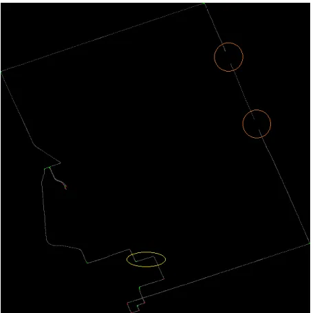
Figure 4.8 for driver 2 shows the same set of results as Figure 4.7 for driver 1. The PBTD algorithm detected two false positives for driver 3, shown in Figure 4.9. Note that there are two turns in the yellow circle in Figure 4.9 that occur close together.
4.3. Results andDiscussion 27
Table 4.4 shows the raw data frames where the second false positive was detected, which was shortly after the first FP. Again, the steering wheel position is large, this time to the right, and there is a change in direction as detected by Algorithm 2. Figure 4.11 also shows a map view of this FP and, again, it looks like a turn occurred.
Figure 4.9: Plotted route of driver 3 with 2 FP
Frame Number Latitude Longitude Speed Brake Pressure Gas Pressure Steering Wheel Position
37977 42.9947 -81.2116 7 1 0 60
37978 42.9947 -81.2117 7 1 0 54
. . .
38067 42.9947 -81.2117 12 1 0 -234
38068 42.9947 -81.2118 13 1 0 -237
Table 4.3: Raw data of driver 3 where the first false turn was detected
Driver 4 has correct results like drivers 1 and 2, except driver 4 turned from Waterloo Street to Pall Mall Street and Pall Mall Street to Richmond Street instead of Waterloo Street to Central Avenue and Central Avenue to Richmond Street (refer to Figure 4.12). This is the first instance of the driver deviating from the predetermined route. Turns detected for these deviations will be included in the analysis, as long as they do not occur in parking lots.
This is also the first instance of missing data. There are two occurances along Highbury Avenue where there is no GPS data. They did not affect the results for driver 4, however it will be shown later that missing data will not detect turns that occur during that time frame. This is one of the limitations of the PBTD algorithm.
28 Chapter4. Position-BasedTurnDetection
Frame Number Latitude Longitude Speed Brake Pressure Gas Pressure Steering Wheel Position
38247 42.9947 -81.2119 5 39 0 524
38248 42.9947 -81.212 5 38 0 524
. . .
38386 42.9947 -81.212 1 1 1 276
38387 42.9946 -81.2118 17 1 65 56
Table 4.4: Raw data of driver 3 where the second false turn was detected
Figure 4.10: Map view of driver 3 where the first false turn was detected
Figure 4.11: Map view of driver 3 where the second false turn was detected
4.3. Results andDiscussion 29
Figure 4.13: Plotted route of driver 5 Figure 4.14: Plotted route of driver 6
distortions, the results were not affected. However, turns that occurred where there was missing data were not detected. For example, the turns at Richmond Street and Sunningdale Road, and Sunningdale Road and Highbury Avenue were not detected. Since these turns were essentially missing due to GPS, they are not counted as true turns. So out of a total of 16 true turns for driver 5, 16 were detected by the algorithm.
In general, distorted GPS data will not have an affect on the analysis of turns, since the analysis only involves vehicle parameters during the turn; not latitude and longitude. Vehicle parame-ters will fluctuate within a turn which is why they are included in the analysis. Latitude and longitude, as discussed earlier, will only fluctuate by 0.0001, which is not useful for analysis. Hence they will be excluded, so distorted GPS data will not have an affect on the end results.
Figure 4.14 shows the route taken by driver 6. There are a few differences to highlight. First, there are a few parking lot turns along Sunningdale Road that were excluded. Second, driver 6 went from York Street to Richmond Street, which skipped the two turns from York Street to Talbot Street and Talbot Street to King Street. Lastly, there was missing data from Highbury Avenue to Dundas Street, so the algorithm was not able to detect this turn. Despite having three less true turns than the official route, all the turns were detected for driver 6.
30 Chapter4. Position-BasedTurnDetection
did not occur in a parking lot. In total, driver 7 has 17 true turns out of which 17 were detected by the algorithm.
Figure 4.15: Plotted route of driver 7 Figure 4.16: Plotted route of driver 8
Figure 4.16 shows distortions in GPS coordinates for driver 8. It is difficult to conclude if these distortions also caused some missing data, although it appears that if the coordinates were oriented properly, the cut-offends would meet. This is speculated by matching the distance along Sunningdale Road and Highbury Avenue in Figure 4.16 to the distance of those roads in Figure 4.15. Driver 8 also had a slight detour. After looking at the video sequences for driver 8, it appears that they missed the right turn from Highbury Avenue to Dundas Street and had to turn around by going into a parking lot. These parking lot turns were excluded, but the left turn from Highbury Avenue back onto Dundas Street was included. This caused driver 8 to have the same amount of turns as the official route, with the turn from Highbury Avenue to Dundas Street being a left turn instead of a right turn.
Figure 4.17 shows that there is missing data for driver 9. This caused the turn from Richmond Street to Oxford Street to go undetected, leaving 17 true turns for driver 9 of which 17 were detected.
4.3. Results andDiscussion 31
if the value of BEND T HRES HOLDwas changed to accommodate this turn, it would cause more false positives to be detected and hurt the accuracy of the algorithm.
Figure 4.17: Plotted route of driver 9 Figure 4.18: Plotted route of driver 10 with 1 FN
Frame Number Latitude Longitude Speed Brake Pressure Gas Pressure Steering Wheel Position
69822 42.9883 -81.2439 24 1 26 -152
69823 42.9884 -81.2438 24 1 26 -139
. . .
69851 42.9884 -81.2438 26 1 32 -33
69852 42.9885 -81.2438 26 1 32 -32
. . .
69881 42.9885 -81.2438 28 1 26 3
69882 42.9885 -81.2439 28 1 26 4
Table 4.5: Raw data of driver 10 where a turn should have been detected
The data for drivers 11 and 12 (see Figures 4.19 to 4.20) did not have any issues, except some missing data for driver 12 along Sunningdale Road. The official route was taken by these 2 drivers with no GPS distortions and all turn events were detected.
32 Chapter4. Position-BasedTurnDetection
Figure 4.19: Plotted route of driver 11 Figure 4.20: Plotted route of driver 12
view (shown in Figure 4.22) does not seem to indicate that a turn occurred, but perhaps a lane change.
Frame Number Latitude Longitude Speed Brake Pressure Gas Pressure Steering Wheel Position
76488 42.9910 -81.2482 12 46 0 -116
76489 42.9910 -81.2483 12 44 0 -120
. . .
76547 42.9910 -81.2483 11 1 33 -103
76548 42.9910 -81.2484 11 1 33 -100
Table 4.6: Raw data of driver 13 where a false turn was detected
Tables 4.7 and 4.8 show where the two missed turns should have been detected by the al-gorithm. Both tables show that the reason the turns were not detected as the same reason a turn was not detected for driver 10: the average steering wheel position was too small to
ex-ceedBEND T HRES HOLD. The average steering wheel position was -29.29 between frames
4.3. Results andDiscussion 33
Figure 4.21: Plotted route of driver 13 with 1 FP and 2 FN
Figure 4.22: Map view of driver 13 where a false turn was detected
Frame Number Latitude Longitude Speed Brake Pressure Gas Pressure Steering Wheel Position
63676 42.9807 -81.2507 15 1 27 -406
63677 42.9807 -81.2506 15 1 23 -399
. . .
63706 42.9807 -81.2506 18 1 0 -203
63707 42.9808 -81.2506 18 1 0 -200
. . .
63766 42.9808 -81.2506 9 93 0 10
63767 42.9809 -81.2506 9 93 0 10
. . .
64066 42.9809 -81.2506 14 1 39 3
64067 42.9810 -81.2507 14 1 39 3
34 Chapter4. Position-BasedTurnDetection
Frame Number Latitude Longitude Speed Brake Pressure Gas Pressure Steering Wheel Position
64726 42.9818 -81.2510 1 83 0 -129
64727 42.9818 -81.2511 1 83 0 -128
. . .
65506 42.9818 -81.2511 5 54 0 141
65507 42.9819 -81.2511 5 70 0 141
. . .
65747 42.9819 -81.2511 23 1 80 142
65748 42.9820 -81.2510 23 1 80 136
Table 4.8: Raw data of driver 13 where the second FN should have been detected
4.3. Results andDiscussion 35
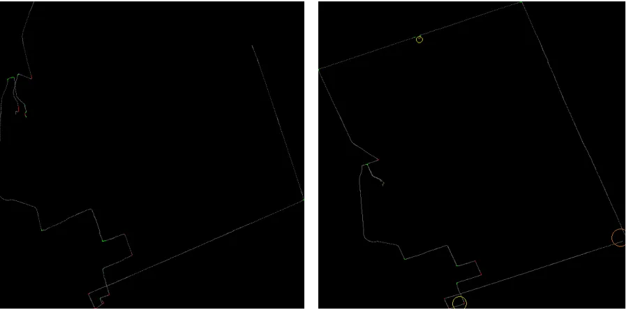
Figure 4.24: Plotted route of driver 15 Figure 4.25: Plotted route of driver 16
Drivers 14 and 15 (see Figures 4.23 and 4.24) did not have any issues. There was some missing data along Richmond Street for driver 14, but this did not have an affect on the results. In Figure 4.25 it is clear that there are large GPS distortions for driver 16. But, like with drivers 5 and 8, these distortions did not affect the accuracy of the algorithm.
Driver
1 2 3 4 5 6 7 8 9 10 11 12 13 14 15 16 Total True Turns 18 18 18 18 16 16 17 18 17 18 18 18 16 16 18 18 278
PBTD 18 18 20 18 16 16 17 18 17 17 18 18 15 16 18 18 278
FP 0 0 2 0 0 0 0 0 0 0 0 0 1 0 0 0 3
FN 0 0 0 0 0 0 0 0 0 1 0 0 2 0 0 0 3
36 Chapter4. Position-BasedTurnDetection
Using Equation 4.15 and the results summarized in Table 4.9, the accuracy of the PBTD algo-rithm can be determined:
A = nT −FPT −FNT
nT
(4.16) = 278−3−3
278 (4.17)
= 0.9784 (4.18)
= 97.84% (4.19)
Based on this equation, the algorithm achieves 97.84% accuracy.
There has been some debate over whether missed turns due to missing data, which has been seen with drivers 5, 6, 9 and 13, should be counted as true turns. From one perspective, these missing turns could argue that the PBTD algorithm should be modified to accommodate the possibility of missing data, or use a different method entirely that is able to impute when there is missing data. From another perspective, it is arguable that it is not the limitations of the algorithm but of the RoadLab dataset itself. In either case, Table 4.10 summarizes the results with missed turns due to missing data included. The accuracy of the algorithm then becomes 95.77%.
Driver
1 2 3 4 5 6 7 8 9 10 11 12 13 14 15 16 Total True Turns 18 18 18 18 18 17 17 18 18 18 18 18 18 16 18 18 284
PBTD 18 18 20 18 16 16 17 18 17 17 18 18 15 16 18 18 278
FP 0 0 2 0 0 0 0 0 0 0 0 0 1 0 0 0 3
FN 0 0 0 0 2 1 0 0 1 1 0 0 4 0 0 0 9
Table 4.10: Results of the Position-Based Turn Detection algorithm with missed turns (due to missing data) included as actual turns
An accuracy of 97.84% and 95.77% holds promise, however there are a couple areas that need to be considered to improve the algorithm in the future:
1. BEND T HRES HOLD,
2. FRAME T HRES HOLDand
3. Distortion of GPS data.
4.3. Results andDiscussion 37
bends and FRAME T HRES HOLD successfully removes duplicate turns. It is possible that the value of these thresholds may have overfitted the results for this specific route, especially
FRAME T HRES HOLD. FRAME T HRES HOLD assumed turns could not occur less than
11.3 seconds apart, which isn’t necessarily true of all routes. The algorithm is supposed to work optimally given any route, and it is difficult to prove that the value ofBEND T HRES HOLD
would work accordingly. Future research could focus on choosing thresholds independent of the route taken.
Chapter 5
Cluster Analysis
As the turn detection methods identified (fstart, fend) turn pairs, it also extracted information about the turn. Algorithms 2 and 3 calculated the average, standard deviation, kurtosis and skewness of:
1. speed,
2. brake pressure, 3. gas pressure, and 4. steering wheel position.
They also calculated the acceleration of each turn, which was defined as:
a= vfend −vfstart
d , (5.1)
wherevfend is the speed at the end of the turn andvfstart is the speed at the start of the turn. The duration,d, was defined in Equation 4.12. Duration is also used to analyze the time it takes to complete a turn. The last two descriptors are the age and gender of the driver, as they may be useful in categorizing driver behaviour.
Kurtosis and skewness are computed as metrics which, along with the average and standard deviation, become part of the set of descriptors for input to the clustering algorithm. These two metrics - kurtosis and skewness - will only be used as measures to characterize turns, while average and standard deviation will be used to analyze the cluster results.
The rest of the chapter is organized as follows. In the next section, all the preprocessing steps will be explained. In this section, normalization is performed on the data, and files are generated in order to analyze driving behaviour prior to a turn, during a turn, and after a turn. In Section 5.2, K-Means clustering is introduced and is performed on all preprocessed files generated from Section 5.1 using the most optimal value forK. Finally, in Section 5.3, cluster assignments are evaluated for consistency across pre-, during and post- turns. An optimal time
5.1. Preprocessing 39
will be selected before and after a turn that will be most suitable for cluster analysis in the future.
5.1
Preprocessing
In total, there are 20 descriptors for each turn. This research will analyze driving behaviour across all drivers by averaging all the turns of each driver into one set of descriptors. This will create one file for analysis with 16 entries representing each driver, where each entry contains the average of each of the 20 descriptors. The aim of this research is to analyze driver behaviour in relation to other drivers in order to build towards a computational model of driver behaviour. This is why all the turns are averaged for each driver instead of looking at turns within each driver, and then each driver is analyzed against one another.
Before the averaging takes place, the values of 18 descriptors need to be normalized (excluding age and gender) so that analysis is done on the same scale, which will prevent any of the descriptors from skewing the results. To do this, the MinMaxScaler method was used from the scikit-learn Python library to normalize all descriptor values for all drivers between 0 and 1. Steering wheel and acceleration are the only descriptors that can have negative values, so the following equation was used to extract the zero value after normalization:
zero value= −min
max−min, (5.2)
whereminis the lowest value for that descriptor andmaxis the highest value. Table 5.1 shows the zero values for the average, standard deviation, kurtosis and skewness of the steering wheel descriptor, as well as acceleration.
Zero value
Average of wheel position 0.42291678
Standard deviation of wheel position 0.5061441
Kurtosis of wheel position 0.12448418
Skewness of wheel position 0.32532348
Acceleration 0.3485342
Table 5.1: Zero values of steering wheel position and acceleration during turns
The raw RoadLab data was not normalized because it would reduce the capability of choosing an optimal value for BEND T HRES HOLD.