Paul Bottinelli1? and Joppe W. Bos2
1 EPFL, Lausanne, Switzerland 2
NXP Semiconductors, Leuven, Belgium
Abstract. Since the discovery of simple power attacks, the cryptographic research community has developed significantly more advanced attack methods. The idea behind most algorithms remains to perform a statistical analysis by correlating the power trace obtained when executing a cryptographic primitive to a key-dependent guess. With the advancements of cryptographic countermeasures, it is not uncommon that sophisticated (higher-order) power attacks require computation on many millions of power traces in order to find the desired correlation.
In this paper, we study the computational aspects of calculating the most widely used correlation coefficient: the Pearson product-moment correlation coefficient. We study various time-memory trade-off techniques which apply specifically to the cryptologic setting and present methods to extend already completed computations using incremental versions. Moreover, we show how this technique can be applied to second-order attacks, reducing the attack cost significantly when adding new traces to an existing dataset. We also present methods which allow one to split the potentially huge trace set into smaller, more manageable chunks in order to reduce the memory requirements. Our concurrent implementation of these techniques highlights the benefits of this approach as it allows efficient computations on power measurements consisting of hundreds of gigabytes on a single modern workstation.
Keywords:Side-channel analysis, CPA, Pearson correlation coefficient, higher-order attacks.
1 Introduction
Since the late 1990s it is publicly known that the (statistical) analysis of a power trace obtained when executing a cryptographic primitive might correlate to, and hence reveal information about, the secret key material used [13]. This active research area has seen a lot of development over the years: from successfully retrieving the secret key material by inspecting a single power trace using simple power analysis through differential power analysis [13] to using several time samples [17, 29, 11] (cf. [14] for a survey on this topic). Eventually this led to the more general correlation power analysis [6] which might need to inspect a large amount of traces in order to reveal correlations between the power consumption and the bits of the secret key. Moreover, the complexity of the attacks used have increased to higher (nth) order analysis [17]. In this
setting one computes joint statistical properties of the power consumption of n samples in order to try and deduce information about the bits of the secret key material used.
This has led to a significant increase in the number of correlation coefficients one has to compute. Researchers have reported handling millions [20, 24, 19], ten million [4], a hundred million [21] and up to three hundred million power traces [3]. This increase of available data requires more processing power in order to compute the required statistical analysis. This is illustrated by recent work: e.g. [1, 18] investigates the usage of graphics processing units to accelerate the computation while [16] explores the sophisticated usage of high-performance computing in this setting. Although many hardware designers and power analysis experts
?This work was done while the first author was an intern in the innovation center crypto & security at NXP
report whether the implementations of their techniques withstand (higher-order) correlation attacks, it is often not reported how much time was required to mount such attacks.
Over the last decade correlation power analysis (CPA) has become widely used and pre-ferred over differential power analysis since it performs better and requires fewer traces [5]: both important characteristics for measuring the effectiveness of an attack. One of the main ingredients in algorithms based on CPA is the computation of the correlation coefficient. In this paper we take a closer look at the Pearson product-moment correlation coefficient [23], simply referred to as Pearson’sρ, from a computational point of view, taking its role in cryp-tology into account. Although other correlation coefficients have been considered as well (e.g. in [2]), Pearson’sρhas been used in almost all correlation power attacks over the last decade, since it allows for an efficient correlation computation.
There are a lot of time-memory trade-off techniques one can apply to reduce the compu-tational cost of Pearson’s ρ in the cryptologic setting. We study some of these techniques in detail and explore the available optimization options when computing correlations in the set-ting of higher-order attacks. Additionally, we investigate the setset-ting where additional traces are added after an initial CPA attack did not reveal any leakage and we present algorithms which can re-use computations in both the first and second order setting. This study of com-putational aspects is complemented with techniques allowing the computation of Pearson’s ρ on memory constrained devices or, viewed differently, to compute the correlation function on huge data sets using conventional desktop machines. We demonstrate the effectiveness of our approach by showing implementation results of the methods used.
2 Preliminaries
Let X, Y be random variables with values uniformly distributed over R, let xi, yi, where 1≤i≤n, be nsamples of these variables, respectively. In this setting the expected value is denoted asE[X] = ¯x= n1Pn
i=1xi, the covariance asσ(X, Y) =E[(X−E[X])(Y −E[Y])] =
E[XY]−E[X]E[Y], the variance as Var(X) =σ(X, X) =σ2
X =E[(X−E[X])2] =E[X2]− E[X]2 = 1
n
Pn
i=1(xi−x)¯ 2=
1
n
Pn
i=1x2i
−x¯2, and the standard deviation asσ
X =
p
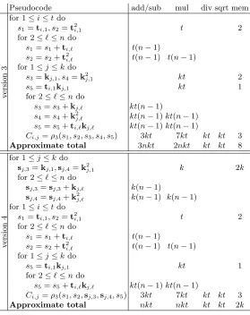
Table 1.Three different strategies to compute Ci,j =ρ(Ti,Kj) for all 1≤i≤t, 1≤j≤k as is common
in first order CPA. The three versions increasingly use the time-memory trade-off paradigm. The memory requirement in parentheses for version 2 is in the case where the input cannot be overwritten.
Pseudocode add/sub mul div sqrt mem
v
e
rsion
0
for 1≤i≤tdo ¯
t= mean(Ti) t(n−1) t 1
for 1≤j≤k do ¯
k= mean(Kj) kt(n−1) kt 1
Ci,j=ρ1(Ti,¯t,Kj,k¯) kt(5n−3)kt(3n+ 1) kt kt 6
Approximate total 6nkt 3nkt 2kt kt 8
v
e
rsion
1
for 1≤i≤kdo ¯ki= mean(Ki) k(n−1) k k
for 1≤i≤tdo ¯
t= mean(Ti) t(n−1) t 1
for 1≤j≤k do
Ci,j=ρ1(Ti,¯t,Kj,k¯j) kt(5n−3)kt(3n+ 1) kt kt 6
Approximate total 5nkt 3nkt kt kt k
v
e
rsion
2
for 1≤i≤kdo ¯
ki= mean(Ki), ˆki= 0 k(n-1) k k
for 1≤j≤ndo
ki,j=ki,j−¯ki kn (kn)
ˆ
ki= ˆki+k2i,j kn kn k
for 1≤i≤tdo ¯
t= mean(Ti) t(n−1) t 1
for 1≤j≤k do
Ci,j=ρ2(Kj,ˆkj,Ti,¯t) kt(3n−2)kt(2n+ 1) kt kt 4
Approximate total 3nkt 2nkt kt kt 2k
(kn)
A power trace denotes the power consumption of the device at t points in time during a cryptographic operation. The adversary usually monitors a large amount of such traces in order to cancel the effect of the noise δ. Typically this is done while setting k to a single byte of the key in order to limit the number of enumerations to 28 = 256. As an example,
when targeting the Advanced Encryption Standard [8] (AES) it is common to target the intermediate state after the S-box of the first round in the Hamming weight model. Hence, given a plain-text byte p one computes the estimated power consumption of 28 key guesses
as PM(S(p⊕i)) where the power model function PM computes the Hamming weight, the functionS is the AES S-box and 0≤i <28.
More specifically, letT be a measurement consisting ofntraces where each trace recorded data at t different time points: hence, T consist of elements ti,j ∈ R for 1 ≤ i ≤ t and
1≤ j ≤ n. WithTi we denote a finite sequence of lengthn, Ti = [ti,1,ti,2, . . . ,ti,n], which consists of a single measurement of each trace sampled at time point i. Similarly, we define the matrixK of k estimated power consumption of key guesses consisting of valueski,j ∈R
with 1≤i≤k and 1≤j≤ncorresponding to thesen traces.
T = T1 T2 .. . Tt =
t1,1t1,2 . . .t1,n
t2,1t2,2 . . .t2,n ..
. ... . .. ...
tt,1 tt,2 . . .tt,n
, K =
K1 K2 .. . Kk =
k1,1 k1,2. . .k1,n
k2,1 k2,2. . .k2,n ..
. ... . .. ...
kk,1kk,2. . .kk,n
3 Pearson’s ρ and Time-Memory Trade-Off Techniques
The Pearson product-moment correlation coefficient, or simply Pearsonρ[23], is a well-known method to measure the linear dependence between two random variables. This correlation is measured as a value between−1 (total negative correlation) and +1 (total positive correlation) where a value of zero indicates no correlation. The formula for this correlation is
ρ(X, Y) = σ(X, Y) σXσY
= E[(X−x)(Y¯ −y)]¯ σXσY
, (2)
and can be computed, using the notation from Section 2, as
ρ(X, Y) =
Pn
i=1(xi−x)(yi¯ −y)¯ pPn
i=1(xi−x)¯ 2pPni=1(yi−y)¯ 2
. (3)
There are various strategies to compute Eq. (3). In statistics, the typical setting is to computeρ(X, Y) once or possibly compute multiple correlation coefficients where every com-putation involves different datasetsXandY. In the setting of CPA, this situation is different: one wants to correlate the n trace-values at a fixed point in time with the k different key-guesses (consisting of a vector of n elements each). Hence, one computes the k correlation coefficients where one of the inputs toρ is fixed. This allows one to perform precomputations in order to lower the number of arithmetic operations (at the cost of additional memory).
In Table 1 we outline three approaches based on the time-memory trade-off paradigm. We assume that, as is the case when performing a first order CPA, we want to compute t·k correlations asCi,j =ρ(Ti,Kj) for all 1≤i≤t, 1≤j≤k. Table 1 states the computational costs, expressed in terms of additions/subtractions, multiplications, divisions and square root computations required. The approximate total only shows the accumulated part of the largest terms where we assume thatn > t > k (which is typical for CPA).
Version 0 uses no additional memory. For efficiency reasons the means of the Ti are computed once before entering the second for-loop and re-used. The ρ1 function is identical
to Eq. (3) with the means precomputed
ρ1(T,¯t,K,k) =¯
Pn
i=1(ti−t)(¯ ki−k)¯
q Pn
i=1(ti−¯t)2
q Pn
i=1(ki−¯k)2 .
Version 1 precomputes the means of thekdifferent keys, significantly reducing the number of loads from memory and the number of addition and divisions. When k = 28, a common
choice when targeting an individual byte of the secret key, this is a cheap way, in terms of memory, to gain performance. Compared to version 0, the number of additions in the most significant term has been reduced by nktand we only need to compute half of the divisions.
Version 2 extends the precomputations and computes both (xi −x) and¯ Pn
i=1(xi−x)¯ 2
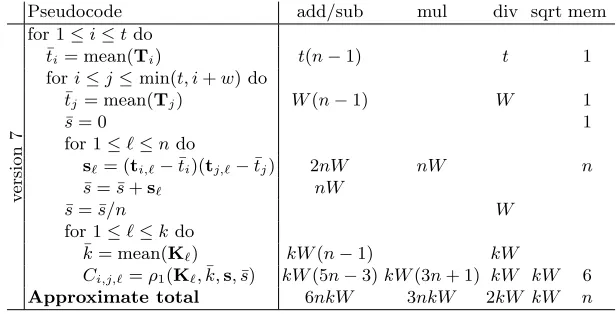
Table 2.Two different strategies to compute Ci,j = ρ(Ti,Kj) for all 1 ≤i ≤t, 1 ≤ j ≤ k based on the
incremental correlation formula (see Eq. (4)) and exploiting the time-memory trade-off paradigm.
Pseudocode add/sub mul div sqrt mem
v
ersion
3
for 1≤i≤tdo
s1=ti,1, s2=t2i,1 t 2
for 2≤`≤ndo
s1=s1+ti,` t(n−1)
s2=s2+t2
i,` t(n−1) t(n−1)
for 1≤j≤kdo
s3=kj,1, s4=k2j,1 kt 2
s5=ti,1kj,1 kt 1
for 2≤`≤ndo
s3=s3+kj,` kt(n−1)
s4=s4+k2j,` kt(n−1)kt(n−1)
s5=s5+ti,`kj,` kt(n−1)kt(n−1)
Ci,j=ρ3(s1, s2, s3, s4, s5) 3kt 7kt kt kt 3
Approximate total 3nkt 2nkt kt kt 8
v
ersion
4
for 1≤j≤kdo
sj,3=kj,1,sj,4=k2j,1 k 2k
for 2≤`≤ndo
sj,3=sj,3+kj,` k(n−1)
sj,4=sj,4+kj,`2 k(n−1) k(n−1)
for 1≤i≤tdo
s1=ti,1, s2=t2i,1 t 2
for 2≤`≤ndo
s1=s1+ti,` t(n−1)
s2=s2+t2i,` t(n−1) t(n−1)
for 1≤j≤kdo
s5=ti,1kj,1 kt 1
for 2≤`≤ndo
s5=s5+ti,`kj,` kt(n−1)kt(n−1)
Ci,j=ρ3(s1, s2,sj,3,sj,4, s5) 3kt 7kt kt kt 3
Approximate total nkt nkt kt kt 2k
multiplications). When overwriting existing memory xi with xi −x¯ the Pearson ρ can be computed as
ρ2(X,x, Y,ˆ y) =¯ Pn
i=1xi·(yi−y)¯
p
ˆ x·Pn
i=1(yi−y)¯ 2
.
4 Incremental Pearson
It is well-known that Eq. (3) can be rewritten as
ρ(X, Y) = n
Pn
i=1xiyi− Pn
i=1xi Pn
i=1yi q
nPn
i=1x2i −(
Pn
i=1xi) 2q
nPn
i=1yi2−(
Pn
i=1yi)
2 (4)
by computing the means directly (substituting ¯x with n1Pn
i=1xi) and performing some
re-ordering. This alternative formula allows for different precomputation strategies and, more-over, has additional benefits which are discussed in this section.
4) discussed here and which compute Eq. (4) are summarized in Table 2. This approach essentially needs to compute the five values
s1 =
n
X
i=1
xi, s2 =
n
X
i=1
x2i, s3 =
n
X
i=1
yi, s4 =
n
X
i=1
yi2, s5 =
n
X
i=1
xiyi.
Once these have been computed Eq. (4) can be computed as
ρ3(s1, s2, s3, s4, s5) =
(ns5−s1s3) p
(ns2−s21)(ns4−s23)
.
Version 3 in Table 2 computes ρ3 without using additional storage where ti,j acts as the xi and ki,j as yi. For a fixed Ti the values of s1 and s2 are computed at the beginning
of the for-loop and re-used for the multiple key guesses. However, the values s3, s4 and
s5 are recomputed. Version 4 also pre-computes s3 and s4 at the cost of storing 2k
data-elements. This reduces the number of required additions by a factor three to nkt and the number of multiplications by a factor two to nkt. It does not make sense to also pre-compute s5 =Pni=1xiyi since these results cannot be re-used; this would only costs additional storage without reducing the number of arithmetic operations.
Incremental first-order CPA. In addition to being computationally more efficient than
the fastest “standard version” variant (cf. the performance data of version 2 in the left plot of Figure 4) Eq. (4) has another interesting feature. Suppose we perform a CPA attack on a trace set of sizen, but are not able to observe any significant leakage. In the hope of observing some leakage, an adversary could try and add m additional traces to the measurement. By using any variant of the “standard version” (version 0, version 1, or version 2), the attacker must first perform his attack on the set of ntraces, then on the larger set containingn+m traces, duplicating many arithmetic computations. Using a variation of version 4, the adversary can compute the correlations on the first trace set, but then extend the computations to compute a CPA on the extended set ofn+m traces without using a significant amount of additional memory. Indeed, Eq. (4) only requires to compute sums of elements of vectors, which can be stored and later updated by adding the elements of the new traces. This approach is infeasible using, for instance, version 2.
Let us consider two variants of version 4. In version 5, the 2t values si,1 = Pni=1xi and
si,2 =Pni=1x2i are precomputed and reused when adding more traces. Similarly, we extend version 5 to a version 6 where we also precompute and reuse the tk values si,5 =Pni=1xiyi.
Then the cost of computing the correlation coefficients using ntraces first and subsequently withm+ntraces is summarized in the following table where only the largest terms are shown.
version 2 version 5 version 6
Approximate #add 3kt(2n+m) kt(2n+m) kt(m+n)
Approximate #mul 2kt(2n+m) kt(2n+m) kt(n+m)
Approximate #mem kn 2(k+t) kt
of multiplications by a factor two to 3ktn(compared to version 2). If one can spare to store kt data elements the cost of version 2 is even further reduced: the number of additions by a factor 4.5 to 2ktn and the number of multiplications with a factor three to 2ktn. Although these are only constant improvements, they can make a significant difference in practice when computing CPA on large datasets where botht andn can be very large.
5 Computational Aspects of Second Order CPA
A common measure to protect against side-channel attacks is known as masking (see e.g. [7, 10, 26]) where the secret data is split into multiple shares. One approach to attack such schemes is to combine these shares in order to find a correlation between the power consumption of the combination of these shares and the secret material: this is known as higher-order power analy-sis (see e.g. [17, 29, 11]). In order to combine two power measurementsT1 = [t1,1,t1,2, . . . ,t1,n]
and T2 = [t2,1,t2,2, . . . ,t2,n] as C(T1,T2) = [t1,t2, . . . ,tn] one can compute the normalized product (computeti= (t1,i−T¯1)(t2,i−T¯2) for 1≤i≤n) [7], the absolute difference
(com-puteti =|t1,i−t2,i|for 1≤i≤n) [17] or the sum (computeti =t1,i+t2,ifor 1≤i≤n) [28]. As shown in [25, 28] the normalized product approach performs best when Pearson’s corre-lation coefficient is used and assuming the Hamming weight leakage model. Following these conclusions we focus exclusively on this combining function in this section in the setting of second order CPA.
Assuming that we also consider the combination of a power measurement with itself, there are in totalPt
i=1i=t(t+ 1)/2 possible unique pairs from the t power measurements.
In practice, however, one does not necessarily combine all possible pairs. The computation of the shares usually occurs within a bounded time span. Therefore we introduce another parameter when computing higher order attacks, the window sizew. This positive integer is an estimation of the maximum distance between two shares. In the algorithms considered in this section, given a window sizew≤t and tpower measurements,
W =W(t, w) = (t−w)w+ w
X
i=1
i=w(t−w−1
2 )
denotes the number of pairs considered. The smaller the window w, the fewer computations one has to perform; note that settingw=tis equivalent to computing on all possible pairs. In the following, similar to the analysis in Sections 3 and 4, we describe three basic algorithms to perform second-order CPA and list various time-memory trade-off techniques that can be applied. We exclusively focus on optimizations improving the most significant term in the computational cost and do not consider various minor optimizations one can achieve as well.
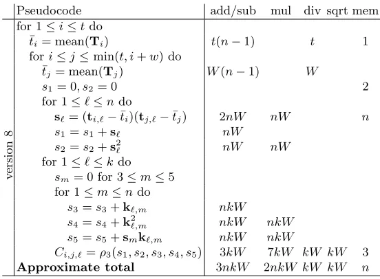
5.1 Naive Second Order CPA: Version 7
Table 3 outlines the “naive” version of a second-order CPA. This version does not use any auxiliary memory except one vector of n elements which holds the result of the combining function C(T1,T2). Following the approach from Section 3 one can reduce the number of
arithmetic operations at the cost of using additional memory by 1. subtracting mean ¯sfrom the s` “in-place” fornW subtractions,
Table 3.Second order CPA with windowwand normalized product combining based on Eq. (2).
Pseudocode add/sub mul div sqrt mem
v
ersion
7
for 1≤i≤tdo ¯
ti= mean(Ti) t(n−1) t 1
fori≤j≤min(t, i+w) do ¯
tj= mean(Tj) W(n−1) W 1
¯
s= 0 1
for 1≤`≤ndo
s`= (ti,`−t¯i)(tj,`−t¯j) 2nW nW n
¯
s= ¯s+s` nW
¯
s= ¯s/n W
for 1≤`≤kdo ¯
k= mean(K`) kW(n−1) kW
Ci,j,`=ρ1(K`,¯k,s,s¯) kW(5n−3)kW(3n+ 1) kW kW 6
Approximate total 6nkW 3nkW 2kW kW n
3. precomputing thekmeans ofKi, at a cost of approximatelyknadditions andkdivisions, 4. precomputing theksums of balanced squares ofKi, at a cost of an additionalknadditions,
knsubtractions and knmultiplications,
5. if the input can be overwritten, replace the ki,j by ki,j − ¯ki, otherwise store the nk normalized ki,j values,
By using optimizations 1 and 2, we obtain a first variant of version 7 (denoted version 7a) which does not require additional memory but allows us to savenkW additions, subtractions and multiplications, effectively reducing the number of additions and multiplications both by a factor 1.5.
By also applying optimizations 3 and 4, we obtain a second variant of version 7 (de-noted version 7b) which requires a medium amount of memory: this version precomputes 2k additional values which significantly reduces the computational cost, reducing the num-ber of addition and subtractions by a factor two (from 4nkW to 2nkW) and the number of multiplications by a factor two (from 2nkW tonkW).
Furthermore, by also applying optimization 5, we obtain the fastest version (denoted version 7c). This might come at no additional cost in terms of memory if the input can be overwritten or, if this is not an option, requires storage for nk additional values. This final trade-off allows us to save another nkW subtractions: a factor two improvement over version 7b.
5.2 Naive Second Order CPA using Eq. (4): Version 8
This version of a second order CPA modifies version 7 such that it uses Eq. (4) to compute the individual correlation coefficients; it is outlined in Table 4. Using this approach, we can directly benefit from the computation of the temporary vector s = C(T1,T2) to precompute some
values required in Eq. (4) with almost no additional computational cost. Analogue to version 7, the version presented in Table 4 requires almost no additional memory with the exception of what is needed to store the temporary vectors. One additional optimization improving the most significant term can be applied based on the time-memory trade-off paradigm
Table 4.Second-order CPA with windowwand normalized product combining based on Eq. (4)
Pseudocode add/sub mul div sqrt mem
v
e
rsion
8
for 1≤i≤tdo ¯
ti= mean(Ti) t(n−1) t 1
fori≤j≤min(t, i+w) do ¯
tj= mean(Tj) W(n−1) W
s1= 0, s2= 0 2
for 1≤`≤ndo
s`= (ti,`−¯ti)(tj,`−¯tj) 2nW nW n
s1=s1+s` nW
s2=s2+s2
` nW nW
for 1≤`≤kdo
sm= 0 for 3≤m≤5
for 1≤m≤ndo
s3=s3+k`,m nkW
s4=s4+k2`,m nkW nkW
s5=s5+smk`,m nkW nkW
Ci,j,`=ρ3(s1, s2, s3, s4, s5) 3kW 7kW kW kW 3
Approximate total 3nkW 2nkW kW kW n
By applying this single optimization, we can improve the computational cost of version 8 at the price of 2kadditional memory (denoted by version 8a). This version halves the number of multiplication (from 2nkW tonkW) and reduces the number of additions by a factor three (from 3nkW tonkW).
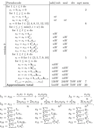
5.3 Incremental Second Order CPA: Version 9
The techniques used in Section 4 can also be applied to higher-order CPAs. In this section we outline how to achieve this in the second order CPA setting. Using such a version enables one to compute a second order CPAincrementally, resulting in potentially significant savings when adding more power traces to a power measurement. Obviously, the number of intermediate results one needs to keep track of increases in this setting. Instead of the five values in Section 4, one has to store thirteen in this case.
In order to deduce a formula based on these thirteen values, which can be updated incre-mentally, we replace the variable X with C(T, U): the combination of the two traces T and U. More precisely, given our choice of combining function, we replace the individual xi with (ti−¯t)(ui−u).¯
ρ(C(T, U), Y) = p nλ1−λ2s3
nλ3−λ22 p
ns9−s23
=ρ4(s1, . . . , s13) (5)
Table 5.Second-order CPA with window wand normalized product combining based on Eq. (5). Note that the operation count forρ4is an upper bound. This count can be reduced by simplifying Eq. (5). However, this does not reflect on the most significant term.
Pseudocode add/sub mul div sqrt mem
v
e
rsion
9
for 1≤i≤tdo
s1= 0, s6= 0 2
for 1≤j≤ndo
s1=s1+ti,j nt
s6=s6+t2i,j nt nt
sl= 0 forl∈ {2,4,8,11,12,13} 6
fori≤j≤min(t, i+w) do for 1≤`≤ndo
s2=s2+tj,` nW
s8=s8+t2j,` nW nW
s4=s4+ti,`tj,` nW nW
s12=s12+t2i,`tj,` nW nW
s13=s13+ti,`t2j,` nW nW
s11=s11+t2i,`t
2
j,` nW nW
for 1≤`≤kdo
sl= 0 forl∈ {3,5,7,9,10} 5
for 1≤m≤ndo
s3=s3+k`,m nkW
s9=s9+k2`,m nkW nkW
s5=s5+ti,mk`,m nkW nkW
s7=s7+tj,mk`,m nkW nkW
s10=s10+ti,mtj,mk`,m nkW nkW
Ci,j,`=ρ5(s1, . . . , s13) 13kW 24kW 7kW kW 7
Approximate total 5nkW 4nkW 7kW kW 20
λ1=s10−
s1s7+s2s5
n +
s1s2s3
n2 , λ2 =s4−
s1s2
n , λ3=s11−
2s2s12+ 2s1s13
n +
s2
2s6+ 4s1s2s4+s21s8
n2 −
3(s1s2)2
n3 ,
s1=Pni=1ti, s2=Pni=1ui, s3 =Pni=1yi,
s4=Pni=1tiui, s5=Pin=1tiyi, s6 =Pni=1t2i, s7=Pni=1uiyi, s8=Pin=1u2i, s9 =Pni=1y2i, s10=Pni=1tiuiyi, s11=Pni=1t2iu2i, s12=Pni=1t2iui, s13=Pni=1tiu2i.
Table 5 outlines the approach to implement Eq. (5) with some straightforward improvements, where the ti,m acts as theti, the tj,m acts as theui and thek`,m asyi. Again, we can reduce the number of operations by using more memory. We distinguish the following optimizations 1. precompute the 2k values s3 =Pni=1yi and s9 =Pni=1y2i, which requires approximately
2knadditions and kn multiplications.
2. precompute the kt values s5 = Pni=1tiyi. This precomputation requires approximately
ktnadditions and ktnmultiplications,
3. store the n products ti,`tj,` for all 1 ≤ ` ≤ n when computing them, which does not require any additional arithmetic operation.
A faster variant of version 9 can be obtained by applying optimization 1 (denoted version 9a) for an additional storage cost of 2k values. This optimization reduces the number of additions by a factor 53 from 5nkW to 3nkW and the number of multiplications by a factor
4
By also including optimization 2 (denoted version 9b) we apply the time-memory trade-off even further, requiring to store tk additional elements. The effect is significant, as not only the values5 is no longer computed in the innermost loop, but the values7 now comes for free.
Thus, in comparison to version 9, the number of additions is reduced to kn(t+W) (which for large values of W means a reduction by a factor five) while the number of multiplications is reduced to kn(t+ 2W) (which for large values ofW means a reduction by a factor two).
Finally, by also applying optimization 3, we obtain version 9c which saves nkW more multiplications for a cost ofnmemory, since only one multiplication has now to be computed in the innermost loop.
An overview of the cost of the various second order algorithms is given below. Approx. #add Approx. #mul Approx. #mem
Version 7 6nkW 3nkW n
Version 7a 4nkW 2nkW n
Version 7b 2nkW nkW n
Version 7c nkW nkW n or nk
Version 8 3nkW 2nkW n
Version 8a nkW nkW n
Version 9 5nkW 4nkW 14
Version 9a 3nkW 3nkW 2k
Version 9b nk(t+W) nk(t+ 2W) kt
Version 9c nk(t+W) nk(t+W) n
Incremental Second Order CPA. As stated in Section 5.3, version 9 has the potential
to reuse computations when adding more power traces to the power measurement. Indeed, keeping track of a few values allows for a much more efficient computation of the correlation coefficients when adding a batch of new traces to the power measurement. We consider the setting similar to the one in Section 4: the attacker first performs a second order CPA on a set of n traces. Next, an additional m traces are added to the power measurement and a computation on all the m+n traces is performed. Let us consider a variant of version 9 (denoted version 9d) consisting of an extension of version 9c in which we also store: the kW values
s10,i,j,` = m+n
X
a=1
ti,atj,ak`,a, for 1≤i≤t, i≤j≤min(t, i+w), and 1≤`≤k,
the 2tvalues
s2,i= n
X
j=1
ti,j ands8,i= n
X
j=1
t2i,j for 1≤i≤t,
and the 4W values
s4,i,j = n
X
`=1
ti,`tj,`, s11,i,j= n
X
`=1
t2i,`t2j,`, s12,i,j= n
X
`=1
t2i,`tj,`,
s13,i,j = n
X
`=1
ti,`t2j,`, for 1≤i≤tand i≤j ≤min(t, i+w).
version 7c version 8a version 9c version 9d Approx. #add kW(2n+m) kW(2n+m) k(t+W)(2n+m) k(t+W)(n+m) Approx. #mul kW(2n+m) kW(2n+m) k(t+W)(2n+m) k(t+W)(n+m)
Approx. #mem k(n+m) n+m n+m max(kW, n, m)
Considering a scenario where m=n, i.e. in which an attacker addsnnew traces to a set ofntraces (working with 2ntraces in total), version 7c requires 3nkW additions and 3nkW multiplications, and requires memory for 2kn elements, as the values cannot be modified in-place just as in the first order setting. Using much less memory, version 8a can compute this second order CPA with the same number of arithmetic operations but with much less memory. Version 9c slightly increases the computational cost of version 8a. Finally, version 9d reduces the number of additions and multiplications by a factor 1.5 with respect to version 9c. This comes at the cost of usingkW + 2t+ 4W more memory than version 9c. However, in practice, this might still be smaller than norm (since typically k= 28 and t≈103 while
n≈m >107).
6 Memory Constrained CPA
Reducing the computation time when computing the correlation coefficient is just one impor-tant characteristic in a state-of-the-art CPA implementation. Due to the common practice of collecting a large number of samples per trace (the variablet) and collecting a large number of traces (the variable n), values around n ≈ 108 are not uncommon [21, 3], the size of the
main memory available in common desktop machines is in most cases insufficient to load the entire measurement at once. In this section, we present some methods to efficiently partition the data under such memory constraints. These methods allow to perform CPA attacks on a large set of power traces on widely available desktop machines and do not significantly increase the computation time (in terms of number of arithmetic operations) compared to the setting where sufficient memory would be available.
6.1 Split across the Time Samples
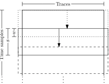
The most natural, and straightforward, way of reducing the memory requirement is to split the measurement across the time samples. The idea is to consider the entire set of traces at once but for a reduced number of time samples at a time. Consider the set of power traces as the matrix T (see the definition from Section 2) consisting ofn power traces, each of which consists oft power measurements. Lets < t be the number of time samples such that s×n elements in the trace file can be loaded into the main memory. When splitting across the time samples, one could loadssamples at a time, compute the correlation, then move to the next ssamples, and repeat the process until all correlations have been computed.
Time
sam
p
les
Traces
w
··
· ··· ··· ···
s
Fig. 1.A sliding window approach when splitting the data across the time samples.
s−w, can still read the entire window, until the s-th sample, into memory. After having computed the correlation coefficient of these w(s−w) combinations with the key guesses, the first (s−w) time samples are discarded, the last w samples are moved to the beginning and the next batch of (s−w) samples for all n traces are read until we have covered all t measurements. This approach is illustrated in Figure 1.
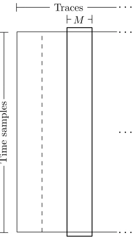
6.2 Split across the Traces
Another approach to partition the measurement in order to reduce the memory requirement, is to use a limited number of traces at a time but consider the entire range of time samples. One example of such a partitioning was already discussed in Section 4 and Section 5.3 in the setting of the incremental versions for computing Pearson’s correlation coefficient. This approach is illustrated in Figure 2. In this subsection we show how this partitioning can be conducted using the work by Dunlap [9] where it is studied how to combine correlation coefficients from different sets given the means, standard deviation and correlation of these sets.
This approach does not update the value of the correlation coefficient continuously, by adding new traces, but instead computes the correlation coefficient of a set consisting of fewer traces and combines these results to compute the (estimation of the) correlation coefficient when taking all traces into account. This approach also reduces the memory requirement significantly since a much smaller set of traces needs to be kept in memory at a time. Note that in this case, as we have access to the entire range of time samples, we do not need to use the sliding window approach presented in the previous section. Let
T=
t1
t2
.. .
tn
and K=
k1
k2
.. .
kn
be two vectors that we want to correlate in a correlation power analysis attack.Trepresents a vector from the matrixT at a fixed time point andKdenotes a vector from the matrix of estimated power consumptionK for a given key guess (as defined in Eq. (1)).
We then split the vectorT into m groups Mj having respective sizessj. Hence we have
Pm
Time
sam
p
les
Traces
M
··
·
··
·
··
·
··
·
Fig. 2.Loading the entire range of time samples into memory while processing a batch of traces at-a-time.
sizes of the groups Mj and Lj are equal, for all 1 ≤ j ≤m. Now, for each group of traces
Mj, we compute the m standard deviations σMj, the m means ¯Mj and the m correlation
coefficients with the corresponding groups from K, r(Mj,Lj). The same is done for the m standard deviationsσLj and them means ¯Lj.
In the following we present formulas which compute directly the final correlation given these values. Note, however, that in an actual implementation, the individual values should be combined incrementally to save on storage. The sizes sj of the groups of traces Mj and
Lj are selected such that the sj ·t+sj ·kmeasurement values fit into memory.
In [9], Dunlap present the following result, which we summarize in our setting, to compute the correlation coefficient of the larger trace set based on the mean, standard deviation and correlation coefficients of the smaller sets
ρ(T,K) =
Pm
i=1si
σMiσLiρ(Mi,Li) + ˜MiL˜i
r
Pm i=1si
σ2
Mi+ ˜M
2
i
r Pm
i=1si
σ2
Li+ ˜L
2
i
. (6)
We refer to this approach as exact combining. The ˜Mi (˜Li) are defined as the difference between the mean of the measurements of an individual time sample in ¯Mi (¯Li) and the mean of all the measurements of this time sample inT (K); i.e.
˜
Mi = ¯Mi−
Pm
j=1sjM¯j
Pm
j=1sj
, L˜i = ¯Li−
Pm
j=1sjL¯j
Pm
j=1sj .
Note that Eq. (6) computesexactly the same correlation coefficient as if directly computing on the larger trace files using Eq. (3) and is not an approximation.
Time
sam
p
les
Traces
··
·
··
·
··
·
· · ·
· · ·
· · ·
Fig. 3.Combining the approach from Fig. 2 and Fig. 1 intoblock-partitioning. Load part of the range of time samples using part of the traces at-a-time.
equaland the means of the smaller groups of key guesses Lj are equal then Eq. (6) can be simplified (cf. [9]) to
ρ(T,K) =
Pm
i=1σMiσLiρ(Mi,Li)
q Pm
i=1σM2 i
q Pm
i=1σ2Li
. (7)
We refer to this approach as approximate combining. Moreover, if one makes the assumptions that the standard deviations of all theMj are also equaland that all the standard deviations for all theLj are equal, then Eq. (7) simplifies further to
ρ(T,K) =m−1 m
X
i=1
ρ(Mi,Li). (8)
We refer to this approach as the arithmetic mean.
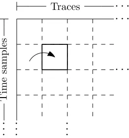
6.3 Block Partitioning
One can combine the approaches from Section 6.1 and Section 6.2. Using such a block-partitioning approach, we only consider a subset of the time samples and a subset of the traces. Then, similar to Section 6.1, we compute the correlation coefficients of these subsets, and store them in order to combine them with the correlation factors of the next chunks later. The combining of these correlation coefficients can be done following the approach from Dunlap presented in Section 6.2. This technique allows us to perform correlation attacks on very large data sets even when the available memory is limited. This approach is illustrated in Figure 3.
7 Benchmark Results and Experiments
0 10 20 30 40 50 60 70
1 2 3 4 5 6 7 8
Time (minutes)
Number of cores
version 0 version 1 version 2 version 3 version 4
20 40 60 80 100 120 140
1 2 3 4 5 6 7 8
Time (minutes)
Number of cores
version 7c version 8a version 9c
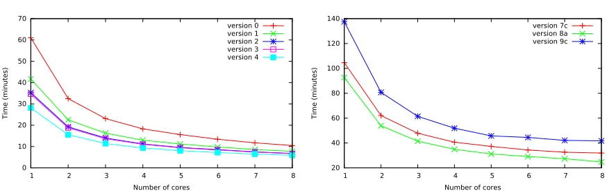
Fig. 4.Performance data when usingn= 107,k= 28, andt= 29. The left plot shows first-order CPA results computing 217 correlation coefficients while the plot on the right computes a second-order CPA usingw= 4
computing W(t, w)·256≈219 correlation coefficients. The reported timings include the loading time of the data from disk to memory.
file which needs to be loaded into memory is stored on a local 256 GB solid state disk (SSD) (Liteonit LCS-256M6S). As a reference we use a power measurement consisting of many time samples, from which we only use a smaller range oft= 29 samples, and wheren= 107 traces
have been collected. Each measurement is represented in an 8-byte double-precision point format. All intermediate computation performed are using double-precision floating-point arithmetic. All algorithms discussed in the previous sections can be made to compute the various correlation coefficients concurrently without too much overhead. By dividing the calculations in multiple threads we can reduce the computation time, taking advantage of the wide availability of multi-core machines.
7.1 First order CPA
In the left plot in Fig. 4 we show the performance results when using parametersn= 107,k=
28, andt= 29: i.e. computing 217 correlation coefficients using 107 traces. The correctness of
the implementation is verified with a slow (naive) single-threaded implementation of Pearson’s correlation coefficient. The left plot of Fig. 4 shows performance results when varying the number of cores used in the computation for the five different version. These performance numbers are in-line with the arithmetic counts from Table 1 and Table 2. The fastest “naive” version (version 2) performs almost identical compared to version 3. As expected from Table 2 version 4 performs best. These performance numbers include the time required to load the data from the SSD into memory which, on average, required 2.0 minutes. Hence, when ignoring the loading of the data, we observe a factor 1.9 speed-up when using two CPU cores, a factor 3.6 speed-up when using four CPU cores, and a factor 6.9 speed-up when using eight CPU cores compared to running on a single core considering version 4 of the algorithm.
7.2 Second order CPA
We also implemented the various approaches from Section 5. The right plot of Fig. 4 reports the performance results for the fastest variants of version 7, version 8, and version 9. Since all the data-types used are 8-byte double-precision floating points these tn= 29·107 values
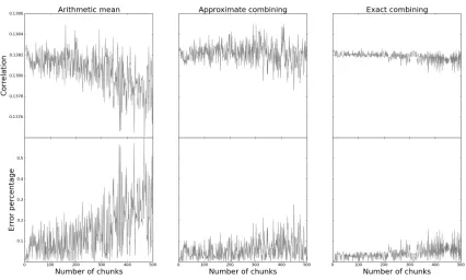
Fig. 5.Experimental results when computing the correlation coefficient using the arithmetic mean (Eq. (8)), approximate combining (Eq. (7)), and exact combining (Eq. (6)) approach. The number of chunksmis varied when using a total number of traces of 105. The top graphs show the computed correlation and the bottom graphs the error percentage to the real correlation coefficient.
data across the time samples (as outlined in Section 6.1) and load them in batches ofs= 64 time samples (which corresponds to batches of 4.9 GB). Extracting the correctstime samples of the power measurement file and loading this into memory requires 58 seconds per batch.
As expected from counting the number of required arithmetic instructions and memory requirement, version 8a performs the best among the considered variants which compute second order CPA, closely followed by version 7c. However, version 9c is considerably slower compared to the other two versions. Due to the relatively small windows size used (w = 4), version 9c computes a factor 1.25 more additions and multiplications compared to the two other versions, which explains the difference in terms of performance.
7.3 Combining using Dunlap’s approach
Figure 5 displays experimental results when applying the different combining approaches. For this experiment we used a (leaky) power measurement wheren= 105. We varied the number
be explained by the propagation of errors due to the finite precision which is used. Hence, in all three settings this allows us to split the number of traces in 200 chunks (each only holding 500 traces), compute the correlation coefficient on these smaller datasets and combine them such the result has an error less than 0.3 percent.
8 Conclusions and Future Work
Computing the Pearson product-moment correlation coefficient in the setting of (higher-order) correlation power attacks allows one to perform a number of precomputations which are not available in other (non-cryptologic) research areas. We have outlined different techniques to reduce the number of arithmetic operations and enable the attacker to add new traces incrementally without much computational overhead. Specifically, we have studied second-order attacks and demonstrated how they can be extended to the setting of adding traces on-the-fly. Furthermore, we have shown how one can compute on large datasets using commonly available computer architectures equipped with a modest amount of memory. In this latter setting we have used techniques from Dunlap [9] to combine the correlation coefficient from different small sets into the (estimate of the) correlation coefficient of the combination of these sets. Our benchmark and performance results show that the implementation of these techniques behave as expected and give a significant speed-up (both in performance and memory consumption).
A similar analysis can be performed on higher order correlation power attacks. An in-teresting exercise would be to derive incremental formulas for these higher order attacks, comparable to Eq. (4) for first order or Eq. (5) for second order, allowing to add traces on-the-fly. Similarly, it would be interesting to study the usage of different correlation coeffi-cient functions when computing (higher order) CPA and applying the time-memory trade-off paradigm. Examples include Spearman’s rank correlation coefficient [27] or Kendall’s rank correlation coefficient [12] (e.g. as applied in [2]).
References
1. T. Bartkewitz and K. Lemke-Rust. A high-performance implementation of differential power analysis on graphics cards. In E. Prouff, editor, CARDIS 2011, volume 7079 ofLecture Notes in Computer Science, pages 252–265. Springer, 2011.
2. L. Batina, B. Gierlichs, and K. Lemke-Rust. Comparative evaluation of rank correlation based DPA on an AES prototype chip. In T.-C. Wu, C.-L. Lei, V. Rijmen, and D.-T. Lee, editors,ISC 2008, volume 5222 ofLNCS, pages 341–354, Taipei, Taiwan, Sept. 15–18, 2008. Springer, Berlin, Germany.
3. B. Bilgin, B. Gierlichs, S. Nikova, V. Nikov, and V. Rijmen. Higher-order threshold implementations. In P. Sarkar and T. Iwata, editors, ASIACRYPT 2014, Part II, volume 8874 ofLNCS, pages 326–343, Kaoshiung, Taiwan, R.O.C., Dec. 7–11, 2014. Springer, Berlin, Germany.
4. B. Bilgin, B. Gierlichs, S. Nikova, V. Nikov, and V. Rijmen. A more efficient AES threshold implementation. In D. Pointcheval and D. Vergnaud, editors,AFRICACRYPT 14, volume 8469 ofLNCS, pages 267–284, Marrakesh, Morocco, May 28–30, 2014. Springer, Berlin, Germany.
5. E. Brier, C. Clavier, and F. Olivier. Optimal statistical power analysis. Cryptology ePrint Archive, Report 2003/152, 2003. http://eprint.iacr.org/2003/152.
6. E. Brier, C. Clavier, and F. Olivier. Correlation power analysis with a leakage model. In M. Joye and J.-J. Quisquater, editors,CHES 2004, volume 3156 ofLNCS, pages 16–29, Cambridge, Massachusetts, USA, Aug. 11–13, 2004. Springer, Berlin, Germany.
8. J. Daemen and V. Rijmen. The design of Rijndael: AES — the Advanced Encryption Standard. Springer, 2002.
9. J. W. Dunlap. Combinative properties of correlation coefficients. The Journal of Experimental Education, 5(3):286–288, 1937.
10. L. Goubin and J. Patarin. DES and differential power analysis (the “duplication” method). In C¸ . Ko¸c and C. Paar, editors, CHES’99, volume 1717 ofLNCS, pages 158–172, Worcester, Massachusetts, USA, Aug. 12–13, 1999. Springer, Berlin, Germany.
11. M. Joye, P. Paillier, and B. Schoenmakers. On second-order differential power analysis. In J. R. Rao and B. Sunar, editors,CHES 2005, volume 3659 ofLNCS, pages 293–308, Edinburgh, UK, Aug. 29 – Sept. 1, 2005. Springer, Berlin, Germany.
12. M. G. Kendall. A new measure of rank correlation. Biometrika, 30(1-2):81–93, 1938.
13. P. C. Kocher, J. Jaffe, and B. Jun. Differential power analysis. In M. J. Wiener, editor,CRYPTO’99, volume 1666 of LNCS, pages 388–397, Santa Barbara, CA, USA, Aug. 15–19, 1999. Springer, Berlin, Germany.
14. S. Mangard, E. Oswald, and T. Popp. Power analysis attacks: Revealing the secrets of smart cards. Springer, 2007.
15. S. Mangard, E. Oswald, and F. Standaert. One for all - all for one: unifying standard differential power analysis attacks. IET Information Security, 5(2):100–110, 2011.
16. L. Mather, E. Oswald, and C. Whitnall. Multi-target DPA attacks: Pushing DPA beyond the limits of a desktop computer. In P. Sarkar and T. Iwata, editors,ASIACRYPT 2014, Part I, volume 8873 ofLNCS, pages 243–261, Kaoshiung, Taiwan, R.O.C., Dec. 7–11, 2014. Springer, Berlin, Germany.
17. T. S. Messerges. Using second-order power analysis to attack DPA resistant software. In C¸ . K. Ko¸c and C. Paar, editors,CHES 2000, volume 1965 ofLNCS, pages 238–251, Worcester, Massachusetts, USA, Aug. 17–18, 2000. Springer, Berlin, Germany.
18. A. Moradi, M. Kasper, and C. Paar. Black-box side-channel attacks highlight the importance of counter-measures - an analysis of the xilinx virtex-4 and virtex-5 bitstream encryption mechanism. In O. Dunkel-man, editor,CT-RSA 2012, volume 7178 ofLNCS, pages 1–18, San Francisco, CA, USA, Feb. 27 – Mar. 2, 2012. Springer, Berlin, Germany.
19. A. Moradi and O. Mischke. On the simplicity of converting leakages from multivariate to univariate - (case study of a glitch-resistant masking scheme). In G. Bertoni and J.-S. Coron, editors,CHES 2013, volume 8086 ofLNCS, pages 1–20, Santa Barbara, California, US, Aug. 20–23, 2013. Springer, Berlin, Germany. 20. A. Moradi, O. Mischke, and T. Eisenbarth. Correlation-enhanced power analysis collision attack. In
S. Mangard and F.-X. Standaert, editors,CHES 2010, volume 6225 ofLNCS, pages 125–139, Santa Bar-bara, California, USA, Aug. 17–20, 2010. Springer, Berlin, Germany.
21. A. Moradi, A. Poschmann, S. Ling, C. Paar, and H. Wang. Pushing the limits: A very compact and a threshold implementation of AES. In K. G. Paterson, editor,EUROCRYPT 2011, volume 6632 ofLNCS, pages 69–88, Tallinn, Estonia, May 15–19, 2011. Springer, Berlin, Germany.
22. F. Mueller. A library implementation of POSIX threads under UNIX. InUSENIX Winter, pages 29–42, 1993.
23. K. Pearson. Note on regression and inheritance in the case of two parents.Proceedings of the Royal Society of London, 58(347-352):240–242, 1895.
24. A. Poschmann, A. Moradi, K. Khoo, C.-W. Lim, H. Wang, and S. Ling. Side-channel resistant crypto for less than 2,300 GE. Journal of Cryptology, 24(2):322–345, Apr. 2011.
25. E. Prouff, M. Rivain, and R. Bevan. Statistical analysis of second order differential power analysis.
Computers, IEEE Transactions on, 58(6):799–811, June 2009.
26. K. Schramm and C. Paar. Higher order masking of the AES. In D. Pointcheval, editor, CT-RSA 2006, volume 3860 ofLNCS, pages 208–225, San Jose, CA, USA, Feb. 13–17, 2006. Springer, Berlin, Germany. 27. C. Spearman. The proof and measurement of association between two things. The American Journal of
Psychology, 15(1):72–101, 1904.
28. F.-X. Standaert, N. Veyrat-Charvillon, E. Oswald, B. Gierlichs, M. Medwed, M. Kasper, and S. Mangard. The world is not enough: Another look on second-order DPA. In M. Abe, editor, ASIACRYPT 2010, volume 6477 ofLNCS, pages 112–129, Singapore, Dec. 5–9, 2010. Springer, Berlin, Germany.