Low Depth Circuits for Efficient Homomorphic Sorting
Gizem S. C¸ etin1, Yarkın Dor¨oz1, Berk Sunar1, and Erkay Sava¸s2
1 Worcester Polytechnic Institute
{gscetin,ydoroz,sunar}@wpi.edu 2 Sabanci University [email protected]
Abstract. We introduce a sorting scheme which is capable of efficiently sorting encrypted data without the secret key. The technique is obtained by focusing on the multiplicative depth of the sorting circuit alongside the more traditional metrics such as number of comparisons and number of iterations. The reduced depth allows much reduced noise growth and thereby makes it possible to select smaller param-eter sizes in somewhat homomorphic encryption instantiations resulting in greater efficiency savings. We first consider a number of well known comparison based sorting algorithms as well as some sorting networks, and analyze their circuit implementations with respect to multiplicative depth. In what fol-lows, we introduce a new ranking based sorting scheme and rigorously analyze the multiplicative depth complexity asO(log(N) + log(`)), whereN is the size of the array to be sorted and`is the bit size of the array elements. Finally, we simulate our sorting scheme using a leveled/batched instantiation of a SWHE library. Our sorting scheme performs favorably over the analyzed classical sorting algorithms.
Keywords: Homomorphic sorting, circuit depth, somewhat homomorphic encryption.
1
Introduction
authors also specialize the modulus to reduce the key size and report an AES implementation with one minute evaluation time per AES block [18]. More recent FHE schemes displayed significant improvements over earlier constructions in both time complexity and in ciphertext size. Nevertheless, both latency and message expansion rates remain roughly two orders of magnitude higher than those of traditional public-key schemes. Bootstrapping [15], relinearization [6], and modulus reduction [5,6] are indispensable tools for FHEs. In [6, Sec. 1.1], the relinearization technique was proposed to re-encrypt quadratic polynomials as linear polynomials under a new key, thereby making their security argument independent of lattice assumptions and dependent only on a standard LWE hardness assumption.
Homomorphic encryption schemes have been used to build a variety of higher level security applications. Lagendijk et al. [22] give a summary of homomorphic encryption and MPC techniques to realize key signal processing operations such as evaluating linear operations, inner products, distance calculation, dimension reduction, and thresholding. Using these key operations it becomes possible to achieve more sophisticated privacy-protected heavy DSP services such as face recognition, user clustering, and content recommendation. Cryptographic tools permitting restricted homomorphic evaluation, e.g. Paillier’s scheme, and more powerful techniques such as Yao’s garbled circuit [32] have been around sufficiently long to be used in a diverse set of applications. Homomorphic encryption schemes are often used in privacy-preserving data mining applications. Vaidya and Clifton [31] propose to use Yao’s circuit evaluation [32] for the comparisons in their privacy-preserving k-means clustering algorithm. The secure comparison protocol by Fischlin [13] uses the GM-homomorphic encryption scheme [19] and the method by Sander et al. [28] to convert the XOR GM-homomorphic encryption in GM scheme into AND homomorphic encryption. The privacy-preserving clustering algorithm for vertically partitioned (distributed) spatio-temporal data [33] uses the Fischlin formulation based on XOR homomorphic secret sharing primitive instead of costly encryption operations. The tools for SWHE developed to achieve FHE have only been around for a few years now and have not been sufficiently explored for use in applications. For instance, in [23] Lauter et al. consider the problems of evaluating averages, standard deviations, and logistical regressions which provide basic tools for a number of real-world applications in the medical, financial, and the advertising domains. The same work also presents a proof-of-concept Magma implementation of a SWHE for the basic operations. The SWHE scheme is based on the ring learning with errors (RLWE) problem proposed earlier by Brakerski and Vaikuntanathan. Later in [24], Lauter et al. show that it is possible to implement genomic data computation algorithms where the patients’ data are encrypted to preserve their privacy. They encrypt all the genomic data in the database and able to implement and provide performance numbers for Pearson Goodness-of-Fit test, theD0 andr2-measures of
is generic and therefore any SWHE which supports a few multiplicative levels (and many additions) could be used to implement a PIR. The authors also give a leveled and batched reference implementation of their PIR construction including performance figures.
The only homomorphic sorting result we are aware of was reported by Chatterjee et al. in [8]. In this work, for the first time, the authors considered the problem of homomorphically sorting an array using the recently proposedhcrypt FHE library [7]. The authors define a number of FHE functions to realize basic homomorphic comparison and swapping operations and then implement the classical Bubble and Insertion sort algorithms using these homomorphic functions. Noting the exponential rise of evaluation time with the array size, the authors introduce a new approach dubbed Lazy Sortwhich removes the Recryptoperation after additions allowing occasional comparison errors in Bubble Sort. While the array is not perfectly sorted the sorting time is significantly reduced. After Bubble sort the nearly sorted array is then sorted again with a homomorphically evaluated Insertion sort - this time with all Recrypt operations in place. The authors report implementation results with arrays of 5-40 elements (32-bits) which show significant reduction in the evaluation time over direct fully homomorphic evaluation. In the best case, the authors report a 1,399 second evaluation time in contrast to 21,565 seconds in the fully homomorphic case for an array of size 40. Despite the impressive speed gains, the work opts to alleviate the efficiency bottleneck by relaxing noise management, and by combining classical sorting algorithms instead of targeting the circuit depth of the sorting algorithm. Furthermore, it suffers from the fundamental limitations of thehcryptlibrary:
– Noise management is achieved by recrypting partial results after every major operation. Recrypt is ex-tremely costly and is considered inferior to more modern noise management techniques such as the modulus reduction[5] that yield exponential gains in leveled implementations.
– hcryptdoes not take advantage ofbatchingor SIMD techniques [29] which greatly improve homomor-phic evaluation performance.
Our Contribution.In this work,
– we survey a number of classical sorting algorithms, i.e. Bubble, Insertion, Odd-Even Sort, Merge, Batcher’s Odd-even Merge Sort, Bitonic sort, and show that some are more suitable than others for leveled SWHE evaluation, similar to the work for distance computation presented in [9]. Specifically, we characterize them with respect to a new metric, i.e. multiplicative circuit depth. We show that the classical sorting algorithms require deep circuit evaluations and therefore are not ideal for homomorphic evaluation.
– we introduce two new depth optimized sorting schemes: Greedy Sort and Direct Sort. Both algorithms permit shallow circuit evaluation of depth only O(log(N) + log(`)) for sorting N elements, where ` represents the size of the array elements in bits. The Greedy algorithm has slightly lower depth however requires more multiplications than Direct Sort. Both algorithms improve in the circuit depth metric over classical algorithms by at least 1-3 orders of magnitude.
– we instantiate a somewhat homomorphic encryption scheme (SWHE) based on NTRU, and present an implementation of the proposed sorting algorithm using this SWHE scheme. Our results, confirm our theoretical analysis, i.e. that the performance of the proposed sorting algorithm scales favorably as N increases.
2
Background
We start by giving a brief summary of the multi-key LTV-FHE scheme and provide a brief explanation on the primitive functions that are proposed by L´opez-Alt, Tromer and Vaikuntanathan. Later, we give details of the DHS FHE library, that is used in the implementation, based on a specialized LTV-FHE version.
2.1 The LTV-SWHE Scheme
scheme uses a new operation called relinearization and existing techniques such as modulus switching for noise control. We use the same construction as in [11] which is a single key version of ATV with reduced key size technique. The operations are performed in Rq =Zq[x]/hxn+ 1iwhere nis the polynomial degree andq is the prime modulus. The scheme also defines an error distributionχ, which is a truncated discrete Gaussian distribution, for sampling random polynomials that areB-bounded. The term B-bounded means that the coefficients of the polynomial are selected in range [−B, B] withχdistribution. The scheme consists of four primitive functions, namelyKeyGen,Encrypt,DecryptandEval. A brief detail of the primitives is as follows:
KeyGen.We choose sequence of primesq0> q1>· · ·> qd to use a differentqi in each level. A public and secret key pair is computed for each level:h(i)= 2g(i)(f(i))−1 and f(i) = 2u(i)+ 1, where{g(i), u(i)} ∈χ.
Later we create evaluation keys for each level:ζτ(i)(x) =h(i)s
(i)
τ + 2e
(i)
τ + 2τ(f(i−1))2, where {s
(i)
τ , e
(i)
τ } ∈ χ andτ= [0,blogqic].
Encrypt.To encrypt a bitbfor theithlevel we compute:c(i)=h(i)s+ 2e+b, where{s, e} ∈χ.
Decrypt.In order to compute the decryption of a value for specific leveliwe compute:m=c(i)f(i) (mod 2).
Eval. The gate level logic operations XOR and AND are done by computing the addition and multiplica-tion of the ciphertexts. In case of c(1i) = Encrypt(b1) and c
(i)
2 = Encrypt(b2); XOR is equal to c (i) 1 +c
(i)
2 =
Encrypt(b1+b2) and, AND is equal toc (i) 1 ·c
(i)
2 =Encrypt(b1·b2). The multiplication creates a significant
noise in the ciphertext and to cope with that we applyRelinearization and modulus switch. The Relineariza-tion computes ˜c(i)(x) from ˜c(i−1)(x) extending ˜c(i−1)(x) as a linear combination of 1-bounded polynomials
˜
c(i−1)(x) = P
τ2 τ˜c(i−1)
τ (x). Then, using the evaluation keys it computes ˜c(i)(x) = Pτζ
(i)
τ (x)˜c
(i−1)
τ (x) as the new ciphertext. The formula is actually the evaluation of homomorphic product of c(i)(x) and (f(i))2.
Later, the modulus switch ˜c(i)(x) = b qi qi−1˜c
(i)(x)e
2 decreases the noise by log (qi/qi−1) bits by diving and
multiplying the new ciphertext with the previous and current moduli, respectively. The operationb·e2 refers
to rounding and matching the parity bits.
2.2 The DHS SWHE Library
We use a customized version of the LTV-SWHE scheme that is previously proposed in [11] by Dor¨oz, Hu and Sunar (DHS). The code is written in C++ using NTL package that is compiled with GMP library. The library contains some special customizations that improve the efficiency in running time and memory requirements. The customizations of the DHS implementation are as follows:
– We select a special mth cyclotomic polynomial Ψm(x) as our polynomial modulus. The degree of the polynomial n is equal to the euler totient function of m, i.e. ϕ(m). In each level the arithmetic is performed over Rqi =Zqi[x]/hΨm(x)i, where modulusqi is equal topk−i. The valuepis a prime number that cuts (logp)-bits of noise and the valuekis equal to the depth plus 1.
– Due to the special structure of the modulipk−i, the evaluation keys in one level can also be promoted to the next level via modular reduction. For any level we can evaluate the evaluation key asζτ(i)(x) =ζτ(0)(x) (mod qi). This technique reduces the memory requirement significantly and makes it possible to evaluate higher depth circuits.
– The specially selected cyclotomic polynomialΨm(x) is used to batch multiple message bits into the same polynomial for parallel evaluations as proposed by Smart and Vercauteren [17, 29] (see also [18]). The polynomial Ψm(x) is factorized over F2 into equal degree polynomials Fi(x) which define the message slots in which message bits are embedded using the Chinese Remainder Theorem. We can batch`=n/t number of messages, where tis the smallest integer that satisfiesm|(2t−1).
– The DHS library can perform 5 main operations; KeyGen, Encryption, Decryption, Modulus
Switch and Relinearization. The most time consuming operation is Relinearization, which is
generally the bottleneck.
Modified Relinearization We modify previously implemented method of relinearization where it uses linear combination of 1-bounded polynomials of the ciphertext ˜c(i−1)(x) =P
τ2 τ˜c(i−1)
τ (x) . Previously, the number of evaluation key polynomials and the number of multiplications in relinearization isdlog(q)e. For deep circuits with many levels the bitsize dlog(q)e is two/three orders of magnitude which increase the memory requirements and number of multiplications significantly. In order to achieve a speedup, we group the bits of the ciphertext and use the linear combination of word (r-bits) sized polynomials rather than binary polynomials. Setting the word size asw= 2r, we implement the following changes:
– Compute the evaluation keys as: ζτ(i)(x) = h(i)s(τi)+ 2e(τi)+wτ(f(i−1))2, where {sτ(i), e(τi)} ∈ χ and τ = [0,blogqi/rc].
– Divide the ciphertext into linear combinations of word sized polynomials: ˜c(i−1)(x) =P
τw τ˜c(i−1)
τ (x). – Compute the relinearization as: ˜c(i)(x) =P
τζ
(i)
τ (x)˜c
(i−1)
τ (x)
The changes above decreases the memory requirement by r times. With this change relinearization re-quiresrtimes fewer multiplications. However this does not yieldrtimes speedup. This is due to the increase of the coefficient size of the linear combination polynomials from 1 torbits. Thus the cost of a multiplication increases.
3
Basic Circuits
As stated earlier, given leveliin a homomorphic circuit, we will havec(1i)=Encrypt(b1) andc (i)
2 =Encrypt(b2)
whereb1 andb2 are encrypted by the owner of data. We are allowed to use two fundamental operations on
encrypted inputs; bit multiplication (AN D,”·”) and bit addition (XOR,”⊕”). Hence, we can evaluatec(i)=
c(1i)⊕c2(i) and ˜c(i)=c(i) 1 ·c
(i)
2 . Finally, the holder of the secret key can compute and retrieveDecrypt(c(i)) =
b1⊕b2.Decrypt(˜c(i)) =b1·b2. Using these two, we can define the following circuits.
Equality Circuit CEQ:It compares two encrypted `-bit integersE(X) =X(i)= (x`−1)(i). . .(x1)(i)(x0)(i)
andE(Y) =Y(i)= (y
`−1)(i), . . . ,(y1)(i),(y0)(i), and outputs ˜z(j). Here (xk)(i)and (yk)(i)represent thek-th bits ofX(i)andY(i), respectively. AlsoD(˜z(j)) returns 1 ifX equalsY and 0 otherwise. We can formalize the
comparison circuit as follows; ˜z(j)= (E(X) =E(Y)) =Q
k∈[`](E(xk) =E(yk)) =Qk∈[`]((xk)(i)⊕(yk)(i)⊕1). The product chain of`bits may be evaluated using a binary tree of AND gates which creates a circuit with dlog(`)emultiplicative depth. Therefore,d(CEQ)≈ O(log(`)).
Less Than Circuit CLT: In a similar manner, this circuit compares two `-bit integers E(X) and E(Y),
and outputs ˜z(j)whereD(˜z(j)) = 1 ifX is smaller thanY andD(˜z(j)) = 0 otherwise. We can formalize the
comparison circuit as follows; ˜z(j) = (E(X) < E(Y)) = P
k∈[`]
(E(xk)< E(yk))Qk<t<`(E(xt) =E(yt))
where (E(xk)< E(yk)) = (yk)(i)·((yk)(i)⊕1) and (E(xj) =E(yj)) = (yt)(i)⊕(xt)(i)⊕1. The expansion of the formula gives a sum of products expression where the product with the maximum number of bits occurs wheni= 0, in which case the product chain contains`+ 1 bits, where 2 bits are contributed by the (E(x0)< E(y0)) term and the rest are from the (E(xt) =E(yt)) terms. For the product of`+ 1 elements, we may use again a binary tree in which case we achieve the minimum depth of dlog (`+ 1)e. Therefore d(CLT)≈ O(log(`+ 1)).
Compare and Swap Block CCS: Since our main goal is the construction of a sorting circuit, we will
extensively use the comparators followed by a swap operation. TheCCS block basically compares two `-bit
integers X and Y using previously defined CLT circuit and swaps them if X ≮Y. Overall circuit can be
defined as; ˜X(j+1)= [˜z(j)·E(X)]⊕[(˜z(j)⊕1)·E(Y)] and ˜Y(j+1)= [˜z(j)⊕1)·E(X)]⊕[˜z(j)·E(Y)], where
˜
z(j)= (E(X)< E(Y)). Therefore,d(CCS) =d(CLT) + 1.
4
Sorting Algorithms
to their time and space requirements, as well as to the degree of their suitability for parallelization. As far as homomorphic evaluation is concerned we have another requirement. Since most of the FHE and SWHE schemes are designed to evaluate circuits, and do not scale well when the multiplicative depth of the circuit is high, we need to add another metric; namely multiplicative circuit depth, before we can build a homomorphic sorting scheme. For this we need to first convert the serial sorting algorithm, into a circuit by unrolling loops and eliminating conditional assignments byarithmetization. In this paper, the term “circuit depth” is used in lieu of multiplicative depth of the circuit and it should not be confused with “comparison depth”, i.e. depth of the circuit measured in terms of comparative levels, which is used in the analysis of classical sorting algorithms in the literature.
A sorting network is a circuit which consists of comparators and swapping operations. The difference between classical comparison-based sorting algorithms and sorting networks is that all operations are set in advance, which means that there is no data dependency in the flow of the algorithm steps in sorting networks. Since we are trying to sort encrypted inputs, we are, in a way, blind in each step of the algorithm. As a result, even though data dependent algorithms may be faster and more efficient over raw data, being independent from the input makes sorting networks the only candidates for FHE sorting. While there are some algorithms specifically designed as a sorting network, some classical sorting algorithms can also be represented as a network, as FHE properties require. Hence we will go over some well known algorithms and give the depth complexity of the corresponding sorting networks.
4.1 Bubble Sort
Bubble Sort is one of the simplest sorting techniques that permits a rather straightforward implementation using only primitive comparison and swap operations. Chatarjee et al. [8] design homomorphic conditional swap circuits to facilitate homomorphic evaluation of the Bubble Sort algorithm. Very briefly the sorting algorithm works by making passes over the array. In each pass the elements are pairwise compared and swapped to move the smaller element to the left (in case of a horizontal array). The average and worst case performance for an array ofN elements are the same:O(N2). During homomorphic evaluation since we have
no way of knowing when the array is sorted for a possible early termination, we need to makeN−1 passes over the array always achieving the worst case complexity. Since another element in the rightmost portion is sorted the passes decrease by one in number of elements compared and swapped after each pass. Thus, overall we will have [(N−1) + (N−2) +. . .+ 1] = (N2−N)/2C
CSblocks and the depth of the Bubble Sort
circuit will be [(N2−N)/2]d(C
CS). Considering`-bit wide array elements, we haved(CBUBS) =O(N2log(`)).
We can gain some economy by not waiting to start the next pass until a pass is finished. We can overlap
the passes which creates a network version of Bubble Sort, known as Odd Even Sort, detailed in the next section.3
4.2 Odd-Even Sort
A trellis shaped circuit arrangement of Bubble sort is known as Odd-Even Sort. The circuit admitsN inputs and computes theN sorted output values afterN passes. In the first pass, considering a zero-indexed array, every even indexed element is compared and swapped with its right neighbor. In the second pass, every odd indexed element is compared and swapped with its right neighbor. Considering these two steps as a round, the identical operations are applied in each round. The total number of comparisons isN−1 in each round, there are N passes which means N/2 rounds and so overall, there are N(N−1)/2 comparators. And the depth of the circuit isN d(CCS). Therefored(COES) =O(Nlog(`)).
4.3 Insertion Sort
Insertion sort is a simple sorting algorithm that iteratively builds a sorted array from an unsorted one. The sorted array initially holds only the first element. Then each element is one by one added to the sorted list by comparing it from right to left with the elements in the sorted list until an element smaller is encountered. The new element is then inserted into the sorted array next to the first smaller element when scanning right to left. The average case and the worst case complexity of the algorithm is O(N2) while the best case is only O(N). When considered as a circuit for homomorphic evaluation we need to run the algorithm with the worst case complexity, without making early decisions as in Bubble Sort. We build up the sorted array one by one making increasing number of comparison and conditional swaps. We obtain a circuit depth of [1 + 2 +. . .+N−1]d(CCS) = (N2−N)/(2)d(CCS). Therefored(CINS) =O(N2log(`)). This circuit can be used
in a more efficient way by overlapping some comparisons, similar toCBUBS. Consequently we can see that,
Insertion Sort and Bubble Sort reveal the same construction, when they are considered as sorting networks. In [8] Chatarjee et al. rely on the fact that after the imperfect application of Bubble Sort the array is
nearlysorted. Thus Insertion Sort performs nearly in linear time. But even if the array is nearlysorted, the algorithm should run as in the worst case, since we do not have any knowledge of the misplaced elements.
4.4 Merge Sort
Merge Sort is an asymptotically faster algorithm and allows early termination in normal execution, which reduces its complexity. The algorithm is recursively applied by splitting arrays into smaller ones. In the innermost recursion, arrays of two elements are sorted, where only one comparison is needed in one sub-array. In the merging step, which combines two individually sorted arrays into a single sorted array, at most three comparisons are applied in each partition. This eventually requires O(Nlog(N)) comparisons in the worst case. But in our case, the merging step requires many more comparisons, due to algorithm’s input dependent nature and our lack of input knowledge. For instance, in the classic Merge Sort, to merge two sub-arrays each of size two, as in Figure 1, we follow one of the paths until all the elements are placed in the sorted sub-array of size four. Let our output array be Z in a merge step. Then, if CLT(E(X0), E(Y0))
output is 1; we can conclude that Z0 =X0, otherwise Z0 = Y0. But in homomorphic sorting, we cannot
follow any specific path as the output of eachCLT(E(Xi), E(Yj)) block is also encrypted. Hence, we need to consider every single possible outcome of all comparison operations, i.e. every single path, which eventually necessitates comparing every possible pair.
CLT(E(X0), E(Y0))
1 @@0
CLT(E(X1), E(Y0))
1 @@0
CLT(E(X0), E(Y1))
1 @@0
− CLT(E(X1), E(Y1)) −
1 @@0
− −
Fig. 1: Merging two individually sorted arrays:hE(X0), E(X1)iandhE(Y0), E(Y1)i
In summary, we need to perform (N2−N)/2 comparisons to sort an array ofN elements. On the other
two new sorting circuits, with the same number of comparatorsO(N2) and the total comparison depth of O(1), in Section 5.1.
Indeed, we can reduce the number of comparisons inCMS usingCCS blocks. In the first step, the run of
CCS(X (i) 0 , Y
(i)
0 ) will yield X (j) 0 andY
(j)
0 as the smaller and larger elements, respectively. Then, we can safely
use Y0(j) in the following step as one of the inputs to CCS blocks while the second input can be either X1
or Y1. But, it is impossible to know which one of them should be used since we do not know the previous
comparison result. Therefore, we should apply an additionalCCS(X (i) 1 , Y
(i)
1 ). This yieldsX (j)
1 as the smaller
element. So, as a final step, evaluatingCCS(X (j) 1 , Y
(j)
0 ) will be sufficient to complete the merging of the two
arrays. This algorithm yields to Odd-Even Merge Sort whose details are given in the next section.
4.5 Odd-Even Merge Sort
Odd-Even Merge Sort is a sorting network devised by Batcher [1]. It has a recursive structure similar to Merge Sort. The algorithm considers two already sorted half-lists at each merge step. In a merge step, the merging process is recursively applied to even and odd indexed elements separately while arranging them into two halves. This process continues until there is only one element in each half list in which case aCCS
is applied in order to merge them into an array. Once the even indexed half and the odd indexed half are both internally merged, CCS are applied to inner adjacent elements only. The merging process is illustrated
in Figure 2.
Assume we have two lists with k elements as input to the merge step. In case k= 1, we only need one level of CCS, thus the depth of the circuit t1= 1. In casek= 2, the first step recursively applies the merge
step withk= 1 twice in parallel. Then, the second step applies inner adjacent comparisons which increment the depth by one, i.e.,t2=t1+ 1 = 2. For anyk, we can conclude thattk =tk/2+ 1 = log(k) + 1. Hence,
when we sort N elements, the overall depth can be computed as Plog(N)−1
i=0 tk = P
log(N)−1
i=0 (log(k) + 1)
wherek= 2i which yieldsPlog(N)−1
i=0 (i−1) = [log 2
(N) + log(N)]/2. Therefore,d(CMS) =O(log2(N))d(CCS).
Similarly, let total number of comparison and swaps in a merge step in a single block be ck. Then c1 = 1
and c2 = 2·c1+ 1, since in a single merge block with k = 2, there are two merge blocks with k = 1 and
only one inner adjacent element pair. In the general case, we have ck = 2·ck/2+k−1 for arbitrary k.
Consequently, for k = 2i, we have ci = 2·ci−1+ log(i)−1, which is equal to ci = (i+ 1)2i−P i−1
j=02
j = i·2i+ 1. Since there are [N/(2k)] = N/2i+1 parallel blocks in each merge step, the total number of C
CS
will be Plog(N)−1
i=0 [N2− (i+1)c
i] =NP
log(N)−1
i=0 [2−
(i+1)+i/2], which results in an asymptotic complexity of
O(Nlog2(N)).
CCS(X0(i), Y (i) 0 )
@@
CCS(X1(i), Y (i) 1 )
CCS(X1(j), Y (j) 0 )
Fig. 2: Odd-Even Merging two individually sorted encrypted arrays:hX0(i), X1(i)iand hY0(i), Y1(i)i
4.6 Bitonic Sort
Bitonic Sorter is another sorting network created by Batcher [1]. It has similar complexity to Odd-Even Merge Sort, but with slightly different number of comparisons. The algorithm again consists of recursive sort and merge operations. The base case occurs when there are only two elements in the input array in which case only oneCCS is applied. In order to merge two sorted arrays, first of all their elements are compared and
are individually sorted. The depth is computed asd(COEM−SORT) = (log2(N)+log(N))/2d(CCS). The depth
isO(log2(N) log(`)) and a total ofO(Nlog2(N)) comparison complexity.
5
Proposed Sorting Algorithms
Given the inadequacies of existing sorting algorithms in permitting shallow circuit evaluation, we develop two new sorting algorithms, Direct Sort and Greedy Sort, optimized for this purpose. Both algorithms take an input vector and compute the sorted vector by evaluating the sorting circuitsCDS andCGS. The circuit
evaluation makes it easy to apply the SWHE algorithm for homomorphic evaluation. The first circuit CDS
makes use of the equality check CEQ and comparison circuits CLT defined in Section 1 as building blocks
whereas the secondCGS uses only the comparison circuitCLT.
Sorting Circuits CDS, CGS
Encrypted Input vector:E(X) =hX0(α), X1(α), . . . , XN(α−)1i Encrypted Output vector:Y(β)=hY(β)
0 , Y (β) 1 , . . . , Y
(β)
N−1iThe first step, which is mutually used by both
of the circuits, constructs a comparison matrixM:
M(γ)=
m(0γ,0) m0(γ,1) · · · m(0γ,N)−1 m(1γ,0) m1(γ,1) · · · m(1γ,N)−1
..
. ... . .. ... mN(γ−)1,0mN(γ−)1,1· · ·m(Nγ−)1,N−1
.
Eachm(i,jγ)is computed as follows4:
m(ijγ)=CLT((Xi)(α),(Xj)(α)) =
mij = 1 if Xi < Xj mij = 0 else
where i, j < N and i < j. The diagonal elements are self comparisons, i.e. Xi < Xi, therefore mi,i = 0, ∀i∈[0, N−1]. The remaining entries in the lower triangular part ofM, whose indices satisfy i > j, are computed asm(jiγ)=m(ijγ)⊕1. Note that the lower triangular part holds the comparisonm(jiγ)= (Xi ≥Xj). The adopted approach is straightforward as we simply compare every element with every other element in the input vector. But in terms of depth, it has a significant advantage, as performing all comparisons in the beginning reduces the depth byd(CLT) in each comparison level. In the construction ofM we perform
N(N−1)/2 parallelCLToperations. This means the depth of this initial step will be 1 in terms of comparison
and log(`+ 1) in terms of multiplication as stated earlier. By constructingM at the outset we simply avoid further CLT computations during the execution of the later steps and the multiplicative depth will thus be
minimized.
5.1 Direct Sort
The next step forCDSis computing the index vector,σ, which indicates the positions of the vector elements
in the sorted output vector, and is computed using the comparison matrixM as
σ(δ)=
N−1 P
i=0
m(i,γ0) N−1
P
i=0
m(i,γ1)· · · N−1
P
i=0
m(i,Nγ)−1
.
Note that inM, the sum of all elements in a column gives the number of elements, which the element with the index of the column number is greater than. For instance, the sum of all elements in column j is the
4 Note that when there is no ambiguity we will drop the comma, i.e. writem(γ) i,j asm
(γ)
number of elements, which the element Xj is larger than, as we add 1 to the sum for each such element. Therefore, the sum is also the index ofXj in the sorted output vector. In other words, if an element is larger thankother elements, then this implies that it is thek+ 1stlargest element and its index iskin a zero-based output vector. Now, since all data is in an encrypted form, we have no knowledge about the elements of the σ; therefore we cannot use it directly for homomorphic sorting. Here, we simply compare each element of the index vectorσ(γ)(i.e.,σ(γ)
i ) with each possible index value (which is in the interval [0, N−1]); the equality places the corresponding input element in the current position of the output vector. For this, we make use ofCEQ circuit as follows
Yj(β)= X i∈[N]
(σi(δ)=j)Xi(α) forj∈[N].
The overall method for open versionCDSis described in Algorithm 1.
Algorithm 1Direct Sorting Algorithm 1: functionSORT(X, Y, N)
2: fori←0 toN−1do .ConstructM table
3: M[i][i]←0
4: forj←i+ 1 toN−1do
5: M[i][j]← LessThan (X[i], X[j]) 6: M[j][i]←M[j][i] + 1
7: end for 8: end for
9: M ← Transpose (M)
10: fori←i+ 1 toN−1do .Constructσvector
11: S[i]← HammingWeight (M[i], N) 12: end for
13: fori←0 toN−1do .ConstructY, output vector
14: Y[i]←0
15: forj←0 toN−1do 16: z← IsEqual (i, S[j]) 17: Y[i]←Y[i] + AND (z, X[j]) 18: end for
19: end for 20: end function
Example 1. For an input vector X =h1,3,4,3i, the comparison matrixM and the index vector σ will be obtained as
M =
0 1 1 1 0 0 1 0 0 0 0 0 0 1 1 0
σ= 0 2 3 1
.
Y0= X
i∈[N]
(σi= 0)Xi
= (σ0= 0)X0+ (σ1= 0)X1+ (σ2= 0)X2+ (σ3= 0)X3
= (0 = 0)X0+ (2 = 0)X1+ (3 = 0)X2+ (1 = 0)X3
= (1)X0+ (0)X1+ (0)X2+ (0)X3
=X0.
Y1= X
i∈[N]
(σi= 1)Xi
= (σ0= 1)X0+ (σ1= 1)X1+ (σ2= 1)X2+ (σ3= 1)X3
= (0 = 1)X0+ (2 = 1)X1+ (3 = 1)X2+ (1 = 1)X3
= (0)X0+ (0)X1+ (0)X2+ (1)X3
=X3.
Y2= X
i∈[N]
(σi= 2)Xi
= (σ0= 2)X0+ (σ1= 2)X1+ (σ2= 2)X2+ (σ3= 2)X3
= (0 = 2)X0+ (2 = 2)X1+ (3 = 2)X2+ (1 = 2)X3
= (0)X0+ (1)X1+ (0)X2+ (0)X3
=X1.
Y3= X
i∈[N]
(σi= 3)Xi
= (σ0= 3)X0+ (σ1= 3)X1+ (σ2= 3)X2+ (σ3= 3)X3
= (0 = 3)X0+ (2 = 3)X1+ (3 = 3)X2+ (1 = 3)X3
= (0)X0+ (0)X1+ (1)X2+ (0)X3
=X2.
Consequently, the output vector will beY =hX0, X3, X1, X2i=h1,3,3,4i.
From the discussions in Section 1, we already know that d(CLT) = log(`+ 1) and d(CEQ) = log(`). In the
computations of the entries ofσ we add N bits to form a log(N)-bit sum. In this step full and half adders are used in a Wallace Tree structure, hence the depth of the circuit for the N-bit summation can be given approximately asd(σ) =O(log3/2(N)). Taking into account the parallelCLTandCEQcomparisons and single
multiplication in the final summation the total depth becomesd(CLT) +d(σ) +d(CEQ) + 1. Therefore, we can
obtain the following expression for the overall depth of the circuit that implements the proposed algorithm: d(CDS) =O(log(N) + log(`)).
5.2 Greedy Sort
Algorithm 2Finding the minimum element
1: if (X0< X1) ∧ (X0< X2) ∧ . . . ∧ (X0< XN−1)then 2: Y0=X0
3: else if ¬(X0< X1) ∧ (X1< X2) ∧ . . . ∧ (X1< XN−1)then 4: Y0=X1
5: else if . . . then
6: ... 7: end if
smaller than all others except one, then we can conclude that it is the second smallest element. In this case, we compute more possibilities, namely N−11
, in each if-else statement since we have the possibility of an elementXi being larger than any of the other elements. The expression forY1, which determines the second
smallest element is given in Algorithm 3. Using the comparison matrixM(γ), defined in Section 5.1, we can
Algorithm 3Finding the second minimum element
1: if [(X0< X1) ∧ . . . ∧ ¬(X0< XN−1)] ∨ . . . ∨ [¬(X0< X1) ∧ . . . ∧ (X0< XN−1)]then 2: Y1=X0
3: else if [(X1 < X0) ∧ . . . ∧ ¬(X1< XN−1)] ∨ . . . ∨ [¬(X1< X0) ∧ . . . ∧ (X1< XN−1)]then 4: Y1=X1
5: else if . . . then
6: ... 7: end if
convert the if-else statements into logic circuits and compute the sorted elements. The if-else statements give us an exact mutually exclusive partitioning in the output assignments. Therefore, we can use XOR (logical exclusive disjunction⊕) gates to combine each statement. For instance,Y0evaluated by the following circuit
Y0(β)=m(0γ,1). . . m0(γ,N)−1X0(α)⊕m(1γ,0). . . m1(γ,N)−1X1(α). . .⊕m(Nγ−)1,0. . . m(Nγ−)1,N−2XN(α−)1.
We can write this equation in a more compact form, if we use a coefficient for each Xi, such asθt,i, where t stands for the index of Yt. Using t = 0, θ0,i = Q
N−1
j=0
j6=i
mij and the overall equation simply becomes
Y0=θ0,0X0⊕. . .⊕θ0,N−1XN−1 .
In condition evaluations we can also convert the OR gates (i.e., logical disjunction∨in Algorithm 3) to XOR gates. To see why this works, first note thata+b=a ⊕ b ⊕ (a·b) whereaandbare bits. Ifa·b= 0 thena+b=a ⊕ b. We can make the following proposition for the conjunction cases ofXi to show that it can either have only one conjunction that outputs 1 or none:
Proposition 1 In the expression of θt,i of the element Xi, for any two distinct conjunctions ρ and ρ0 it
holds that ρρ0 = 0.
Proof. In order to evaluate all the combinations we always findmk,l∈ρandml,k∈ρ0 for somek, l∈N−1. Otherwiseρ=ρ0, a contradiction. Since ρρ0 will contain the conjunction mk,lml,k we always have ρρ0 = 0 bymk,l=ml,k⊕1.
Now we can freely convert all occurrences of OR’s to ⊕and the circuit forY1 becomes Y (β)
1 =θ
(γ) 1,0X
(α)
0 ⊕
. . .⊕θ1(γ,N)−1XN(α−)1 where θ1(γ,i) = PN−1
k1=0
k16=i m(kγ)
1i
QN−1
j=0
j6=i,k1
similar logical expression, we will have N−t1
possibilities, andθ(t,iγ)will be computed as
θ(t,iγ)= N−t
X
k1=0
k16=i m(kγ)
1i N−t+1
X
k2=k1+1
k26=i m(kγ)
2i. . . N−1
X
kt=kt−1+1 kt6=i
m(kγ) ti
N−1 Y
j=0
j6=i j6=k1,...,kt
m(ijγ)
and the output values of CGS, Yt for t ∈ [N] as Y
(β)
t =
PN−1
i=0 X (α)
i θ
(γ)
t,i . Each output of the circuit CGS
computes a summation of the input valuesX0, . . . , XN−1where values are weighted withθt,i. Note thatθt,i evaluates a logic expression that determines whether Xi ends up in positiont, i.e. Yt =Xi, after sorting. The overall method for unencryptedCGSis described in Algorithm 4.
Algorithm 4Greedy Sorting Algorithm 1: functionSORT(X, Y, N)
2: iter← dlog(N−1)e 3: row←1,col←(N−1)
4: fori←0 toN−1do .ConstructM table
5: M[i][i]←0
6: forj←i+ 1 toN−1do 7: M[i][j]←(X[i]< X[j]) 8: M[j][i]←(M[j][i]⊕1) 9: end for
10: end for
11: fori←0 toN−1do
12: forj1←[(i+ 1) modN] to [(i−2) modN]do 13: j2←(j1+ 1) modN,j←(j1−i) modN 14: T[i][0][j]←(M[i][j1]·M[i][j2])
15: T[i][1][j]←(M[i][j1]⊕M[i][j2]) 16: T[i][2][j]←T[i][0][j] +T[i][1][j] + 1 17: j1←(j1+ 1) modN
18: end for
19: if N is eventhen 20: j←(N/2−1) 21: T[i][0][j]←M[i][j1] 22: T[i][1][j]←M[j1][i] 23: T[i][2][j]←0 24: end if
25: end for
26: Row←3,Col← d(N−1)/2e
27: fork←1 toiter−1do 28: Row0←2k+1+ 1 29: fori←0 toN−1do 30: forj←0 toCol−1do 31: forr1←0 toRow−1do 32: forr2 ←0 toRow−1do
33: T[i][r1+r2][j/2]←T[i][r1+r2][j/2] 34: +AND(C[i][r1][j], C[i][r2][j]);
35: end for
36: end for
37: j←j+ 1
39: if Colis oddthen
40: forr←0 toRow−1do 41: T[i][r][j/2]←T[i][r][j]
42: end for
43: forr←RowtoRow0
−1do 44: T[i][r][j/2]←0
45: end for
46: end if 47: end for 48: Row←Row0 49: Col←Col/2 50: end for
51: fort←0 toN−1do .Computeθi,tXiproducts
52: fori←0 toN−1do
53: T X[t][i]← AND (T[i][t][0], X[i]) 54: end for
55: end for
56: fort←0 toN−1do .Sumθi,tXiproducts
57: fori←0 toN−1do 58: Y[t]←Y[t] +T X[t][i] 59: end for
60: end for 61: end function
Example 2. For the same input vectorX =h1,3,4,3i, the comparison matrixM will be obtained as
M =
0 1 1 1 0 0 1 0 0 0 0 0 0 1 1 0
The circuity=CGS(X) is instantiated forN = 4 as
Y0=X0(m01m02m03)⊕X1(m10m12m13)⊕X2(m20m21m23)⊕X3(m30m31m32)
Y1=X0[m10(m02m03)⊕m20(m01m03)⊕m30(m01m02)]⊕X1[m01(m12m13)⊕m21(m10m13)⊕m31(m10m12)]
⊕X2[m02(m21m23)⊕m12(m20m23)⊕m32(m20m21)]⊕X3[m03(m31m32)⊕m13(m30m32)⊕m23(m30m31)]
Y2=X0[m10(m20(m03)⊕m30(m02))⊕m20(m30m01)]⊕X1[m01(m21(m13)⊕m31(m12))⊕m21(m31m10)]
⊕X2[m02(m12(m23)⊕m32(m21))⊕m12(m32m20)]⊕X3[m03(m13(m32)⊕m23(m31))⊕m13(m23m30)]
Y3=X0(m10(m20m30))⊕X1(m01(m21m31))⊕X2(m02(m12m32))⊕X3(m03(m13m23))
θ0,0=m01m02m03= 1
θ0,1=m10m12m13= 0
θ0,2=m20m21m23= 0
θ0,3=m30m31m32= 0
θ1,0=m10(m02m03)⊕m20(m01m03)⊕m30(m01m02) = 0
θ1,1=m01(m12m13)⊕m21(m10m13)⊕m31(m10m12) = 0
θ1,2=m02(m21m23)⊕m12(m20m23)⊕m32(m20m21) = 0
θ2,0=m10(m20(m03)⊕m30(m02))⊕m20(m30m01) = 0
θ2,1=m01(m21(m13)⊕m31(m12))⊕m21(m31m10) = 1
θ2,2=m02(m12(m23)⊕m32(m21))⊕m12(m32m20) = 0
θ2,3=m03(m13(m32)⊕m23(m31))⊕m13(m23m30) = 0
θ3,0=m10(m20m30) = 0
θ3,1=m01(m21m31) = 0
θ3,2=m02(m12m32) = 1
θ3,3=m03(m13m23) = 0
Note that in each groupθt,i selects only one sourcei value for each output positiont. Finally, compute the output vectorYt=PiN=0−1Xiθt,i fort∈[N].
Y0= X
i∈[N]
θ0,iXi
=θ0,0X0+θ0,1X1+θ0,2X2+θ0,3X3
= (1)X0+ (0)X1+ (0)X2+ (0)X3
=X0.
Y1= X
i∈[N]
Xi
=θ1,0X0+θ1,1X1+θ1,2X2+θ1,3X3
= (0)X0+ (0)X1+ (0)X2+ (1)X3
=X3.
Y2= X
i∈[N]
θ2,iXi
=θ2,0X0+θ2,1X1+θ2,2X2+θ2,3X3
= (0)X0+ (1)X1+ (0)X2+ (0)X3
=X1.
Y3= X
i∈[N]
θ3,iXi
=θ3,0X0+θ3,1X1+θ3,2X2+θ3,3X3
= (0)X0+ (0)X1+ (1)X2+ (0)X3
=X2.
Consequently, the output vector will beY =hX0, X3, X1, X2i=h1,3,3,4i.
The overall depth isd(CGS) =d(CLT) +d(θt,iXi)., whered(CLT) = log(`+ 1) as given in Section 3. During
the θt,i computations we employ a circuit arranged in a binary tree of depth d(θt,i) = dlog(N −1)e and d(θt,iXi) =d(θt,i) + 1. Consequently, the overall circuit depth is found asd(CGS) =dlog(`+ 1)e+dlog(N−
1)e+ 1 =O(log(N) + log(`)).
6
Implementation Results
We implemented the proposed depth optimized sorting method described in Algorithm 1 using the SWHE scheme of [11] and evaluated CDS for a number of array lengths. Here, we briefly summarize the parameter
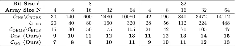
Bit Size` 8 32
Array Size N 4 8 16 32 64 4 8 16 32 64
CINS\CBUBS 30 140 600 2480 10080 42 196 840 3472 14112
COES 20 40 80 160 320 28 56 112 224 448
COEMS\CBITS 15 30 50 75 105 21 42 70 105 147
CDS (Ours) 9 10 11 12 13 11 12 13 14 15
CGS (Ours) 7 8 9 10 11 9 10 11 12 13
Table 1: The multiplicative depth of different sorting circuits given sizeN and`
Parameter Selection. According to [11] the NTRU based SWHE Scheme requires Hermite factor δ < 1.0066 to achieve a security level of 80-bit. We set the per level cutting rate logpdepending both on the circuit itself and its total depth, similarly we choose a polynomial degreenaccording to security threshold and maximum coefficient modulus size. We implementedCOES,COEMS,CDSandCGScircuits, simulated them
for both`= 8-bit and`= 32-bit integer inputs and selected array sizeN as powers of two5. In Table 2 (see
Appendix), we enumerate the parameters which we used in our experiments for various circuit depths. The largest Hermite factor among our parameter choices isδ= 1.0060, ensuring a security level of 99-bits, which is the lowest security level for all cases.
Depth d 9 12 15 21 28 42 56
logp 20 20 22 25 25 25 30
logq0 200 260 352 550 725 1075 1710
n 8190 8190 16384 16384 27000 32768 46656
S 630 630 1024 1024 1800 2048 2592
δ 1.0041 1.0054 1.0037 1.0057 1.0046 1.0056 1.0063
Table 2: Cutting size logp, maximum coefficient size logq0, Polynomial degreen, message batching slot size
S and Hermite Factorδfor different depthsd
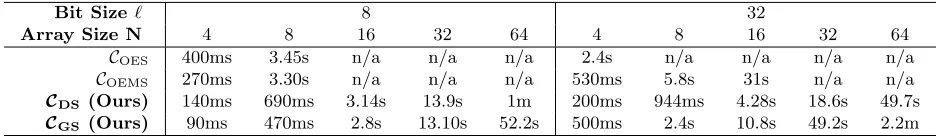
Performance Results. We implemented homomorphic Odd Even Sort, Batcher’s Odd Even Merge Sort and both of the proposed algorithms in C++ using DHS-SWHE Library [11]. All simulations were performed on an Intel Xeon @ 2.9 GHz server running Ubuntu Linux 13.10. We compiled our code using Shoup’s NTL library version 6.0 and with GMP version 5.1.3. The sorting times for 8 and 32 bit integers are given in Table 3. ForN = 64 our algorithm runs in about 14.15 hours whereas the amortized running time, where we use batching with slot size 630, is about 1.35 minutes per sort. ForN = 4 the sorting takes as low as 0.20 seconds per sort. In comparison, the homomorphic Lazy Sort implementation of [8] takes about 976 and 1400 seconds for array sizes of 10 and 40, respectively. For array sizes N = 16 and N = 64 our implementation takes 4.28 and 50 seconds, respectively.
7
Conclusion
We proposed two depth optimized sorting algorithms for efficient homomorphic evaluation. Circuit depth is intimately related to the parameter sizes in leveled homomorphic encryption implementations and therefore directly affect the overall performance of the homomorphic circuit evaluation. Existing sorting algorithms are not optimized for homomorphic evaluation. To close this gap we presented the depth analysis for several classical sorting algorithms: Bubble sort, Insertion Sort, Odd Even Sort, Odd Even Merge Sort, Merge Sort, and Bitonic Sort. Inspired by the performance of Merge Sort we introduced two new depth-optimized sorting algorithms which achieve a circuit depth ofO(log(N) + log(`)).
Bit Size` 8 32
Array Size N 4 8 16 32 64 4 8 16 32 64
COES 400ms 3.45s n/a n/a n/a 2.4s n/a n/a n/a n/a
COEMS 270ms 3.30s n/a n/a n/a 530ms 5.8s 31s n/a n/a
CDS (Ours) 140ms 690ms 3.14s 13.9s 1m 200ms 944ms 4.28s 18.6s 49.7s CGS(Ours) 90ms 470ms 2.8s 13.10s 52.2s 500ms 2.4s 10.8s 49.2s 2.2m
Table 3: Amortized execution time of circuits for different array sizesN and input bit sizes`
To study the real-life performance of our sorting algorithms, we instantiated an NTRU based SWHE scheme in the DHS SWHE library and presented simulation results for selected array lengths. For this we determined the ideal parameter choices, e.g. modulus cutting levels to cope with noise growth and Hermite work factor estimates to ensure reasonable security margins. The implementation performs favorably achieving significant speedup over the proposal in [8] for similar array lengths.
References
1. Batcher, K.E.: Sorting networks and their applications. In: Proceedings of the April 30–May 2, 1968, Spring Joint Computer Conference. pp. 307–314. AFIPS ’68 (Spring), ACM, New York, NY, USA (1968),http://doi.acm. org/10.1145/1468075.1468121
2. Bos, J.W., Lauter, K., Naehrig, M.: Private predictive analysis on encrypted medical data. Tech. Rep. MSR-TR-2013-81 (September 2013),http://research.microsoft.com/apps/pubs/default.aspx?id=200652
3. Bos, J., Lauter, K., Loftus, J., Naehrig, M.: Improved security for a ring-based fully homomorphic encryption scheme. In: Stam, M. (ed.) Cryptography and Coding, Lecture Notes in Computer Science, vol. 8308, pp. 45–64. Springer Berlin Heidelberg (2013),http://dx.doi.org/10.1007/978-3-642-45239-0_4
4. Brakerski, Z.: Fully homomorphic encryption without modulus switching from classical gapSVP. IACR Cryptol-ogy ePrint Archive 2012, 78 (2012)
5. Brakerski, Z., Gentry, C., Vaikuntanathan, V.: Fully homomorphic encryption without bootstrapping. Electronic Colloquium on Computational Complexity (ECCC) 18, 111 (2011)
6. Brakerski, Z., Vaikuntanathan, V.: Efficient fully homomorphic encryption from (standard) LWE. In: FOCS. pp. 97–106 (2011)
7. Brenner M., Perl H., S.M.: libscarab software library.,https://hcrypt.com/
8. Chatterjee, A., Kaushal, M., Sengupta, I.: Accelerating sorting of fully homomorphic encrypted data. In: Paul, G., Vaudenay, S. (eds.) Progress in Cryptology ? INDOCRYPT 2013, Lecture Notes in Computer Science, vol. 8250, pp. 262–273. Springer International Publishing (2013),http://dx.doi.org/10.1007/978-3-319-03515-4_17 9. Cheon, Jung Hee, M.K., Lauter., K.: Secure dna-sequence analysis on encrypted dna nucleotides.,http://media.
eurekalert.org/aaasnewsroom/MCM/\discretionary{-}{}{}FIL_000000001439/EncryptedSW.pdf
10. van Dijk, M., Gentry, C., Halevi, S., Vaikuntanathan, V.: Fully homomorphic encryption over the integers. In: EUROCRYPT. pp. 24–43 (2010)
11. Dor¨oz, Y., Hu, Y., Sunar, B.: Homomorphic aes evaluation using ntru (2014),https://eprint.iacr.org/2014/ 039.pdf, iACR ePrint Archive
12. Dor¨oz, Y., Sunar, B., Hammouri, G.: Bandwidth efficient pir from ntru. In: Bhme, R., Brenner, M., Moore, T., Smith, M. (eds.) Financial Cryptography and Data Security, Lecture Notes in Computer Science, vol. 8438, pp. 195–207. Springer Berlin Heidelberg (2014),http://dx.doi.org/10.1007/978-3-662-44774-1_16
13. Fischlin, M.: A cost-effective pay-per-multiplication comparison method for millionaires (2001) 14. Gentry, C.: A Fully Homomorphic Encryption Scheme. Ph.D. thesis, Stanford University (2009) 15. Gentry, C.: Fully homomorphic encryption using ideal lattices. In: STOC. pp. 169–178 (2009)
16. Gentry, C., Halevi, S.: Implementing Gentry’s fully-homomorphic encryption scheme. In: EUROCRYPT. pp. 129–148 (2011)
17. Gentry, C., Halevi, S., Smart, N.P.: Fully homomorphic encryption with polylog overhead. IACR Cryptology ePrint Archive Report 2011/566 (2011),http://eprint.iacr.org/
19. Goldwasser, S., Micali, S.: Probabilistic encryption & how to play mental poker keeping secret all partial information. In: Proceedings of the Fourteenth Annual ACM Symposium on Theory of Computing. pp. 365–377. STOC ’82, ACM, New York, NY, USA (1982),http://doi.acm.org/10.1145/800070.802212
20. Graepel, T., Lauter, K., Naehrig, M.: Ml confidential: Machine learning on encrypted data. In: Kwon, T., Lee, M.K., Kwon, D. (eds.) Information Security and Cryptology ? ICISC 2012, Lecture Notes in Computer Science, vol. 7839, pp. 1–21. Springer Berlin Heidelberg (2013),http://dx.doi.org/10.1007/978-3-642-37682-5_1 21. Knuth, D.E.: The Art of Computer Programming, Fundamental Algorithms, vol. 1. Addison Wesley Longman
Publishing Co., Inc., 3rd edn. (1998), (book)
22. Lagendijk, R., Erkin, Z., Barni, M.: Encrypted signal processing for privacy protection: Conveying the utility of homomorphic encryption and multiparty computation. Signal Processing Magazine, IEEE 30(1), 82–105 (Jan 2013)
23. Lauter, K., Naehrig, M., Vaikuntanathan, V.: Can homomorphic encryption be practical. Cloud Computing Security Workshop pp. 113–124 (2011)
24. Lauter, K., Lopez-Alt, A., Naehrig, M.: Private computation on encrypted genomic data. Tech. Rep. MSR-TR-2014-93 (June 2014),http://research.microsoft.com/apps/pubs/default.aspx?id=219979
25. L´opez-Alt, A., Tromer, E., Vaikuntanathan, V.: On-the-fly multiparty computation on the cloud via multikey fully homomorphic encryption. In: STOC (2012)
26. L´opez-Alt, A., Naehrig., M.: Large integer plaintexts in ring-based fully homomorphic encryption. in preparation (2014)
27. Rivest, R.L., Adleman, L., Dertouzos, M.L.: On data banks and privacy homomorphisms. Foundations of Secure Computation pp. 169–180 (1978)
28. Sander, T., Young, A., Yung, M.: Non-interactive cryptocomputing for nc1. In: Foundations of Computer Science, 1999. 40th Annual Symposium on. pp. 554–566 (1999)
29. Smart, N.P., Vercauteren, F.: Fully homomorphic SIMD operations. IACR Cryptology ePrint Archive 2011, 133 (2011)
30. Stehl´e, D., Steinfeld, R.: Making ntru as secure as worst-case problems over ideal lattices. Advances in Cryptology – EUROCRYPT ’11 pp. 27–4 (2011)
31. Vaidya, J., Clifton, C.: Privacy-preserving k-means clustering over vertically partitioned data. In: Proceedings of the Ninth ACM SIGKDD International Conference on Knowledge Discovery and Data Mining. pp. 206–215. KDD ’03, ACM, New York, NY, USA (2003),http://doi.acm.org/10.1145/956750.956776
32. Yao, A.C.: Protocols for secure computations. In: Proceedings of the 23rd Annual Symposium on Foundations of Computer Science. pp. 160–164. SFCS ’82, IEEE Computer Society, Washington, DC, USA (1982), http: //dx.doi.org/10.1109/SFCS.1982.88