DEL ROSARIO, RICARDO CRUZ-HERRERA. Computational Methods for Feed-back Control in Structural Systems. (Under the direction of Prof. H.T. Banks)
CONTROL IN STRUCTURAL SYSTEMS
by
RICARDO C.H. DEL ROSARIO
a dissertation submitted to the graduate faculty of
north carolina state university
in partial fulfillment of the
requirements for the degree of
doctor of philosophy
department of mathematics
raleigh
August 26, 1998
Ricardo Cruz-Herrera del Rosario was born in Olongapo City, Philippines on January 26, 1970, where he spent the first 12 years of his life. In June 1982, he moved to Manila to study at Philippine Science High School in Diliman, Quezon City. He later attended the University of the Philippines in Diliman from June 1986 to October 1989 where he graduated Cum Laude with a Bachelor of Science in Mathematics. For the next two years he worked as an instructor in the Department of Mathematics at the University of the Philippines while taking graduate courses in actuarial and computer science. Tokyo Denshi Sekkei Philippines, Inc. then hired him as a software engineer from November 1991 to July 1993. In August 1993, he moved to the United States to continue his graduate studies. He obtained his M.S. degree in Mathematics from Iowa State University in May 1995 and afterwards spent two months as a summer intern at NASA Langley Research Center. He started his doctoral studies in Applied Mathematics at North Carolina State University in August 1995.
A lot of people made it possible for me to finish this dissertation. For guidance and support through my graduate studies at NC State, I thank my advisor Prof. H. T. Banks. For continued advice and friendship since I was a masters student at Iowa State University, I am grateful to Prof. Ralph Smith. I also express sincere appreciation to Professors Hien Tran and Kazufumi Ito for valuable input on various aspects of my research.
I gratefully acknowledge the Air Force Office of Scientific Research for financial support under grants AFSOR F49620-95-1-0236 and AFSOR F49620-98-1-0180. Ad-ditional support was also provided in part by the National Aeronautics and Space Administration under NASA Contract Number NAS1-19480 and NASA grant NAG-1-1600.
I extend deepest gratitude to all my friends who encouraged and helped me throughout the process. Special thanks to Melissa Choi, Laura Potter, Cindy Mu-sante, Mike Jeffris, Yue Zhang, Rebecca Segal, John Peach, Rory Schnell, Hung Ly, Gerald Guanga, Karyna Ventura, Jennifer Pizarro and Myrene Santos.
I am indebted to Jose and Tessie Chua, Lorrie and Wyda Chua, Francis and Sony Jao, and Ricky and Arlete Chua for making me a part of their family.
Finally, I would like to thank my parents Cecinio and Lourdes, my brother Dante and his wife Peeya, and my sisters Belinda, Laura and Melissa for their unconditional love and support.
List of Tables vii
List of Figures ix
List of Symbols x
1 Introduction 1
2 Shell Equations 5
3 Abstract Formulation and Feedback Control 14
3.1 Variational Formulation . . . 14
3.2 Semigroup Formulation . . . 18
3.3 Control Problem . . . 20
3.4 Convergence of Finite Dimensional Approximations . . . 23
3.5 Finite Dimensional Control and Convergence of Riccati Solutions . . 25
4 Approximation Methods 36 4.1 Full Order Methods . . . 42
4.2 Lagrange Reduced Basis Method . . . 47
4.3 POD Reduced Basis Method . . . 48
5 Numerical Examples 52 5.1 Full Order Methods . . . 55
5.1.1 Modal Solutions . . . 55
5.1.2 Uncontrolled Simulations . . . 74
5.1.3 LQR Control . . . 96
5.2 Reduced Basis Methods . . . 111
5.2.1 Uncontrolled Simulations . . . 112
5.2.2 LQR Control . . . 116
6 Conclusions 125
List of References 127
A Passive Patch Contributions 133
B V inner product definition 136
C Weak Form and Matrix Components 139
C.1 Circumferential Displacement . . . 139 C.2 Transverse Displacement . . . 142
4.1 Basis functions for simply-supported models . . . 46
4.2 Basis functions for clamped-edge models . . . 46
5.1 English system shell and patch parameters . . . 53
5.2 Metric system shell and patch parameters . . . 53
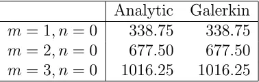
5.3 Simply supported frequencies withm= 0 . . . 61
5.4 Simply supported frequencies withm= 0 using linear splines . . . 64
5.5 Simply supported frequencies withn= 0 . . . 64
5.6 General simply supported frequencies . . . 67
5.7 Accuracy of cubic spline frequency approximation . . . 68
5.8 Fixed-edge cubic spline frequencies withM = 0 and N = 16 . . . 74
5.9 Discretization sizes for mixed linear/cubic splines . . . 78
5.10 Absolute errors using mixed linear/cubic splines, steady state . . . . 79
5.11 O‘ (h2 x) convergence with mixed linear/cubic splines, steady state . . . 80
5.12 Discretization sizes for cubic splines . . . 82
5.13 Absolute errors using cubic splines, steady state . . . 83
5.14 O‘ (h4 x) convergence with cubic splines, steady state. . . 84
5.15 Stiffness ratios for the system matrix A2N . . . . 86
5.16 Absolute errors using cubic splines, time dependent . . . 87
5.17 O‘ (h4 x) convergence with cubic splines, time dependent, T = 1.5sec. . 88
5.18 Approximate natural frequencies of the damped shell . . . 92
5.19 Approximate natural frequencies of the lightly damped shell . . . 94
5.20 Passive patch contribution effects on frequencies . . . 95
5.21 `1 norm of difference between full and Lagrange reduced models . . . 113
5.22 Percent of “energy” captured by POD reduced basis method . . . 114
5.23 `1 norm of difference between full and POD reduced models . . . 114
5.24 Ranks of the controllability matrix C(A2NP, B2NP) . . . . 122
2.1 Thin cylindrical shell with piezoceramic patch configuration. . . 8
2.2 In-phase patch excitation . . . 11
2.3 Out-of-phase patch excitation . . . 12
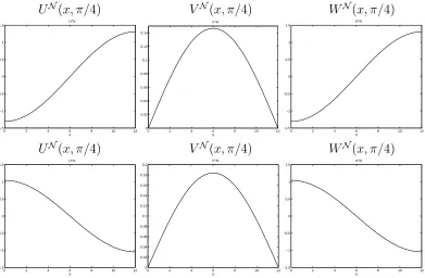
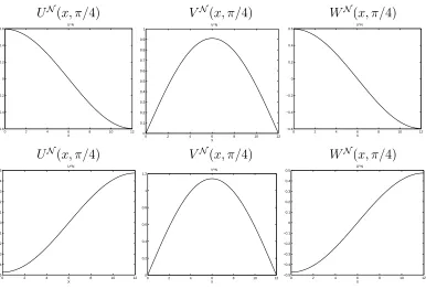
5.1 Simply supported axisymmetric modes (m= 0, n= 1) . . . 62
5.2 Simply supported axisymmetric modes (m= 0, n= 2) . . . 63
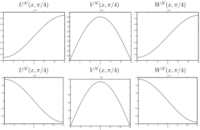
5.3 Purely extensional modes in the longitudinal direction . . . 65
5.4 Components of the 147.09 Hz modes . . . 66
5.5 Components of the 508.59 Hz modes . . . 68
5.6 Components of the 1873.61 Hz modes . . . 69
5.7 Fixed-edge axisymmetric torsional modes . . . 71
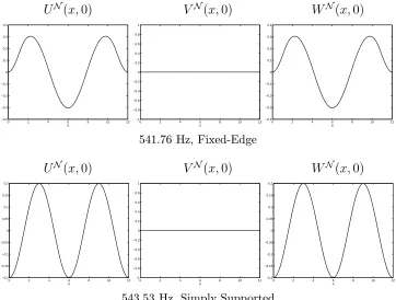
5.8 Fixed-edge and simply supported modes around 542 Hz . . . 72
5.9 Fixed-edge and simply supported modes around 545 Hz . . . 73
5.10 True solutions for steady state example . . . 77
5.11 Approximate uN using mixed linear/cubic splines, steady state . . . . 79
5.12 Approximate vN using mixed linear/cubic splines, steady state . . . . 80
5.13 Approximate wN using mixed linear/cubic splines, steady state . . . 81
5.14 Steady state errors using cubic splines . . . 83
5.15 True solutions for time dependent example . . . 87
5.16 Time dependent errors using cubic splines . . . 88
5.17 Temporal voltage applied to the patch. . . 90
5.18 Displacements and frequencies in u of the damped shell . . . 90
5.19 Displacements and frequencies in v of the damped shell . . . 91
5.20 Displacements and frequencies in w of the damped shell . . . 91
5.21 Displacements and frequencies in u of the lightly damped shell . . . . 93
5.22 Displacements and frequencies in v of the lightly damped shell . . . . 93
5.23 Displacements and frequencies in w of the lightly damped shell . . . . 94
5.24 Location of p1,L1 and L2 on the shell, and normal external force . . 97
5.25 Full order time histories (g = 0) . . . 100
5.26 Full order rms plots (g = 0) . . . 101
5.28 Full order rms plots (single frequency, small patch) . . . 104
5.29 Full order time histories (single frequency, large patch) . . . 105
5.30 Full order rms plots (single frequency, large patch) . . . 106
5.31 Full order time histories (multiple frequency, small patch) . . . 108
5.32 Full order rms plots (multiple frequency, small patch) . . . 109
5.33 Voltages to control multiple frequency excitation . . . 110
5.34 Sum of inner and outer voltages to patch pair 1. . . 111
5.35 Uncontrolled time histories at p1 of the reduced order methods . . . . 115
5.36 Reduced basis rms displacements . . . 116
5.37 Controlled time histories at p1 of the reduced basis methods . . . 117
5.38 Time histories; control design based on N = 9 POD functions . . . . 123
5.39 Rms displacements; control design based on N = 9 POD functions . . 124
u longitudinal displacement
v circumferential displacement
w transverse displacement
R shell radius
E shell Young’s Modulus
` shell length
ρ shell density
h shell thickness
cD shell Kelvin-Voigt damping
ν shell Poisson ratio
d31 patch proportionality constant 1i, pe1i subscripts to identifyith outer patch
2i, pe2i subscripts to identifyith inner patch
ˆ
qx surface force in longitudinal direction
ˆ
qθ surface force in circumferential direction
ˆ
qn surface force in transverse direction
V, V test function spaces; V =V ×V H, H state spaces; H=H×V
U control space (lR2s)
Y observation space
Nu, Nv, Nw no. of standard splines in u, v, wdirections
Mu, Mv, Mw no. of Fourier limits in circumferential direction
M indicates the same no. of Fourier limits M =Mu =Mv =Mw
Nu,Nv,Nw no. of basis functions in u, v, w directions
N dimension of subspaceVN ⊂V (N =Nu+Nv+Nw)
2N dimension of subspaceV2N =VN ×VN ⊂ V
A,A2N infinite and finite dimensional system operators
B,B2N infinite and finite dimensional control operators
C,C2N infinite and finite dimensional observation operators
A2N matrix representation of A2N
B2N matrix representation of B2N
Introduction
Advances in smart material technologies have produced a number of lightweight ma-terials whose sensing and actuating capabilities are promising in control applications (for a general discussion on current smart materials used in smart material struc-tures, see [14]). Control methodologies have kept pace by considering the physical properties of the structure/sensor system thereby establishing control authority with less hardware and control input. Recent demands in smart material control applica-tions include faster methods to compute feedback control gains. We aim to address this by presenting a numerical approximation method which (i) captures the essential dynamics of the system to be controlled, (ii) is easily adaptable to different bound-ary conditions, (iii) allows material changes when smart materials are incorporated into the system, and (iv) concentrates most numerical computations off-line for faster control gain calculations. We focus on a system consisting of a thin cylindrical shell bonded with piezoceramic patches as actuators but the numerical methods and con-trol methodologies we present are readily implementable for other structures such as plates or beams, employing different types of smart actuators such as electrostrictives or magnetostrictives.
Piezoceramic patches, as actuators, produce strains in response to applied volt-ages; as sensors, material deformations of the structure to which they are bonded or in which they are embedded generate voltages. These smart materials are preferred for
control applications in thin shell dynamics since they are lightweight, cost effective, easily manufactured in different sizes and shapes, produce significant strains, and the voltage-strain relations are nearly linear for small electric fields. It must be noted that at higher fields, nonlinear responses occur which can degrade the control design if the nonlinearities are not part of the design. For current applications, the voltage limits are within the linear range of the piezoceramic patch. High temperatures can change the constant relation between generated strain and patch input. Hence for systems subjected to above normal temperatures, parameter identification must be performed (see [14]) once the constant has changed.
Active control of shell vibrations has been a growing research area for a number of years due to its vast number of applications such as noise and fatigue reduction in aircraft cabins, vibration suppression for the cylindrical support coils in magnetic resonance image equipments, and flow control in flexible pipes. Mathematical models of thin shells, accepted as the primary tool in this field, abound in literature. The existing models differ on assumptions made to express the strain-displacement equa-tions of linear elasticity. In [34, 38], a summary and comparison of the theories of Donnell-Mushtari, Love-Timoshenko, Byrne-Fl¨ugge-Goldenveizer-Lur’ye-Novozhilov, Reissner-Naghdi-Berry and Vlasov and Sanders are given. The model of Koiter is one of the latest improvements to the Love-Kirchhoff family of thin shell models (see [17]). We chose to express shell dynamics through the Donnell-Mushtari equations because this framework, aside from providing ease in exposition while capturing the essential dynamics of relatively short shells (i.e., the ratio of the length ` over the radius R is less than 1/4), has the advantage of being easily extended to more accurate models (Naghdi or Sanders) or longer shells (Fl¨ugge).
easily adaptable to different boundary conditions and a number of books and soft-ware packages have been written for thin shell approximation (see [4, 17, 27, 26, 28, 53]). Discontinuities in shell constants and parameters which arise when piezoceramic patches are bonded to the shell pose difficulties in the creation of the elements. In such cases, the elements must be aligned with the boundaries of the patches. An-other difficulty with finite element methods is the locking phenomena which can be exhibited when elements are not able to handle the Kirchhoff-Love constraint of van-ishing transverse shear strains as the shell thickness htends to zero ([3, 15]). Another more serious type of locking arises when the approximation method is not capable of handling purely bending deformation energies (see [5, 6, 33, 45]). In this case, mesh sizes must be decreased significantly smaller than the shell thickness to accommodate higher order finite elements in bending dominated simulations. Modal approximation methods are useful only in applications where analytic expressions for the modes can be obtained. For most applications, however, mode shapes must be first approximated or experimentally determined before being used in the modal expansions.
We present a Galerkin type approximation method employing spline bases in the axial direction and Fourier polynomials in the circumferential (θ) direction. Although we show in Chapter 5 that several of the issues in numerical approximation are suc-cessfully resolved with this method, a need still exists for faster calculations. Hence we investigate the Lagrange and Karhunen-Lo`eve proper orthogonal decomposition (POD) reduced basis methods in an attempt to decrease the size of the finite dimen-sional system. The first attempts at reduced basis methods in structures appear to have been by Almroth [2] and Nagy [39]. Preliminary applications in structures can also be found in [40, 41, 42], while implementation in incompressible viscous flows were pioneered by Peterson [44]. In open loop control of fluids, we believe that the Lagrange reduced basis method was first employed in [30, 31] and POD was first used in [37]. To our knowledge, this thesis (and [7]) represent the first time Lagrange or POD reduced basis functions are employed infeedback control of structures.
functions, where the “solutions” could come either from numerical simulations or experimental data. The idea is based on the hope that solutions at other parameter values could be approximated in terms of the few chosen representative parameters. Proper orthogonal reduced basis methods initially use the same parameter dependent “solutions” but an optimal way of capturing the features in the “solutions” is obtained through an orthogonalization procedure. Out of the initial set of parameter dependent solutions, a smaller set of orthogonal solutions containing most of the information in the first set, are used as basis functions.
Shell Equations
The system we consider in this dissertation is a thin cylindrical shell with surface-mounted piezoceramic patches as actuators. In accordance with thin shell theory, the shell is assumed to satisfy four basic assumptions, known as Love’s postulates, namely (i) the thickness h of the shell is small compared to the radius R, i.e., h/R 1; (ii) shell deflections are assumed to be small; (iii) the stress in the direction normal to the thin dimensions is assumed negligible, and (iv) a line originally normal to the shell reference surface will remain normal to the deformed reference surface, and unstrained (see [14, 34, 35]). Shell dynamics are modeled using the Donnell-Mushtari equations and hence it is assumed that the ratio of the length ` of the shell to its radius is less than 4. Furthermore, it is assumed that the shell thickness is uniform. Bonded to the inner and outer surfaces of the shell are s pairs of piezoceramic patches which will be used as actuators in this work. The actuating capabilities of the patches derive from material deformations which occur in response to applied voltages. The patches also produce voltages in response to mechanical strains but the sensing capacity is not exploited here. Piezoceramic patches can be molded in a variety of shapes and so, as in many applications, we assume that the patches are molded to have the same curvature as the shell. This does not cause pre-stressing on the structure but significantly alters the material properties as well as the thickness of the structure in regions covered by the patches. These passive patch contributions enter the equations by changing the
internal moments and forces of the shell. Contributions to the structural dynamics due to the glue bonding layer are ignored. It is demonstrated in [14] that these contributions can be combined with passive patch contributions, and the resulting coefficients can be obtained using parameter estimation techniques.
According to assumption (ii) above, shell deflections are small hence all displace-ments are measured from the original, undeformed state of the shell. The fourth as-sumption (iv) assumes that displacements in the thickness direction are linear hence every point on the shell surface can be described by the corresponding point on the reference surface. We choose the unperturbed middle surface of the shell to be the reference surface. All forces and moments are thus given in terms of middle surface resultants.
As illustrated in Figure 2.1, we orient the shell such that its longitudinal axis is aligned with the x-axis. The displacements of the middle surface in the longi-tudinal, circumferential and transverse directions are denoted by u, v and w, re-spectively. The region occupied by the middle surface is denoted by Γ0 where Γ0 = {(x, θ) : 0≤x≤`,0≤θ≤2π}; the density, Young’s modulus, Poisson ratio and Kelvin-Voigt damping coefficient of the shell are denoted by ρs, E, ν and cD,
respectively. Also indicated in Figure 2.1 is the location of the ith outer patch
with center located at (¯x1i,θ¯1i) and edge coordinates x11i, x21i, θ11i, θ11i. The
cen-ter of the ith inner patch will be denoted similarly by (¯x2i,θ¯2i) with edge coordinates
x12i, x22i, θ12i, θ12i. For the rest of this paper, the subscripts 1i and 2i will be used
to identify the ith outer and inner patches, respectively. It is assumed that for the
ith patch pair, the outer patch has thickness h
pe1i, density ρpe1i, Young’s modulus Epe1i, Poisson ratio νpe1i, Kelvin-Voigt damping coefficient cDpe1i and proportionality
constant d311i. Similarly, the inner patch properties will be denoted by hpe2i, ρpe2i, Epe2i, νpe2i, cDpe2i and d31. The proportionality constant d311i (see [14, 29]) relates
the design of the smart material system, and to account for inconsistencies in cur-rent manufacturing methods for piezoceramic patches. Furthermore, the model and control formulation permit different voltage inputs to the 2s patches.
Shell equations are derived in [14, 34] by considering strain-displacement rela-tions, stress-strain relarela-tions, internal force and moment resultants, and equations of motion. By neglecting higher order terms, one obtains the modified Donnell-Mushtari equations
Rρh∂
2u
∂t2 −R
∂Nx
∂x −
∂Nθx
∂θ =Rqˆx
−R
s X
i=1
"
∂(Nx)pe1i
∂x Spe1i(x, θ) +
∂(Nx)pe2i
∂x Spe2i(x, θ)
#
Rρh∂
2v
∂t2 −
∂Nθ
∂θ −R
Nxθ
∂x =Rqˆθ
−Xs
i=1
"
∂(Nθ)pe1i
∂θ Spe1i(x, θ) +
∂(Nθ)pe2i
∂θ Spe2i(x, θ)
#
Rρh∂
2w
∂t2 −R
∂2M
x
∂x2 −
1
R
∂2M
θ
∂θ2 −2
∂2M
xθ
∂x∂θ +Nθ =Rqˆn
−Xs
i=1
"
R ∂
2
∂x2
(Mx)pe1i + (Mx)pe2i
+ 1
R
∂2
∂θ2
(Mθ)pe1i+ (Mθ)pe2i
#
.
(2.1)
External resultant forces in the longitudinal, circumferential and transverse directions are modeled by the functions ˆqx,qˆθ and ˆqn, respectively (see [14]).
The composite densityρconsists of the shell densityρsin regions devoid of patches
and a linear combination of ρs and the patch densities ρpe1i, ρpe2i in regions covered
by the patches. Henceρis piecewise constant with discontinuities at the patch edges.
Figure 2.1: Thin cylindrical shell with piezoceramic patch configuration.
Nx, Nθ, Nxθ, Nθx, Mx, Mθ, Mxθ incorporating Kelvin-Voigt damping but without
pas-sive patch contributions have the form
Nx =
Eh
(1−ν2)
"
∂u
∂x +ν
1 R ∂v ∂θ + w R !#
+ cDh (1−ν2)
∂ ∂t
"
∂u
∂x +ν
1 R ∂v ∂θ + w R !#
Nθ =
Eh
(1−ν2)
" 1 R ∂v ∂θ + w
R +ν
∂u ∂x
#
+ cDh (1−ν2)
∂ ∂t " 1 R ∂v ∂θ + w
R +ν
∂u ∂x
#
Nxθ =Nθx =
Eh
2(1 +ν)
" ∂v ∂x + 1 R ∂u ∂θ #
+ cDh 2(1 +ν)
∂ ∂t " ∂v ∂x + 1 R ∂u ∂θ #
Mx =−
Eh3
12(1−ν2)
"
∂2w
∂x2 +
ν
R2
∂2w
∂θ2
#
− cDh3
12(1−ν2)
∂ ∂t
"
∂2w
∂x2 +
ν
R2
∂2w
∂θ2
#
Mθ =−
Eh3
12(1−ν2)
"
1
R2
∂2w
∂θ2 +ν
∂2w
∂x2
#
− cDh3
12(1−ν2)
∂ ∂t
"
1
R2
∂2w
∂θ2 +ν
∂2w
∂x2
#
Mxθ =Mθx =−
Eh3
12R(1 +ν)
∂2w
∂x∂θ −
cDh3
12R(1 +ν)
∂ ∂t
"
∂2w
∂x∂θ
#
.
We point out that these resultants yield the classical Donnell-Mushtari equations if the damping terms are dropped, i.e., set cD = 0 (see [34]). Incorporation of passive
patch contributions in the model leads to the addition of more terms in the resultant expressions. In this case, the internal force Nx is now given by
Nx =
Eh
(1−ν2)
"
∂u
∂x +ν
1 R ∂v ∂θ + w R !# + s X i=1
Epe1i
(1−ν2
pe1i)
"
hpe1i ∂u
∂x +νpe1i
1 R ∂v ∂θ + w R !!
−a21i
2
∂2w
∂x2 +
νpe1i
R2
∂2w
∂θ2
!#
χpe1i(x, θ)
+
s X
i=1
Epe2i
(1−ν2
pe2i)
"
hpe2i ∂u
∂x +νpe2i
1 R ∂v ∂θ + w R !! (2.3)
+a22i
2
∂2w
∂x2 +
νpe2i
R2
∂2w
∂θ2
!#
χpe2i(x, θ)
+ cDh (1−ν2)
∂ ∂t
"
∂u
∂x +ν
1 R ∂v ∂θ + w R !# + s X i=1
cDpe1i
(1−ν2
pe1i) ∂ ∂t
"
hpe1i ∂u
∂x +νpe1i
1 R ∂v ∂θ + w R !!
−a21i
2
∂2w
∂x2 +
νpe1i
R2
∂2w
∂θ2
!#
χpe1i(x, θ)
+
s X
i=1
cDpe2i
(1−ν2
pe2i) ∂ ∂t
"
hpe2i ∂u
∂x +νpe2i
1 R ∂v ∂θ + w R !!
+a22i
2
∂2w
∂x2 +
νpe2i
R2
∂2w
∂θ2
!#
χpe2i(x, θ) .
Expressions for Nθ, Nxθ, Nθx, Mx, Mθ and Mxθ with passive patch contributions are
in the expressions above, the presence of the characteristic function χpe1i(x, θ) with
value 1 in the region covered by the ith outer patch and zero elsewhere indicates
the patch contributions to regions of the shell covered by the patch, with χpe2i(x, θ)
defined analogously. Furthermore, the constants a21i = (h/2 +hpe1i)
2−h2/4, a 22i =
(h/2 +hpe2i)
2−h2/4, a
31i = (h/2 +hpe1i)
3 −h3/8 and a
32i = (h/2 +hpe2i)
3 −h3/8 arise from integrating across the thickness of the patch.
Denoting the outer and inner input voltages by V1i(t) andV2i(t), respectively, the
external line force and moment resultants due to theith patch pair, as derived in [14],
are given by
(Mx)pe1i =
−Epe1id311i
(1−νpe1i)hpe1i
1
2a21i +
1 3Ra31i
χpe1i(x, θ)V1i
(Mx)pe2i =
Epe2id312i
(1−νpe2i)hpe2i
1
2a22i −
1 3Ra32i
χpe2i(x, θ)V2i
(Mθ)pe1i = −
Epe1id311ia21i
2(1−νpe1i)hpe1i
χpe1i(x, θ)V1i
(Mθ)pe2i =
Epe2id312ia22i
2(1−νpe2i)hpe2i
χpe2i(x, θ)V2i (2.4)
(Nx)pe1i = −
Epe1id311i
(1−νpe1i)hpe1i
hpe1i+
1 2a21i
χpe1i(x, θ)Spe1i(x, θ)V1i
(Nx)pe2i =
−Epe2id312i
(1−νpe2i)hpe2i
hpe2i−
1 2a22i
χpe2i(x, θ)Spe2i(x, θ)V2i
(Nθ)pe1i =
−Epe1id311i
1−νpe1i
χpe1i(x, θ)Spe1i(x, θ)V1i
(Nθ)pe2i =
−Epe2id312i
1−νpe2i
χpe2i(x, θ)Spe2i(x, θ)V2i
The patch-induced external resultants (Nx)pe1i and (Nθ)pe1i produce forces which are
opposite in direction at points symmetric to the center (¯x1i,θ¯1i) of the ith outer
Figure 2.2: In-phase patch excitation producing predominantly planar vibrations.
Spe1i(x) ˆSpe1i(θ), where
Spe1i(x) =
1 , x <(x11i+x21i)/2
0 , x= (x11i+x21i)/2
−1 , x >(x11i+x21i)/2
,
and
ˆ
Spe1i(θ) =
1 , θ <(θ11i+θ21i)/2
0 , θ= (θ11i+θ21i)/2
−1 , θ >(θ11i+θ21i)/2
.
The indicator function Spe2i(x, θ) =Spe2i(x) ˆSpe2i(θ) for the inner patches is similarly
defined by replacing the subscripts i1 with 2i in the definitions above.
If predominantly planar vibrations are needed, we model identical voltages applied to the ith patch pair as indicated in Figure 2.2. To obtain predominantly bending
deformations, we model voltages with the same magnitude but opposite signs, as depicted in Figure 2.3. As indicated later in Chapter 5, the control methods we employ to stabilize an externally excited shell necessitate voltage inputs to the inner and outer patches which are nearly diametrically out-of-phase but exhibit magnitude differences. This indicates that both in-plane forces and bending moments are generated.
Figure 2.3: Out-of-phase patch excitation producing predominantly bending mo-ments.
clamped edge and simply supported boundary conditions. The clamped edge condi-tions are expressed as
u(t,0, θ) =u(t, `, θ) = v(t,0, θ) =v(t, `, θ) = 0 (2.5a)
w(t,0, θ) =w(t, `, θ) = ∂w(t,0, θ)
∂x =
∂w(t, `, θ)
∂x = 0 , (2.5b)
(see [14]), while simply supported boundary conditions are given by
v(t,0, θ) =v(t, `, θ) = w(t,0, θ) =w(t, `, θ) = 0 (2.6a)
Mx(t,0, θ) =Mx(t, `, θ) =Nx(t,0, θ) =Nx(t, `, θ) = 0 (2.6b)
(see [34]).
For approximation and theoretical analysis (see [24, 25]) we consider the weak form of the equations
Z
Γ0
R
(
ρh∂
2u
∂t2η1+Nx
∂η1
∂x +
1
RNθx
∂η1
∂θ −qˆxη1−
s X
i=1
(Nx)pe1i+ (Nx)pe2i
∂η
1
∂x
)
dγ= 0
Z
Γ0
(
Rρh∂
2v
∂t2η2+Nθ
∂η2
∂θ +RNxθ
∂η2
∂x −Rqˆθη2−
s X
i=1
(Nθ)pe1i+ (Nθ)pe2i
∂η
2
∂θ
)
dγ= 0
Z
Γ0
(
Rρh∂
2w
∂t2 η3+Nθη3−Rqˆnη3 −RMx
∂2η 3
∂x2 −
1
RMθ
∂2η 3
∂θ2 −2Mxθ
∂2η 3
∂x∂θ
+R
s X
i=1
(Mx)pe1i+ (Mx)pe2i
∂2η
3
∂x2 +
1
R
s X
i=1
(Mθ)pe1i+ (Mθ)pe2i
∂2η
3
∂θ2
)
dγ= 0
for all test functions Ψ = (η1, η2, η3) (see [14] for details in derivation). Here, the state variables for the system are taken to be y= (u, v, w) in the state space
H =L2(Γ0)×L2(Γ0)×L2(Γ0). (2.8)
Test functions are chosen to satisfy essential boundary conditions and smoothness criteria. For the fixed edge or clamped boundary conditions (2.5), we take the space of test and trial functions to be
V =H01(Γ0)×H01(Γ0)×H02(Γ0), (2.9)
where
H01(Γ0) =
n
η∈H1(Γ0) :η(0,·) = η(`,·) = 0
o
H02(Γ0) =
(
η∈H2(Γ0) :η(0,·) =
∂η(0,·)
∂x =η(`,·) =
∂η(`,·)
∂x = 0
)
.
On the other hand, the test and trial function space for the simply supported bound-ary conditions (2.6) is
V =H1(Γ0)×H01(Γ0)×H2(Γ0)∩H01(Γ0) . (2.10)
Abstract Formulation and Feedback
Control
In this section, we show well-posedness of the shell model using variational and semi-group formulations. The abstract variational form is useful in parameter estimation and numerical approximation methods, while the semigroup formulations are suit-able for control applications. We illustrate well-posedness by invoking existence and uniqueness theorems given in [14, Chapter 4]. The equivalence of the variational and semigroup solutions is also verified. We then briefly state control results on the infinite dimensional system and discuss convergence of Galerkin approximations. Existence, uniqueness and convergence of the Riccati solutions and the approximate LQR controls are illustrated following the ideas in [11, 14].
3.1
Variational Formulation
As indicated in [11, 14], we start the abstract formulation by considering Hilbert spaces V and H such that V is continuously and densely embedded in H. We then identify H∗ with H through the Riesz map, and consider the Gelfand triple V ,→ H ,→ V∗ (see [14, p. 97], [52, p. 25] or [54, p. 261]). Here V∗ and H∗ are the dual spaces to V and H, respectively. We take the duality product h·,·iV∗×V on
defined on H×V.
It can be readily shown that the test function spaceV (given in (2.9) or (2.10)) and state space H (given in (2.8)) satisfy the continuous and dense embedding conditions above, hence for the shell system, we let V ≡ V, H ≡ H with V ,→ H ,→ V∗. Furthermore, the embedding of V into H and H∗ into V∗ are compact (for details regarding the embedding of V in H, see for example, [1, 54]).
We now define the inner products on H and V to abstractly formulate the mass, stiffness and damping terms in (2.7). To this end, we define the inner product on H
to be
hφ, ψiH =
Z
Γ0
ρhuη¯1dγ+
Z
Γ0
ρhvη¯2dγ+
Z
Γ0
ρhwη¯3dγ , (3.1) whereφ= (u, v, w), ψ= (η1, η2, η3)∈H anddγ =Rdθdx. It can be readily seen that the norm induced by this inner product is equivalent to the usual norm in H. We next define the stiffness inner product h·,·iV
E on V to be
hφ, ψiV
E =
16
X
i=1
Ii(φ, ψ) , (3.2)
where the Ii are terms in the weak form containing the stiffness coefficients E, Epe1i
and Epe2i, obtained by the substitution of the internal force and moments resultants
(i.e., (2.3), (A.1), (A.2), (A.3),(A.4) and (A.5) substituted in the weak form (2.7)). To illustrate, I1 and I2 have the form
I1(φ, ψ) =
Z 2π
0
Z `
0
EhR
(1−ν2)
"
∂u
∂x +ν
1 R ∂v ∂θ + w R !# ∂η1
∂xdxdθ (3.3)
I2(φ, ψ) =
s X
i=1
Z θ21i
θ11i Z x21i
x11i
Epe1iR
(1−ν2
pe1i)
"
hpe1i ∂u
∂x +νpe1i
1 R ∂v ∂θ + w R !!
− a21i
2
∂2w
∂x2 +
νpe1i
R2
∂2w
∂θ2 !# ∂η1 ∂xdxdθ + s X i=1
Z θ22i
θ12i Z x22i
x12i
Epe2iR
(1−ν2
pe2i)
"
hpe2i ∂u
∂x +νpe2i
1 R ∂v ∂θ + w R !!
+ a22i
2
∂2w
∂x2 +
νpe2i
R2
∂2w
∂θ2
!#
∂η1
Expressions forIi, i= 4, . . . ,16 are given in Appendix B. The damping inner product
on V, denoted by < ·,· >VcD, is obtained by replacing E by cD, Epe1i by cDpe1i and Epe2ibycDpe2i in the expression for the stiffness inner producth·,·iVE given in (3.2). As
in theHinner product, the norms on V induced byh·,·iV
E andh·,·iVcD are equivalent
to the standard norm in V.
We now define the stiffness and damping sesquilinear forms σ1 :V ×V →Cl and
σ2 :V ×V →Cl , respectively, by
σ1(φ, ψ) = hφ, ψiVE
σ2(φ, ψ) = hφ, ψiV
cD +
Z
Γ0
µwη¯3dγ .
(3.5)
It is readily verified that the stiffness form σ1 satisfies
(H1) |σ1(φ, ψ)| ≤c1|φ|V |ψ|V, for some c1 ∈lR (Bounded) (H2) Reσ1(φ, φ)≥c2|φ|2V, for some c2 >0 (V-Elliptic)
(H3) σ1(φ, ψ) =σ1(ψ , φ) (Symmetric)
for all φ, ψ ∈V. Furthermore, the damping termσ2 has the properties (H4) |σ2(φ, ψ)| ≤c3|φ|V |ψ|V, for some c3 ∈lR (Bounded) (H5) Reσ2(φ, φ)≥c4|φ|
2
V, for some c4 >0 (V-Elliptic) .
From the continuity properties (H1) and (H4), it follows that we can define operators
A1,A2 ∈ L(V, V∗) such that
hA1φ, ψiV∗,V = σ1(φ, ψ), ∀φ, ψ ∈V
hA2φ, ψiV∗,V = σ2(φ, ψ), ∀φ, ψ ∈V .
(3.6)
operator ˜B ∈ L(U, V∗) is defined by
D
˜
BU(t), ψE
V∗,V = s X
i=1
Z
Γ0
[(Nx)pe1i + (Nx)pe2i]
∂η1
∂xdγ
+
s X
i=1
Z
Γ0
1
R[(Nθ)pe1i+ (Nθ)pe2i]
∂η2
∂θ dγ
− Xs
i=1
Z
Γ0
[(Mx)pe1i + (Mx)pe2i]
∂2η
3
∂x2 dγ
− Xs
i=1
Z
Γ0
1
R2 [(Mθ)pe1i+ (Mθ)pe2i]
∂2η
3
∂θ2 dγ ,
(3.7)
for all ψ = (η1, η2, η3) ∈ V and U(t) ∈ U. Note that the vector U(t) represents the time varying voltage input to each patch employed in (2.4), i.e.,
U(t) = (V11(t), V21(t), . . . , V1i(t), V2i(t), . . . , V1s(t), V2s(t)) .
The external forcing function will be denoted by ˜g = 1
ρh[ˆqx,qˆθ,qˆη]
T
. Finally, we let
y(t) = [u(t), v(t), w(t)]T and the weak form (2.7) is written in the second order ab-stract variational form
hy¨(t), ψiV∗,V +σ2( ˙y(t), ψ) +σ1(y(t), ψ) =
D
˜
BU(t) + ˜g(t), ψE
V∗,V ∀ψ ∈V
y(0) =y0, y˙(0) =y1 .
(3.8)
Equivalently
¨
y(t) +A2y˙(t) +A1y(t) = ˜BU(t) + ˜g(t) in V∗
y(0) =y0, y˙(0) =y1 .
(3.9)
We assume the following regularity condition for the forcing function ˜g(t) in (3.9): (H6) The input function ˜BU(t) + ˜g satisfies ˜BU(t) + ˜g ∈L2(0, T;V∗). It should be noted that this force condition is sufficiently general to encompass most forces in applications.
Theorem 3.1.1 Suppose that σ1, σ2 and B˜U(t) + ˜g(t) satisfy (H1)-(H6) and that
y0 ∈ V, y1 ∈ H. Then there exists a unique solution y of (3.8) (equivalently (3.9))
with y ∈L2((0, T);V),y˙ ∈L2((0, T);V) and y¨∈ L2((0, T);V∗). Moreover, solutions of (3.8) depend continuously on the data(y0, y1,B˜U+ ˜g) in that the map(y0, y1,B˜U+ ˜
g)→(y,y˙)is continuous from V×H×L2((0, T);V∗)toL2((0, T);V)×L2((0, T);V).
3.2
Semigroup Formulation
To formulate the solutions of (3.8) in a semigroup fashion, we first rewrite (3.8) in first order form. To this end, we define the spaces
H = V ×H
V = V ×V
(3.10)
with norms
k(φ1, φ2)k
2
H = kφ1k 2
V +kφ2k 2
H
k(φ1, φ2)k2V = kφ1k2V +kφ2k2V .
It can be readily verified that these product spaces also form a Gelfand triple V ,→ H,→ V∗, whereV∗ =V ×V∗. The forcing terms are then reformulated as
g(t) =
0
˜
g(t)
, BU(t) =
0
˜
BU(t)
, (3.11)
and we define the sesquilinear form σ:V × V →Cl by
σ(Φ,Ψ) =− hφ2, ψ1iV +σ1(φ1, ψ2) +σ2(φ2, ψ2)
for Φ = (φ1, φ2),Ψ = (ψ1, ψ2) ∈ V. Finally, we take the state to be z(t) = (y(t),y˙(t)) ∈ H, and the second-order system (3.8) formulated in first-order form is
hz˙(t),ΨiV∗,V +σ(z(t),Ψ) =hBU(t) +g(t),ΨiV∗,V , ∀Ψ∈ V
z(0) =z0 = (y0, y1).
The V-continuity of σ and V-ellipticity of σ(·,·) +λh·,·iH for λ >0 is easy to show and this is done in [14, p. 109]. Hence we can define an operator ˜A ∈ L(V,V∗) by
σ(Φ,Ψ) = DA˜Φ,ΨE
V∗,V .
To write (3.12) in an equivalent strong form, we restrict ˜A to the system operator
domA ={(φ1, φ2)∈ H|φ2 ∈V,A1φ1+A2φ2 ∈H}
A =
0
I
−A1 −A2
,
(3.13)
where A1 and A2 are defined in (3.6). It should be noted that A is the negative of the restriction to domA of the operator ˜A so that σ(Φ,Ψ) = h−AΦ,ΨiH for Φ∈domA,Ψ∈ V. A strong form of the abstract system model (3.12) is given by
˙
z(t) = Az(t) +BU(t) +g(t) in V∗
z(0) = z0 .
(3.14)
The following theorems proven in [14, Chapter 4] give existence of the solution to (3.14) and establishes its equivalence to the variational solution given by Theo-rem 3.1.1.
Theorem 3.2.1 Under Hypotheses (H1)-(H5) onσ1 andσ2, A˜generates an analytic semigroup T(t) on V,H and V∗. In terms of this semigroup, the representation
z(t) =T(t)z0+
Z t
0 T(
t−s) [BU(s) +g(s)]ds (3.15)
defines a mild solution to (3.14) for z0 ∈ V∗ and BU +g ∈L2((0, T);V∗). Further-more, this semigroup is (uniformly) exponentially stable on V,H and V∗.
Theorem 3.2.2 Let zsg denote the semigroup solution to (3.14) given by (3.15) and
let zvar denote the weak solution to (3.12). Under hypotheses (H1)-(H5), it follows
3.3
Control Problem
In this section, we discuss infinite dimensional control methods to attenuate shell vibrations modeled by (3.14). We consider transient shell vibrations (g ≡ 0) and systems driven by a periodic exogenous force (g 6= 0). The first case withg ≡0 could be useful in applications where the shell or patches undergoes initial deformations and vibrates to a steady state. Control methods for this case are designed to atten-uate only the transient state responses. Systems driven by a persistent exogenous force are appropriate for applications in which the disturbance is due to rotating or oscillating components, where examples include vibration suppression due to engine noises. In this case, both transient and periodic state responses must be considered in designing control methodologies. As will be discussed later, we control the periodic state responses through a tracking variable.
The state observations in the observation space Y are given by
zob =Cz(t)
where C ∈ L(H,Y) is bounded. The operator C is often unbounded in applications due to the discrete nature of the sensing devices but we only consider the bounded case here. We also make the simplifying assumption that the full state z = (y,y˙) is available for the computation of the feedback controlU(t). This assumption was made since numerical calculations which allow full state measurements are much easier to use to demonstrate our ideas. In many practical applications, current measuring devices can only deliver partial state measurements hence compensators must be included in the control design. The reader is referred to [11] and [14, Chapters 7.5 and 8] for discussions regarding compensators and unbounded observation operators
C.
No Exogenous Input:
for the infinite horizon control problem is
J(U, z0) =
Z ∞
0
kCz(t)k2H+R1/2U(t)
2U
dt (3.16)
subject to
˙
z(t) = Az(t) +BU(t)
z(0) = z0 .
Here, the positive, self-adjoint operator R = (R1/2)2 ∈ L(U,U) is used to limit voltage input to the patches. We do not state results for the finite horizon problem but the reader is referred to discussions in [11, Theorem 3.1] and [14, Chapter 7.2.1]. We first give the definitions for the pair (A,B) to be stabilizable and (A,C) to be detectable before stating Theorem 7.5 in [14], which uses these conditions to indicate the existence of optimal controls minimizing (3.16). The proof of this theorem can be found in [11].
Definition 3.3.1 The pair (A,B)is said to be stabilizable if there exists an operator
K ∈ L(V∗,U) such that A − BK generates an exponentially stable semigroup on V∗
(i.e., et(A−BK)
L(V∗) ≤M e
−ωt for M ≥1, ω >0).
Definition 3.3.2 The pair (A,C) is said to be detectable if there exists an operator
F ∈ L(Y,V∗) such that A − FC generates an exponentially stable semigroup on V∗.
Theorem 3.3.1 (Theorem 7.5 in [14].) If (A,B) is stabilizable and (A,C) is de-tectable, then the algebraic Riccati equation
A∗Π + ΠA −ΠBR−1B∗Π +C∗Cz = 0 ∀z ∈ V (3.17)
has a unique non-negative solution Π∈ L(V∗,V), A − BR−1B∗Π generates an expo-nentially stable closed loop semigroup S(t) on H,V,V∗, and the optimal control that minimizes (3.16) is given by
¯
U(t) =−R−1B∗Π¯z(t)
Periodic Exogenous Input:
In this control problem, we seek the optimal control ¯U minimizing the cost functional
J(U, z0) =
1 2
Z τ
0
kCz(t)k2Y +R1/2
U(t)2U
dt (3.18)
subject to the evolution equation ˙
z(t) = Az(t) +Bz(t) +g(t)
z(0) = z(τ) ,
(3.19)
where g ∈L2(0, τ;H) is τ-periodic in time.
The control of the persistent state dynamics is provided through the tracking variable r(t) which is a solution of the operator equation
˙
r(t) = −[A − BR−1B∗Π]∗r(t) + Πg(t)
r(0) = r(τ) ,
(3.20)
where Π is the solution to the algebraic Riccati equation (3.17).
The existence and uniqueness of the Riccati solutions, together with the existence of optimal controls is guaranteed in [21] – see also [14, Theorem 7.16], where and (A,B) and (A,C) are assumed to be stabilizable and detectable in the space H (i.e., we replaceV∗ by H in Definitions 3.3.1 and 3.3.2).
Theorem 3.3.2 ([21] and Theorem 7.16 in [14]) Consider the system (3.19) which is assumed to have a unique mild solution. A bounded control operator B ∈ L(U,H)
is considered and g ∈ L2(0, τ;H) is taken to be τ −periodic. Moreover, we suppose that (A,B) and (A,C) are stabilizable and detectable in H.
The Riccati equation (3.17) then has a unique nonnegative solution Π. Further-more, if r denotes theτ−periodic tracking solution of (3.20) and z¯is the closed loop solution of
˙¯
z(t) = [A − BR−1B∗Π] ¯z(t)− BR−1B∗r(t) +g(t)
¯
z(0) = ¯z(τ) ,
then the optimal control is given by
¯
U(t) =−R−1B∗[Π¯z(t)−r(t)] . (3.22)
3.4
Convergence of Finite Dimensional
Approxi-mations
The solutions given by Theorem 3.1.1 and Theorem 3.2.1, together with the optimal controls given by Theorem 3.3.1 and Theorem 3.3.2 are infinite dimensional. For numerical applications, we use Galerkin approximation to obtain solutions in finite dimensional subspaces VN ⊂ V ⊂ H. The bases for these subspaces can consist of modes, splines, polynomials, finite elements, or reduced basis elements. Specific bases used in the approximation methods will be discussed in Chapter 4.
Since V = V × V, we use the superscript N to denote N-dimensional sub-spaces of V and use the superscript 2N to denote the 2N-dimensional subspace
V2N =VN ×VN. The following approximation condition is necessary for the conver-gence of the finite dimensional solutions to the infinite dimensional solutions given by Theorem 3.1.1 and Theorem 3.2.1.
(H1N) Let V be a Hilbert space. For any z ∈ V, there exists a sequence ˜zN ∈ VN
such that z−z˜N
V →0 as N → ∞.
It is easy to show that if V2N = VN ×VN ⊂ V satisfies (H1N), then VN ⊂ V also satisfies (H1N). Conversely, if VN ⊂ V satisfies (H1N), then we can set V2N =
VN ×VN with V2N satisfying (H1N).
We now define the operators AN1 : VN → VN and AN2 : VN → VN which approximate A1 and A2, respectively, by restricting σ1 and σ2 toVN ×VN, i.e.,
D
AN
1 φ, ψ
E
H = σ1(φ, ψ) ∀φ, ψ∈V N D
AN
2 φ, ψ
E
H = σ2(φ, ψ) ∀φ, ψ∈V
Similarly, the operator A2N :V2N → V2N is the restriction of σ on V2N × V2N with definition
D
−A2NΦ,ΨE
H =σ(Φ,Ψ) ∀Φ,Ψ∈ V
2N . (3.24)
It readily follows that
A2N =
0 I
−AN
1 −AN2
. (3.25)
The usual projection operators from H onto VN and from H onto V2N are denoted by PN and P2N, respectively, satisfying
PNφ ∈VN and DPNφ−φ, ψE
H = 0 ∀ψ ∈V N
P2NΦ∈ V2N and DP2NΦ−Φ,ΨE
H = 0∀Ψ∈ V
2N .
(3.26)
The control operator B (3.7) is approximated by B2N by restricting it to the finite dimensional subspace using its adjoint
D
B2N
U,ΨE
H=hU,B ∗Ψi
U , ∀Ψ∈ V2N ,
and C2N is the restriction of C to V2N. The approximating operators AN1 ,AN2 ,B2N andC2N will be employed in the discussion regarding convergence of finite dimensional suboptimal controls in Chapter 3.5. The following is Lemma 4.1 in [11] which gives the convergence of the finite dimensional Galerkin solutions.
Theorem 3.4.1 (Lemma 4.1 in [11]) Suppose (H1N) is satisfied and let BU +g ∈
L2(0, T;V∗) and z
0 ∈ H. If z(t) ∈ V is defined by (3.15) and z2N(t) ∈ V2N, t ≥ 0 satisfies
d dt
D
z2N(t),ΨE
H+σ(z
2N(t),Ψ) =hg(t) +BU(t), ψi
V∗,V , ∀Ψ∈ V2N
z2N(0) =P2Nz 0 ,
(3.27)
then the error function e2N(t) =z2N(t)−z(t) satisfies
and
Z t
0
e2N(s)2Vds→0 as N → ∞
uniformly in t∈[0, T].
3.5
Finite Dimensional Control and Convergence
of Riccati Solutions
The theory for convergence of Riccati and optimal control solutions for systems with no exogenous force and bounded observation operator C is essentially complete. The essential hypothesis which requires that (A2N,B2N) be stabilizable for systems incor-porating passive patch contributions, is currently being investigated by the author. The stabilizability condition is a sufficient assumption for the convergence theorems. For systems with periodic exogenous disturbance, the theory is less complete. For this case, we merely present the finite dimensional control methods we implemented computationally. Numerical results in Chapter 5 suggest the controllability of the finite dimensional system and existence of finite dimensional controls.
No Exogenous Input:
The approximate infinite horizon control problem for the system with no exogenous force involves finding U ∈L2(0,∞;U) which minimizes
J2N(U, z02N) =
Z ∞
0
C2Nz2N(t)
2Y +R1/2U(T)
2U
dt (3.28)
subject toz2N satisfying ˙
z2N(t) = A2Nz2N +B2NU(t), t >0
z2N(0) = P2Nz0 =z02N .
(3.29)
Definition 3.5.1 The pair (A2N,B2N) is said to be uniformly stabilizable if there exist constants M1 ≥1, ω1 >0 independent of N and a sequence of operators K2N ∈
L(V2N,U) such that sup
N K2N<∞ and
et(A2N−B2NK2N)P2Nz
H≤M1e
−ω1tkzk
H
for z ∈ H.
Definition 3.5.2 The pair (A2N,C2N)is said to be uniformly detectable if there exist constants M2 ≥ 1, ω2 > 0 independent of N and a sequence of operators F2N ∈
L(Y,V2N) such that sup
NF2N<∞ and
et(A2N−F2NC2N)P2Nz
H ≤M2e
−ω2tkzk
H
for z ∈ H.
Theorem 3.5.1 ([11] and Theorem 7.10, [14]) Suppose V ,→i H, where the embed-ding i is compact. Let the sesquilinear form σ associated with the first-order system
(3.12) be continuous and V-elliptic. Assume that the operators A,B,C are such that
(A,B) is stabilizable and (A,C) is detectable where B ∈ L(U,V∗) is unbounded and
C ∈ L(H,Y) is bounded. Consider an approximation method which satisfies (H1N).
Finally, suppose that for fixed N0 and N > N0, the pair (A2N,B2N) is uniformly stabilizable and (A2N,C2N)is uniformly detectable.
Then for N sufficiently large, there exists a unique nonnegative self-adjoint
so-lution Π2N ∈ L(V∗,V) to the Nth approximate algebraic Riccati equation (3.17) in
V2N with A,B,C replaced by A2N,B2N,C2N, respectively. There also exist constants
M3 ≥ 1 and ω3 > 0 independent of N such that S2N(t) = e(A
2N−B2NR−1B2N ∗Π2N)t
satisfies
S2N
(t)V2N ≤M3e
−ω3t , t >0
or equivalently
et(A2N−B2NR−1B2N ∗)P2Nz0
H≤M3e −ω3tkz
Additionally, the convergences
Π2NP2Nz →s Πz in V for every z∈ V∗
B2N∗Π2NP2N − B∗Π
L(H,U) →0 ,
as N → ∞, of the Riccati and control operators are obtained. Moreover, the
feed-back system operator A − BR−1B2N∗Π2N generates an exponentially stable analytic semigroup on H and for every z0 ∈ H,
J2N −B2N∗Π2Nz(·), z0
−J(¯u, z0)≤ε(N)kz0k2H
where ε(N)→ as N → ∞.
The assumptions of uniform stabilizability of (A2N,B2N) and uniform detectability of (A2N,C2N) in Theorem 3.5.1 can be difficult to directly verify. Hence we need results relying on easily confirmed assumptions. For first-order systems, Lemma 4.7 in [11] (which is restated as Lemma 7.12 in [14]) guarantees that (A2N,B2N) is stabilizable provided (A,B) is stabilizable and the injection V ,→ H is compact. For the second-order system we consider, the creation of the product spaces V = V ×V and H =
H ×V prohibits the compactness of i : V ,→ H, even when V ,→ H is compact. Hence we need the following lemma to obtain uniform exponential bounds on the approximating semigroups S2N(t).
Lemma 3.5.1 (Lemma 6.2 in [11]) SupposeV ,→i H, wherei is compact. Moreover, suppose that the damping sesquilinear form σ2 can be decomposed as σ2 =γσ1 + ˜σ2, for some γ >0, where the continuous sesquilinear form σ˜2 satisfies for someµ∈lR
Reσ˜2(φ, φ)≥ −
c2γ 2 kφk
2
V −µkφk
2
H for all φ∈V .
Finally, suppose that the operator A−11A˜2, where A˜2 ∈ L(V, V∗) is defined by
D
˜
A2φ, η
E
is compact on V.
Let T denote the open loop semigroup generated by the product space operator A
and let T2N be generated by A2N. If for some ν ≥µ and M ≥ 1
kT(t)kL(H)≤M eνt , t≥0 , (3.31)
then for any ε >0 there exists an integerNε such that for N ≥ Nε
T2N(t)P2N
L(H)≤ ˜
M e(ν+ε)t , t ≥0 ,
for some constant M >˜ 0 independent of N.
Since the proof of Lemma 6.2 in [11] is given in sketchy form, we give a detailed proof here. We first state and prove the following lemmas which will be used in proving Lemma 3.5.1 below.
Lemma 3.5.2 AN1 −1 ≡PVN1A1−1 on VN, where PVN1 :V →VN is defined by
σ1
PVN1φ−φ, ψN= 0 for all ψN ∈VN , φ∈V . (3.32)
Proof:
• Since σ1(·,·) gives rise to an inner product on V whose induced norm is equivalent to the usual norm in V, then a closer inspection of (3.32) reveals that PVN
1 is the projection operator from V into V
N under the
σ1(·,·) inner product, i.e., the projection of V1 onto VN where V1 is V with the σ1 inner product. It follows immediately that PVN1 from V onto
VN is well defined and linear. Now let φN be any arbitrary element of
VN. Then for any ψN ∈VN,
σ1
A−1
1 φN, ψN
= DφN, ψNE
V∗,V , (from (3.6))
= DφN, ψNE
H , (since φ
N ∈V)
=
AN
1
AN
1
−1
φN, ψN
H
= σ1
AN
1
−1
φN, ψN
We note that AN1 is invertible in VN follows from (3.23) and the V -ellipticity ofσ1. Thus,σ1
A−1
1 φN −
AN
1
−1
φN, ψN
= 0 for everyψN ∈ VN. But by the defining the relationships (3.32) we have
σ1
PVN1A−11φN − A−11φN, ψN= 0 for allφN, ψN ∈VN .
It follows that PVN
1A
−1 1 φN =
AN
1
−1
φN and this completes the proof.
Lemma 3.5.3 AN1 −1A˜2N ≡ PVN1A1−1A˜2 on VN, where A˜N2 is the restriction of σ˜2 on VN, i.e., A˜N2 :VN →VN is defined by
D
˜
AN
2 φ, ψ
E
H = ˜σ2(φ, ψ) ∀φ, ψ∈V
N . (3.33)
Proof:
• LetφN ∈VN. Then for allψN ∈VN
σ1
AN
1
−1 ˜
AN
2 φN, ψN
= DA˜N2 φN, ψNE
V∗,V (from Lemma 3.5.2,
(3.32) and (3.6))
= DA˜N2 φN, ψN
E
H (since ˜A N
2 φN ∈VN) = ˜σ2(φN, ψN) (from (3.33))
= DA˜2φN, ψN
E
V∗,V (from (3.30))
= DA1A−11A˜2φN, ψN
E
V∗,V
= σ1
A−1
1 A˜2φN, ψN
(from (3.6))
Therefore, σ1
AN
1
−1 ˜
AN
2 φN − A− 1
1 A˜2φN, ψN
= 0 ,∀ψN ∈ VN. We then conclude from (3.32) that AN1 −1A˜N2 φN = PVN
1A
−1
1 A˜2φN ∀φN ∈
VN.
Lemma 3.5.4 A−1
1 −PVN1A
−1
Proof:
• First we consider A−11 as a compact operator from V to V by using the compact injections i : V ,→ H and i∗ : H∗ ,→ V∗ and setting
A−1
1 = A−11i∗i. Next, note that the convergence PVN1w → Iw ,∀w ∈ V
is evident from (H1N) where PVN
1 is, as introduced above, the projection
operator from V1 onto VN (again V1 is V with the the norm induced by the σ1(·,·) inner product). Thus convergence follows from PVN1z−z
V1 ≤
z˜N −z
V1 ≤
kz˜N −z
V. Then
A−1
1 −PVN1A
−1
1 L(V,V) = sup
kvkV≤1
A−1
1 −PVN1A
−1 1
v
V
= sup
kvkV≤1
(I −PVN1)A−11v V
= sup
w∈U
(I−PVN1)w V
where U = A−11
{kvkV ≤ 1}
is a relatively compact subset in V since
A−1
1 is a compact operator from V toV. Thus, by Chatelin’s Theorem1, sup
w∈U
(I−PVN1)w
V →0.
This gives us the desired result
A−1
1 −PVN1A
−1 1
L(V,V) →0.
Lemma 3.5.5 A−1
1 A˜2−PVN1A
−1 1 A˜2
L(V,V) →0 where A
−1
1 A˜2 is compact on V. Proof:
• The proof of this lemma is similar to the proof given for the previous lemma.
1Theorem 3.2 in [20]: Suppose thatT
nx→T x, x∈X. Then for any relatively compact setU,
We now give the proof of Lemma 3.5.1. Proof of Lemma 3.5.1:
• We first express the sesquilinear form σ in terms of components,
σ(Φ,Ψ) =− hφ2, ψ1iV1 +σ1(φ1, ψ2) +σ2(φ2, ψ2),
then
Reσ(Φ,Φ) = Ren− hφ2, φ1iV1 +σ1(φ1, φ2) +σ2(φ2, φ2)
o
= Reσ2(φ2, φ2) , since h·,·iV1 is equivalent toσ1(·,·)
= γReσ1(φ2, φ2) +Re˜σ2(φ2, φ2) , since
σ2(ψ , ψ) =γσ1(ψ , ψ) + ˜σ2(ψ , ψ) for some γ >0
≥ γc2kφ2k2V −
c2 2γkφ2k
2
V −µkφ2k2H , since
Reσ1(φ, φ)≥c2kφk2V (see (H2)), and
Reσ˜2(ψ , ψ)≥ −
c2γ 2 kψk
2
V −µkψk
2
H
= c2 2γkφ2k
2
V −µkφ2k2H
= c2 2γkφ2k
2
V +µkφ1k2H −µ n
kφ2k2H +kφ1k2H
o
≥ min
γc
2 2 , µ
kΦk2V −µkΦk2H .
It follows that the linear operator A associated with σ (see (3.13)) is the infinitesimal generator of a C0 semigroup T(t) satisfying
kT(t)kL(H) ≤M eµt , (3.34)
and thus (3.31) holds with ν = µ. Now suppose (3.31) holds for any
ν ≥µ, i.e., suppose kT(t)kL(H) ≤M eνt is satisfied. To prove the lemma,
we show ∀ε >0, there exists Nε such that for N ≥Nε
T2N(t)P2N
L(H) ≤ ˜
The next step involves writing the semigroup T(t) in terms of the gen-erator A using the inverse of the Laplace transform. From the result above that A is the infinitesimal generator of a C0 semigroup satisfying (3.31), it follows that A −νI generates a C0 semigroup of contractions
S(t) satisfying kS(t)kL(H) ≤ M, where T(t) = S(t)eνt. Theorem 6.A in
[48] guarantees the existence ofδ such that 0< δ < π/4 and
ρ(A −νI)⊃Σδ ={z ∈Cl :|arg(z)|< π/2 +δ} .
By Theorem 7.7 in [43], we can express S(t) as
S(t) = 1
2πi
Z
Γ
eλt(λI −(A −νI))−1dλ
= 1
2πi
Z
Γ
eλt((λ+ν)I− A)−1dλ ,
where Γ is a smooth curve in Σδ∪ {0} running from ∞e−iϑ to ∞eiϑ for
π/2< ϑ < π/2 +δ. Since T(t) =eνtS(t), we have
T(t) = 1
2πi
Z
Γ
eνteλt((λ+ν)I− A)−1dλ .
Shifting the path of integration Γ byν and denoting it by Γ0 yields
T(t) = 1
2πi
Z
Γ0
eλt(λI− A)−1dλ . (3.36)
The finite dimensional semigroup can similarly be written as
T2N(t) = 1
2πi
Z
Γ0
eλtλI− A2N−1dλ .
Multiplying by P2N and obtaining the norm of both sides yields
T2N
(t)P2NL
(H) ≤
21πiZΓ0eλtλI− A2N−1P2N
L(H)|
dλ| .
Thus, if we findM0 andNε such that wheneverReλ≥ν+εand N ≥Nε,
λI− A2N−1PN
L(H) ≤
boundedness will be shown by decomposing the resolvent λI − A2N−1
into its components. To this end, consider the resolvent equation
λI− A2N−1P2N
f
g
=
z1N
z2N
,
where (f, g)∈ H and (z1N, z2N)∈ V2N. Using the components of A given in (3.25), and letting P2N(f, g) = (fN, gN), we obtain
fN = λzN1 −z2N
gN = λzN2 +AN1 z2N +AN1 z1N.
Eliminatingz2N in the system of equations above and using the assumption
A2 =γA1+ ˜A2 yields
I+ λ
2
λγ + 1(A
N
1 )−
1+ λ
λγ+ 1(A
N
1 )− 1A˜N
2
!
zN1 =
γfN
λγ+ 1 +
(AN1 )−1
λγ+ 1
gN +λfN + ˜AN2 fN .
(3.37)
To simplify notation, let
G=I+ λ
2
λγ+ 1A
−1 1 +
λ
λγ+ 1A
−1
1 A˜2 ∈ L(V, V), and
ξ= γf
λγ+ 1 +
(A1)−1
λγ + 1
g +λf + ˜A2f
∈V ,
and denote the corresponding finite dimensional expressions by GN and
ξN, respectively. If we show thatkz1NkV is bounded, then (3.35) is satisfied
where zN1 is given by GNz1N = ξN, for k(f, g)kH ≤ 1, Reλ ≥ ν +ε and
N ≥ Nε. The next step is then to show that the inverse of G exists and
is bounded in L(V, V) whenever Reλ > ν. Since (λI− A)−1 exists and is bounded in L(H,H) whenever Reλ > ν, then for every (f, g)∈ H, we can solve for (z1, z2)∈ H such that
(λI− A)
z1
z2
=
f
g
Solving for z1 yields
z1 =
I+ λ
λγ+ 1A
−1
1 (λ+ ˜A2)
−1 γf
λγ+ 1+
A−1 1
λγ+ 1
g+λf + ˜A2f
!
and kz1kV ≤ M1 whenever k(f, g)kH ≤ 1. Thus, G−1 exists and is bounded in L(V, V) whenever Reλ > ν. Now, we consider the finite dimensional operators and show boundedness of kz1NkV. Note first that
GNz1N can be expressed as
GNz1N = I+ λ
2
λγ + 1(A
N
1 )−
1+ λ
λγ+ 1(A
N
1 )− 1A˜N
2
!
zN1
= I+ λ
2
λγ + 1A
−1 1 +
λ
λγ + 1A
−1 1 A˜2
!
zN1
− λ2
λγ+ 1
A−1
1 −(AN1 )− 1zN
1
− λ
λγ+ 1
A−1
1 A˜2−(AN1 )− 1A˜N
2
z1N .
Since GNzN1 =ξN, we have
ξN =Gz1N− λ
2
λγ+ 1
A−1
1 −(AN1 )−1
z1N− λ
λγ+ 1
A−1
1 A˜2−(AN1 )−1A˜N2
z1N .
Equivalently,
zN1 = G−1
(
ξN + λ
2
λγ+ 1
A−1
1 −(AN1 )−1
zN1
+ λ
λγ+ 1
A−1
1 A˜2−(AN1 )−1A˜N2
z1N
.
Taking theV norm of both sides and using Lemma 3.5.2 and Lemma 3.5.3, we obtain
kz1NkV ≤ kG−1kL(V,V) kξNkV +
λ2
λγ+ 1
A−11−PVN1A
−1
1 L(V,V)z1NV
+ λ
λγ+ 1
(A−11A˜2−PVN1A
−1 1 A˜2)
L(V,V)
z1N
V
.