Article
Gradient-Based Multi-Objective Feature Selection for
Gait Mode Recognition of Transfemoral Amputees
Gholamreza Khademi1,†,‡ , Hanieh Mohammadi1,‡and Dan Simon1,*
1 Department of Electrical Engineering and Computer Science, Cleveland State University, Cleveland, Ohio,
USA; [email protected]
* Correspondence: [email protected]; Tel.: +1-216-801-9346 † Current address: 2121 Euclid Avenue, Cleveland, Ohio, USA, 44115 ‡ These authors contributed equally to this work.
1
2
3
4
5
6
7
8
9
10
11
12
13
14
15
16
17
18
19
20
Abstract: Onecontrol challenge inprosthetic legsisseamlesstransitionfromone gaitmode to another. Userintentrecognition(UIR)isahigh-levelcontrollerthattellsalow-levelcontrollerto switchtotheidentifiedactivitymode,dependingontheuser’sintentandenvironment.Wepropose anewframeworktodesignanoptimalUIRsystemwithsimultaneousmaximumperformanceand parsimonyforgaitmoderecognition.Weusemulti-objectiveoptimization(MOO)tofindanoptimal featuresubsetthatcreatesatrade-offbetweenthesetwoconflictingobjectives.Themaincontribution ofthispaperistwo-fold:(1)anewgradient-basedmulti-objectivefeatureselection(GMOFS)method foroptimalUIRdesign;and(2)theapplicationofadvancedevolutionaryMOOmethodsforUIR. GMOFSisanembeddedmethodthatsimultaneouslyperformsfeatureselectionandclassificationby incorporatinganelasticnetinmultilayerperceptronneuralnetworktraining.Experimentaldataare collectedfromsixsubjects,includingthreeable-bodiedsubjectsandthreetransfemoralamputees. We implement GMOFS and four variants of multi-objective biogeography-based optimization (MOBBO)foroptimalfeaturesubsetselection,andwecomparetheirperformancesusingnormalized hypervolume andrelative coverage. GMOFSdemonstrates competitiveperformancecompared tothefourMOBBOmethods. Weachieveameanclassificationaccuracyof97.14%±1.51%and 98.45%±1.22%withtheoptimalselectedsubsetforable-bodiedandamputeesubjects,respectively, whileusingonly 23%of theavailablefeatures. Results thusindicatethe potentialof advanced optimizationmethodstosimultaneouslyachieveaccurate,reliable,andcompactUIRforlocomotion modedetectionoflower-limbamputeeswithprostheses.
Keywords: User intent recognition; transfemoral prosthesis; multi-objective optimization; biogeography-basedoptimization
21
1. Introduction 22
Prosthetic legs have significantly enhanced the lifestyle of individuals with a transfemoral 23
amputation. Prostheses help lower-limb amputees regain their walking mobility for activities such as 24
level walking, stair ascent and descent, incline walking, sitting and standing, etc. One active research 25
area is the development of a functional control system for each walking task [1–3]. The main design 26
objective is to enable amputees to achieve walking that is similar to that of able-bodied persons, while 27
minimizing metabolic energy expenditure. Challenges include recognizing gait modes automatically, 28
selecting the appropriate control system corresponding to the identified gait mode, and achieving a 29
smooth transition in real time. Activity mode recognition must be achieved in parallel with control 30
system development to address these problems. Activity mode recognition is referred to as high-level 31
control, while control system design for each walking activity is referred to as low-level control [4]. 32
The focus of this paper is the development of a high-level control system. 33
In the design of an intent recognition system, several questions arise, including which input 34
signals and machine learning algorithms will provide a UIR system with fast and reliable prediction 35
performance. Previous research has addressed these questions in different ways. For instance, 36
surface electromyography (sEMG) signals were used to train UIR [5,6]. Although sEMG resulted in 37
high classification accuracy, [7] reported uncertain performance due to sEMG signal variability in 38
real-world conditions. Variation could be because of electrode shift [8], skin temperature change [9], or 39
muscle volume change [10]. Therefore, external sensors on the prosthesis have received significant 40
attention. For instance, classifiers have been trained with data collected from mechanical sensors [11], 41
optical distance sensors [12], and inertial measurement units [7]. In addition, [13,14] showed that 42
the fusion of sensory measurements could enhance learning, although the amputee subject could be 43
inconvenienced by wearing additional sensors. Various supervised machine learning algorithms have 44
been implemented to build UIR systems, including linear discriminant analysis (LDA) [15], quadratic 45
discriminant analysis (QDA) [16], Gaussian mixture models (GMMs) [11], support vector machines 46
(SVMs) [14], and artificial neural networks (ANNs) [5]. To avoid the need for user-specific classifier 47
training, [17] proposed a user-independent UIR system in which classifier performance is robust to 48
user-specific characteristics. 49
Current UIR systems have been designed with one goal in mind: highest possible prediction 50
accuracy. In clinical applications, it is extremely important that UIR can accurately predict activity 51
modes with substantially different characteristics, because misclassification can cause a loss of 52
balance [7,18]. However, there remains a gap in the design of UIR with parsimony, or low complexity. 53
A UIR has low complexity if it can be trained with only significant features extracted from minimal 54
sensing hardware. UIR with low complexity is important because such systems: (1) eliminate unneeded 55
body-worn sensors that may be irritating and cumbersome; (2) avoid numerical instability and 56
overfitting during training; (3) are robust to noisy measurement signals and sensor failures; and 57
(4) decrease computational effort, which is important for real-time operation. These reasons motivate us 58
to develop a new framework for UIR that simultaneously achieves maximum accuracy and maximum 59
parsimony. Parsimony and accuracy are two conflicting objectives. This paper is the first attempt to 60
find a compromise solution for this problem. 61
The main contributions of this paper are two-fold: (1) a new MOO method called GMOFS for 62
optimal feature subset selection; and (2) the application of four evolutionary MOBBO methods for the 63
UIR problem, including vector evaluated BBO (VEBBO), non-dominated sorting BBO (NSBBO), niched 64
Pareto BBO (NPBBO), and strength Pareto BBO (SPBBO). We have chosen to use BBO in this paper 65
as the evolutionary algorithm (EA) because of its demonstrated effectiveness and recent popularity 66
for optimizing real-world problems [19,20]. MOBBO methods have the potential to find the global 67
optimum [21,22]; however, they are computationally expensive due to the many required fitness 68
function evaluations. To avoid this drawback, we propose GMOFS for feature selection. 69
Several different types of feature selection methods have been proposed. Filtermethods are 70
feature selection methods that assess the quality of a subset of features independently or with respect 71
to the output class [23]. Wrappermethods are feature selection methods that assess the quality of 72
a subset of features by measuring the prediction accuracy of a classifier that is trained with that 73
subset [24].Embeddedmethods are feature selection methods that overcome the disadvantages of filter 74
and wrapper methods. Unlike filter methods, embedded methods account for the bias of the classifier, 75
and unlike wrapper methods, they are computationally efficient [25,26]. Various embedded feature 76
selection algorithms have been proposed, mostly for linear problems with a single objective [26,27]. 77
Embedded methods also incorporate regularization algorithms, such as ridge regression [28], least 78
absolute shrinkage and selection [29], and elastic nets [30]. 79
GMOFS is our newly proposed embedded method that simultaneously performs feature selection 80
incorporates an elastic net in multilayer perceptron (MLP) neural network training. The elastic net uses 82
a Lagrange multiplier with a complexity parameter to reduce the feature set to an optimal subset, and 83
the MLP classifier is trained with the optimal subset. We investigate the influence of the complexity 84
parameter on the solution of the constrained MLP optimization problem. We then use the optimization 85
solutions to obtain a GMOFS Pareto front, which is a set of non-dominated solutions that are equally 86
important apart from the designer’s subjective preference of objectives. 87
Section2presents a general framework for UIR. In Section2.1, a rich set of signals reflecting 88
various walking tasks are collected experimentally from three able-bodied and three amputee subjects. 89
In addition, the data are filtered and processed to eliminate noise and missing data points. In Section2.2, 90
we use both disjoint windowing and overlapped windowing to extract data frames. The length of the 91
data frame and the increment of the moving window are chosen to compromise the richness of the 92
data and the computational effort, while taking real-time computational constraints into account. In 93
Section2.3, various time-domain (TD) and frequency-domain (FD) features are extracted from each 94
data frame for each measurement signal. A training data set is obtained in which all features are 95
normalized to have a zero mean and unity variance. In Section2.4, we use a pre-selection approach to 96
exclude insignificant features, and then apply MOO for final feature selection. We implement GMOFS 97
and four variants of MOBBO to minimize the size of the selected feature subset and maximize the 98
prediction accuracy. In Section2.5, the performance of several classifiers, including LDA, QDA, SVMs 99
with both linear and RBF kernels, MLPs, and decision trees (DTs), are compared, and the best one is 100
selected for UIR. In Section2.6, MVF is implemented to avoid sudden jumps between identified classes 101
and enhance UIR performance. Section3discusses the experimental setup and classification results for 102
the optimally designed UIR system. Finally, Section4discusses conclusions and future work. 103
2. User Intent Recognition Framework 104
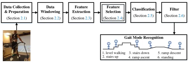
In this section, we present the methodology used to design the UIR system. The architecture of the 105
UIR system is illustrated in Figure1. Our new contribution is a novel feature selection method based 106
on MOO, as illustrated in Figure1in the double-lined box (Section2.4). In this box, the application of 107
four MOBBO methods for gait mode classification is new, and a novel MOO-based feature selection 108
method called GMOFS is new. The remaining parts of the UIR system are implemented based on the 109
existing literature. The role of each subsystem is explained in more detail in the following subsections. 110
Data Collection & Preparation
(Section 2.1)
Data Windowing
(Section 2.2)
Feature Extraction
(Section 2.3)
Classification
(Section 2.5) Feature
Selection
(Section 2.4)
Filter
(Section 2.6)
1. level walking 2. stairs up
3. stairs down 4. ramp ascent
5. ramp descent 6. standing Gait Mode Recognition
1 2 3 4 5 6
Figure 1. Architecture of user intent recognition system. The double-lined box indicates that an evolutionary algorithm is used for optimization.
2.1. Data Collection and Preparation 111
Data collection can significantly affect the accuracy of UIR. Input signals must be informative 112
enough to accurately discriminate between various human gait modes. Four types of input data are 113
four types include signals that reflect: (1) the state of the prosthesis, (2) the state of the residual limb, 115
(3) the user-prosthesis interaction, and (4) the prosthesis-environment interaction. 116
In this paper, we collect vertical hip position and thigh angle to indicate the state of the residual 117
limb, and hip moment to indicate the user-prosthesis interaction. These signals are like an implicit 118
communication link between the user and the prosthesis and can be used to infer user intent. Based 119
on Nyquist’s sampling theorem, measurement signals are sampled at 100 Hz, a frequency that is 120
significantly higher than that of human walking [31]. Then the signals are filtered to eliminate noise 121
and to handle missing measurement data points [32]. Missing data points are recovered with basic 122
interpolation methods. 123
2.2. Data Windowing 124
To effectively classify human gait modes, we extract appropriate features from a frame (window) 125
of measurement signals. Frame lengthLf defines the number of samples in a frame. A short frame
126
fails to provide a rich data set and may lead to significant classification bias and variance. On the other 127
hand, a long frame is a computational burden for real-time implementation. In this paper,Lf is chosen
128
to trade off feature richness and computational load. 129
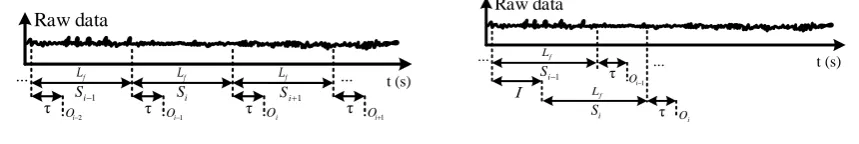
We apply two different methods for data windowing: disjoint windowing and overlapped windowing [33]. Figure2illustrates the two windowing approaches. In disjoint windowing, the class outcomeOicorresponding to frameSiis output everyLf ms.τis the time required for feature extraction, classification, commanding the appropriate low-level controller, and prosthesis response time. In overlapped windowing, we use a sliding frame with lengthLf and incrementI, and the class
outcome is output everyIms. Disjoint windowing is a special case of overlapped windowing when I=Lf. To achieve real-time operation, the parameters of the windowing approaches should satisfy
τ≤Lf disjoint windowing
τ≤ I≤Lf overlapped windowing
(1)
In this paper, we apply disjoint and overlapped windowing with various frame and increment 130
lengths. We consider two important characteristics to determineLf [33]: (1) the minimum interval
131
between two distinct muscle contractions is 200 ms [34], and (2) the delay between user intent and the 132
resultant prosthesis motion should be no more than 300 ms [35,36]. The first property implies that a 133
200 ms frame of data should have the potential to provide rich features for gait mode classification. The 134
second property, which is known as the real-time constraint, ensures that the amputee will experience 135
the prosthesis as responsive to his or her intent. The real-time constraint requiresτ≤Lf ≤300 ms
136
for disjoint windowing, andI≤300 ms for overlapped windowing. Therefore, we use overlapped 137
windowing when the frame length is larger than 300 ms, noting that a larger frame will require a 138
higher computational load.
Raw data
t (s)
... ...
1
i
S Si Si1
2
i
O τ Oi1 τ Oi τ Oi1
τ
f
L
f
L
f
L
(a)Disjoint windowing
Raw data
t (s)
I
τ
... ...
1 i S
i S
1
i
O
i O τ
f
L
f
L
(b)Overlapped windowing
Figure 2.Data windowing.Sirepresents thei-th data segment,Lf is the frame length,τis the required
processing time,Iis the increment length for overlapped windowing, andOiis the detected gait mode
corresponding to frameSi.
2.3. Feature Extraction 140
Various features can be extracted from a frame of measurement data and used for classification. 141
Features should be rich enough to discriminate between various gait modes. In addition, feature 142
extraction needs to be computationally fast for real-time implementation. In general, both time-domain 143
(TD) and frequency-domain (FD) features are frequently used for classification [33,37,38]. We compare 144
TD and FD features in this paper, and select the optimal subset of features for UIR. 145
TD features are computationally fast, and include information about the data waveform and 146
frequency. We extract the following TD features from each frame of data: slope sign change (SSC), zero 147
crossing (ZC), waveform length (WL), variance (VAR), mean absolute value (MAV), modified MAV, 148
root mean square (RMS), Willison amplitude (WAMP), skewness (SK), kurtosis (KU), and correlation 149
coefficient (COR) and angle (ANG) between two frames of data from different measurement signals. 150
In addition, multiple FD features have been extracted. FD features are computationally slower 151
than TD features, but include information about the frame’s frequency content. We use periodograms 152
to measure the power spectrum density (PSD) of a frame, and calculate the following FD features: 153
mean frequency (MNF), median frequency (MDF), maximum frequency (MAXF), and fourth-order 154
auto-regressive coefficients (AR4). 155
Previous research has shown the applicability of these TD and FD features for prosthetic limb 156
pattern recognition [37–39]. Therefore, we are motivated to investigate the performance of these 157
features for gait mode recognition. The mathematical definitions of these TD and FD features are given 158
in [37]. 159
After extracting TD and FD features from a frame of measurement data, the features are 160
concatenated and labeled to create a single training pattern. For instance, extraction of VAR, 161
MAV + RMS, and AR4 features from a frame of three measurement signals (e.g., vertical hip position, 162
thigh angle, and thigh moment) would produce a training vector with 3, 6, and 12 elements, respectively. 163
We perform the above procedure for all features and all frames of measurement data to create the 164
training data set. The training set is then normalized to equalize the relative magnitude of each feature. 165
2.4. Feature Selection 166
The objective of feature selection is to find a subset of the features that were obtained with the 167
feature extraction method. The feature selection method attempts to find a parsimonious feature subset 168
that results in accurate classification. However, subset size and classification accuracy are conflicting 169
objectives. A small feature subset will probably result in high classification error, whereas a large 170
feature subset will probably result in lower classification error. Therefore, feature selection can be 171
viewed as an MOO problem. In MOO problems, no single solution can simultaneously optimize all 172
objectives. The solutions comprise a set of possible alternative solutions known as the optimal Pareto 173
set [20]. 174
We seek the most informative but parsimonious subset of features for gait mode classification. 175
Note that exhaustive search is not practical in cases with a high-dimensional set of features. A set 176
ofnfeatures has 2n different subsets. Many heuristic search strategies, such as sequential forward 177
selection, sequential backward elimination, and evolutionary search, have been suggested for this 178
type of combinatorial problem [40]. EAs have been demonstrated as an efficient search strategy for 179
feature selection [41]. In this section, we propose a search strategy based on BBO, in addition to a 180
new gradient-based algorithm, to solve the MOO problem. We then use two systematic approaches to 181
compare the performance of the different search strategies. 182
2.4.1. Biogeography-Based Multi-Objective Optimization 183
and 0 indicates otherwise. Therefore, each individual in the MOO algorithm is a binary sequence with length equal to the problem dimension. We evaluate the following two objective functions for all individuals in the population.
f1i =number of selected features in thei-th individual
f2i =average prediction error usingc-fold cross validation
(2)
wherei=1,· · ·,N, andNis the population size. We combine BBO with four MOO algorithms [20] to 184
obtain VEBBO, NSBBO, NPBBO, and SPBBO. We apply these MOBBO variants to find the optimal 185
Pareto set for the optimization problem. We investigate the performance of each method in a later 186
section. 187
Although it is possible to use any classification algorithm, we use LDA to compute f2i. LDA, 188
unlike other learning algorithms such as MLP, does not require time-consuming iterations to build a 189
model. This point is important because EAs require many objective function evaluations to find the 190
solution. It is possible to use either classification accuracy or error as the quality measure for the second 191
objective. We use average classification error ofc-fold cross validation (CV). Inc-fold CV, we randomly 192
divide the training set intocdistinct folds. Then we repeat trainingctimes; each time the model is 193
trained usingc−1 folds and is tested with the remaining fold. The average of thecclassification errors 194
is used as the quality measure. 195
2.4.2. Gradient-Based Multi-Objective Feature Selection 196
Although MOBBO and other gradient-free MOO methods have the potential to find the globally 197
optimal solution [21,22], they are computationally expensive due to the need for many iterations of 198
the classifier training process (multiple individuals in the population, and multiple generations). To 199
reduce computational complexity, we propose a novel algorithm called GMOFS for feature selection. 200
In GMOFS, feature selection and data classification are performed simultaneously. 201
GMOFS incorporates a regularization penalty term to the optimization problem of its learning algorithm. The penalty term, which is handled by a Lagrange multiplier, directs the trained model toward a parsimonious as well as accurate model. We use an MLP network as the classifier, and include an elastic net to penalize the size of the selected feature subset. The first step of GMOFS is to train a constrained MLP network with the cost function
J= 1
2
m
∑
l=1
K
∑
j=1
t(jl)−o(jl)2+λ n
∑
i=1
αβ2i + (1−α)|βi|
(3)
whereβiis the multiplier of thei-th input feature before input to the MLP network;tj(l)ando(jl)are the
target and actual value, respectively, of thej-th output neuron associated with thel-th training pattern; Kis the number of output neurons (classes);mis the number of training patterns; andnis the number of input features. We use an MLP network with one hidden layer andphidden neurons (including the bias node).vihdenotes the weight that connects thei-th input neuron to theh-th hidden neuron,
andwhjdenotes the weight that connects theh-th hidden neuron to thej-th output neuron. The first
term of the cost function penalizes classification error while the second term, which is the elastic net, penalizes the number of selected features. The elastic net is a convex combination of ridge regression (α=1) and least absolute shrinkage and selection operator (α=0). λ≥0 is a complexity parameter that controls the shrinkage of the input features. Largeλleads to a shrinkage ofβitoward zero, which
implies that the input feature corresponding toβiis not significant. However, as shrinkage increases,
the number of selected features. In summary, the construction of the MLP network with the elastic net is formulated as the following optimization problem:
min
β,w,v
J subject to (
0≤βi ≤1
|whj| ≤aand|vih| ≤b (4)
for alli,j,h, whereβi =0 or 1 implies that the associated feature is the least or most significant input
variable, respectively. However, due to the direct relationship betweenβiand neuron weightsvihand
whj, we cannot conclude that an input feature with smallβiand large neuron weights is insignificant.
To avoid optimization solutions with large weights, neuron weights are constrained. Backpropagation is used to update βi,vih, andwhj. The derivative of Jwith respect to output weights whj, hidden
weightsvih, and input weightsβiis obtained by the chain rule as
∂J ∂whj
= m
∑
l=1 δ(jl)y(hl)
∂J ∂vih
= m
∑
l=1
∑
k∈D2(h)
h δk(l)whk
i
yh(l)(1−yh(l))βix(il)
∂J ∂βi
= m
∑
l=1
s∈
∑
D1(i)
∑
k∈D2(h)
h δ(kl)wsk
i
y(sl)(1−y(sl))vis
x (l) i
+λ
2αβi+ (1−α) βi |βi|
(5)
whereD1(i)is the set of middle layer neurons whose inputs come from thei-th input neuron,D2(h) 202
is the set of output neurons whose inputs come from the h-th middle layer neuron, andδj(l) = 203
−(o(jl)−t(jl))(1−t(jl))t(jl). We use the derivatives in Eq.5and constraints in Eq.4along with the trust 204
region reflective algorithm to train the constrained MLP network. 205
Once MLP training phase is completed, input weightsβi are sorted in descending order. The
input variable with the largestβiis the most significant feature. The second step of GMOFS is to select
the mostrsignificant features, which are associated with therlargest input weightsβi, and which
satisfy
∑r
i=1βi
∑n
j=1βj
≥95%
β1≥β2≥ · · · ≥βn
(6)
We then repeat the first two steps of GMOFS for differentλin the range[λl,λu]with a predefined
increment4λ. The selected subsets associated with eachλcomprise a population. The population size depends on4λ. To assess the performance of the selected feature subset, we train a classifier with each selected subset and find classification error. In this population, the subset associated withλ→∞ has minimum size and maximum classification error, whereas the subset withλ=0 has maximum size and probably has the lowest classification error. Thus, the size of the selected subset and the classification error, defined in Eq.2, are two conflicting objectives. To find the GMOFS Pareto front, we first obtain the Pareto set as
Ps =
x∗:h@x: fi(x)≤ fi(x∗)for alli∈[1, 2], and fj(x)< fj(x∗)for somej∈[1, 2] i
(7)
x∗denotes the set of non-dominated solutions in the population and fi(x)is thei-th objective function.
The Pareto frontPf is obtained from all function vectors f(x)that correspond to the Pareto set:
Note that all Pareto points are equally preferable apart from subjective prioritization. The outline of 206
GMOFS is given in Algorithm1. 207
Algorithm 1The outline of gradient-based multi-objective feature selection (GMOFS), wherexiis the
i-th feature in the training setX, andYis the corresponding set of output classes.
Initialization:λ=λl≤λu, Population =∅,k=1 Whileλ≤λu
Step 1:
Use the training data{X,Y}to train the constrained MLP network in Eq.3by solving Eq.4 Step 2:
Sort the input weights{βi}in descending order
Use Eq.6to select subsetSk⊂Xwhere size(Sk)≤size(X) Step 3:
Population←Population+Sk
k←k+1 Nextλ←λ+4λ Step 4:
Foreach subsetSkin Population
Use cross-validation to train and test a classifier with dataset{Sk,Y}
Calculate objective functions f1kand f2kusing Eq.2 NextsubsetSk
Step 5:
Find the Pareto set using Eq.7
2.4.3. Evaluation of Multi-Objective Optimization Pareto Fronts 208
We will compare the Pareto fronts obtained by each MOO algorithm using normalized hypervolume and relative coverage. These methods are popular for evaluating the quality of a Pareto front. The Pareto front normalized hypervolume is computed as follows:
Normalized Hypervolume= ∑ Np
j=1∏
M i=1fji
Np (9)
whereMis the number of objectives, fjiis the value of thei-th objective function of thej-th Pareto
209
point, andNpis the number of Pareto points.
210
Another way to compare Pareto sets is to compute the coverage of one Pareto set relative to a 211
second Pareto set. This metric is determined by the number of solutions in the first Pareto set that 212
are weakly dominated by at least one solution in the second Pareto set [20]. A smaller number for 213
normalized hypervolume and relative coverage indicates better performance. 214
2.5. Classification 215
Accurate classification of gait patterns is the ultimate goal of the UIR system. For this purpose, 216
we assess various well-known linear and non-linear classification techniques, including LDA, QDA, 217
SVM, DT, and MLP classifiers. 218
LDA and QDA classifiers do not require time-consuming iterations for training. In fact, the 219
parameters of these classifiers are directly obtained from the training data. Although these classifiers 220
are fast in terms of training, they are not as flexible as nonlinear classifiers such as SVM, DT, and MLP. 221
These classifiers solve an optimization problem that minimize the classification error. In most cases, 222
it is difficult to find optimization solutions in closed form, so we use either iterative optimization 223
We use one-against-one approach to implement multi-class SVM, and we also evaluate the 225
performance of different kernels, such as linear and RBF. We tune the parameters of the SVM kernels to 226
achieve the best classification performance. To increase the accuracy of the MLP network, we perform 227
a grid search of the number of hidden nodespfrom the set{3, 4, 5, 6, 8, 10, 15, 20}, and we measure 228
the mean classification error using five-fold CV. Then we choose p to obtain a trade-off between 229
classification accuracy and classifier complexity. An MLP with smallpmay not result in the desired 230
accuracy, but an MLP with large pmay tend to memorize the noise in the training set and lead to 231
overfitting and poor generalization. In addition, we use Wilcoxon signed-rank tests to statistically 232
compare the classification methods. 233
2.6. Filter 234
To enhance the prediction performance of the UIR system, we incorporate a majority voting 235
filter (MVF). MVF alleviates transient jumps between classifier output classes and leads to smooth 236
transitions from one classified gait mode to another . We implement the MVF using 2q+1 classified 237
modes [39]: the current,qprevious, andqsubsequent values. The MVF output is the most frequently 238
classified mode among those 2q+1 values. 239
Since MVF uses q future classified gait modes to calculate the current classified mode, an inappropriate value forqmay violate the real-time constraint. The constraint requires that the classified mode is output with a time delay less than 300 ms (see Section2.2). The constraint requires
q×Lf ≤300 ms Disjoint windowing
q×I ≤300 ms Overlapped windowing (10)
An MVF with very smallqmay not significantly improve classification performance, whereas an MVF 240
with very largeqmay cause misclassification because of time delay. In this paper, we will choose a 241
trade-off value forq, and will investigate the effect of the MVF on classification performance. 242
3. Results and Discussion 243
This section evaluates the performance of the UIR system and its subsystems as discussed in 244
Section2. 245
3.1. Experimental Setup and Data Collection 246
To design and evaluate the performance of the UIR system, we collect data from three able-bodied 247
subjects (AB01, AB02, and AB03) and three transfemoral amputee subjects (AM01, AM02, and AM03). 248
All the experiments were approved by the Department of Veterans Affairs Institutional Review Board. 249
The above-knee amputees wore an Ottobock prosthesis on the right leg. As discussed in Section2.1, 250
we measure vertical hip position, thigh angle, and thigh moment for UIR. These signals are collected 251
for able-bodied subjects during four different activity modes: (1) standing (ST), (2) normal walking 252
(NW) at user-preferred speed (PS), (3) slow walking (SW), and (4) fast walking (FW). Due to physical 253
limitations, we collect data during only three activity modes for the amputee subjects: ST, NW, and 254
SW. Table1shows the physical characteristics of the subjects. 255
The data were collected at the Motion Study Laboratory of the Cleveland Department of Veterans 256
Affairs Medical Center with 47 reflective markers on each subject’s body. Subjects were asked to walk 257
on a treadmill with built-in force sensors. A 16-camera Vicon system recorded kinematic data at 100 Hz. 258
Ground reaction force along three axes were collected from the force sensors at 1000 Hz. Data were 259
filtered with a second-order low-pass filter with a cutoff frequency of 6 Hz. Filtered data were input to 260
inverse dynamics software to calculate the joint angles and torques. Detailed methods and sample 261
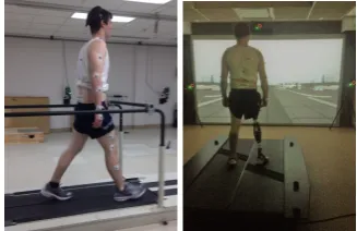
results can be found in [32]. The experimental setup is illustrated in Figure3. Note that the lower-limb 262
amputee demographic at the Veterans Affairs Medical Center, where data collection was performed, 263
Table 1.Physical characteristics of the six human test subjects. AB and AM represent able-bodied and amputee subject, respectively.
Gender Age Weight Height Walking Speed (m/s)
(years) (kg) (cm) SW PS FW
AB01 Male 37 79.5 188 0.98 1.30 1.63
AB02 Male 20 73.9 172 0.86 1.15 1.44
AB03 Male 28 80.9 179 0.75 1.00 1.25
AM01 Male 32 79.1 174 0.60 1.00 –
AM02 Male 64 99.2 177 0.56 0.94 –
AM03 Male 35 81.7 176 0.60 0.90 –
Our future work will need to include more subjects and wider demographics (for example, ages and 265
genders). 266
Figure 3.Experimental setup for data collection. The left figure shows an able-bodied subject and the right figure shows an amputee subject with an Ottobock prosthesis on the right leg.
Note that in a real-world, non-laboratory settings, we would measure the required input signals 267
directly rather than with cameras. For example, we could use piezo-electric sensors or multi-axis 268
load cells for force sensing, and optical encoders or inertial measurement units for position and angle 269
sensing [11]. 270
The able-bodied subjects were asked to perform four sequences of walking trials, each lasting 271
approximately 60 seconds. Each sequence consists of four different gait modes (ST, SW, NW, and FW) 272
and each mode was maintained for several seconds. Figure4illustrates a sample walking trial for 273
AB01. The amputee subjects performed six sequences of three different walking modes, each lasting 274
approximately 30 seconds. 275
In summary, we note a few important points. Firstly, in this paper, the type of walking activities 276
used for recognition is not our main focus, but rather the assessment of the proposed methodology 277
to eliminate irrelevant/redundant features for UIR is our main goal. Secondly, in human activity 278
mode recognition applications, an entire stride is typically used for non-real-time classification [43]. 279
However, in UIR, we use a small window of measurement signals, mostly within a few milliseconds, 280
to identify user’s intent for real-time prosthesis control. 281
3.2. Effect of Frame Length on Classification Performance 282
The objective of this section is to choose the appropriate data windowing method and frame 283
length. We investigate the influence of disjoint and overlapped windowing with different frame 284
lengths on the classification accuracy of the UIR system. We use disjoint windowing with frame lengths 285
Lf ={100, 150, 200, 250}ms, and overlapped windowing with frame lengthsLf ={200, 250, 300}ms
286
and incrementsI={50, 150, 200}ms. We extract TD and FD features from the data frames generated 287
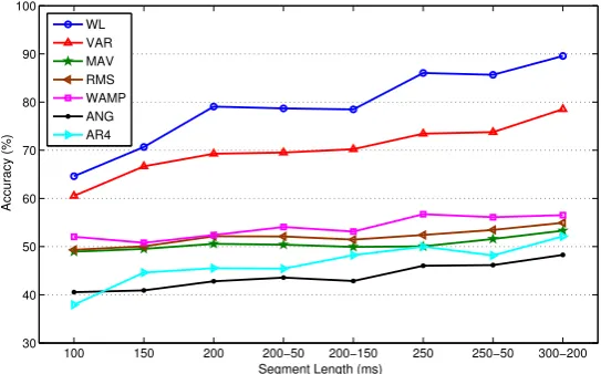
by the three measurement signals collected from able-bodied subjects. Figure5shows the mean 288
classification performance of LDA with different frame lengths. Note that the size of the dataset 289
depends on the parameters of the windowing methods. For instance, a 10-second walking sequence 290
0.9 0.92 0.94 0.96
Hip Vertical Position (m)
−10 0 10 20 30
Hip Flexion Angle (deg)
−150 −100 −50 0 50
Hip Moment
(Nm)
0 10 20 30 40 50 60
ST SW NW FW
Activity Modes
Time (sec)
Figure 4.Sample walking trial with four different gait modes for able-bodied subject AB01
In this experiment, LDA is separately trained and tested using 10-fold CV for each subject 292
with only one feature type for each of the measurements: WL, VAR, MAV, RMS, WAMP, ANG, 293
and AR4. These features are used because they are considered the most representative TD and FD 294
features. Figure5illustrates the mean classification accuracy of LDA for the two able-bodied subjects 295
using 10-fold CV. A single value on the horizontal axis of the figure indicates the frame length of 296
disjoint windowing. A pair of values indicates the frame length and increment length of overlapped 297
windowing; for instance, 200−50 denotesLf =200 ms andI=50 ms.
298
Figure5shows that the classification accuracy typically improves as the frame length increases. A 299
larger frame is more likely to include richer information, and consequently lower bias and variance 300
in classification performance. For instance, the increase in accuracy with WL is approximately 19% 301
when the frame length increases from 100 ms to 200 ms. The increases are 14.3% and 16% when 302
using the VAR and AR4 features, respectively. However, the accuracy does not vary significantly with 303
frame length for the remaining features in Figure5. The figure illustrates that all representative TD 304
features except ANG provide better classification performance than AR4, which is the representative 305
FD feature. 306
In this experiment, very small frame length is not used because it would result in poor prediction 307
accuracy. Conversely, large frame length is not used because it would result in a violation of the 308
real-time constraint. To find the best frame length, we statistically compare performance using 309
100 150 200 200−50 200−150 250 250−50 300−200 30
40 50 60 70 80 90 100
Segment Length (ms)
Accuracy (%)
WL VAR MAV RMS WAMP ANG AR4
Wilcoxon signed-rank tests. For this purpose, LDA is trained using only one TD or FD feature at 310
a time. The null hypothesis of the test is that the differences between mean classification accuracy 311
corresponding to two different frame lengths are from a distribution with zero mean at the specified 312
level of significance. If the null hypothesis cannot be rejected, then we conclude that the two compared 313
frame lengths are not statistically significantly different, as indicated by an≈sign and a T (tie). If we 314
can reject the null hypothesis, then the two frame lengths are statistically significantly different, and 315
this is indicated by a+sign. The better frame length is the one with better mean classification accuracy 316
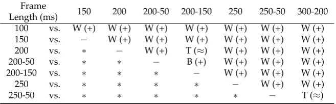
and is shown by B (better) while the worse one is shown by W (worse). Table2provides the results of 317
the statistical tests at a 10% significance level. 318
Table2shows that frames with length larger than 200 ms perform better than frames with length 319
150 or 100 ms. Table2shows that the two overlapped frame windows withLf =250 ms,I=50 ms
320
andLf =300 ms,I =200 ms tie for similar performance, and perform better than the other frame
321
lengths. 322
Taking into account the real-time constraint, the length of the MVF filter, and processing time, we 323
choose overlapped windowing withLf =250 ms,I=50 ms throughout the remainder of the paper as
324
the best trade-off, except where specifically mentioned otherwise. 325
Table 2. Comparison of classification performance for different frame lengths (row values versus column values) using Wilcoxon signed-rank tests at a 10% significance level.≈indicates that the two compared frame lengths tie (T) with similar performance and are not statistically significantly different. +indicates that the two frame lengths are statistically significantly different, and B or W indicates that
the row frame length performs better or worse than the column frame length, respectively.
Frame
Length (ms) 150 200 200-50 200-150 250 250-50 300-200 100 vs. W (+) W (+) W (+) W (+) W (+) W (+) W (+)
150 vs. − W (+) W (+) W (+) W (+) W (+) W (+)
200 vs. ∗ − W (+) T (≈) W (+) W (+) W (+)
200-50 vs. ∗ ∗ − B (+) W (+) W (+) W (+)
200-150 vs. ∗ ∗ ∗ − W (+) W (+) W (+)
250 vs. ∗ ∗ ∗ ∗ − W (+) W (+)
250-50 vs. ∗ ∗ ∗ ∗ ∗ − T (≈)
We use principal component analysis (PCA) [44] and Fisher linear discriminant analysis 326
(FLDA) [45] to visualize the training set. A training pattern is a vector of all TD and FD features 327
extracted from a frame of raw data. We performed 2D dimension reduction for three different frame 328
lengths. Figure6illustrates the 2D scatter plot for able-bodied subject AB01. To save space, we do not 329
provide the same figures for other subjects because we obtained similar results for those subjects. 330
Figure 6 shows that FLDA provides better visualization than PCA in terms of gait mode 331
separability. We verify that longer frame length leads to better gait mode separation, and eventually 332
better classification performance. Most importantly, Figure6verifies the effectiveness of the TD and 333
FD features. 334
3.3. Multi-Objective Feature Selection 335
We perform feature selection in two steps. In the first step we exclude non-informative TD and FD 336
features, and in the second step we use MOO to further refine the selected feature set. We implement 337
five different MOO methods, including our newly proposed method, to find the optimal set of features. 338
The complete set of features includes the following TD and FD features: SSC (F1), ZC (F2), WL (F3), 339
VAR (F4), MAV (F5), MAV1 (F6), MAV2 (F7), RMS (F8), WAMP (F9), SK (F10), KU (F11), FMD (F12), FMN 340
(F13), FMAX (F14), COR (F15), ANG (F16), and AR4 (F17). We perform preliminary feature selection 341
using two able-bodied subjects. We use MOO for final feature selection using only one able-bodied 342
subject to reduce computational effort. Later we will investigate the performance of the selected 343
−2 −1 0 1 2 −5
0 5
2nd PC
x FW o NW
+ SW* ST
−10 −5 0 5
−8 −6 −4 −2 0 2 4
2nd Discriminant Disjoint window (L f = 100 ms)
−6 −4 −2 0 2 4 6
−5 0 5
2nd PC
Disjoint window (L f = 100 ms)
Disjoint window (Lf = 250 ms)
−10 −5 0 5
−5 0 5
2nd Discriminant
Disjoint window (Lf = 250 ms)
−5 0 5
−5 0 5
1st PC
2nd PC
Overlapped window (Lf = 500 ms, I = 200 ms)
−15 −10 −5 0 5
−10 −5 0 5
1st Discriminant 2nd Discriminant Overlapped window (L
f = 500 ms, I = 200 ms)
Figure 6.Two-dimensional scatter plot for visualization using PCA (left column) and FLDA (right column) for able-bodied subject AB01
In the first step, we train LDA for each of two able-bodied subjects, and separately for each 345
individual feature type listed in the previous paragraph, using 10-fold CV for each training procedure. 346
The mean classification accuracy over the two subjects and the ten folds are used to assess the 347
importance of each feature type. Since we need to train the classifier several times in this step, we 348
choose to use LDA due to its fast training time. 349
Figure7 shows the mean classification accuracy and processing ratio for each feature type. 350
Processing ratio indicates the relative computational complexity to compute each feature type. Figure7
351
indicates that TD features require less computational effort than FD features. For instance,F12,F13, and 352
F14require high computational effort compared to other features. We excludeF12,F13, andF14from 353
the candidate feature set due to their relatively high computational expense and poor classification 354
accuracy. In addition,F6andF7, two variants of MAV, are excluded due to their poor classification 355
accuracy and because they provide information that is similar to MAV. Therefore, we exclude a total of 356
five weak feature types, and pre-select the remaining 12 feature types. This results in a training vector 357
with 11×3+4×3=45 elements. Note that the AR4 feature type includes four components and thus 358
contributes a total of 12 elements from the three measurement signals. Finally, vertical hip position 359
does not cross zero (see Figure4), thus the ZC feature of this signal is excluded. In summary, we have 360
a training data set with 44 features. 361
Now we are ready to proceed to the feature selection step. In this step we use VEBBO, NSBBO, 362
NPBBO, SPBBO, and GMOFS to select an optimal subset from the 44 pre-selected features. To reduce 363
the computational expense, we use only the AB01 training data set in this step. We then verify that the 364
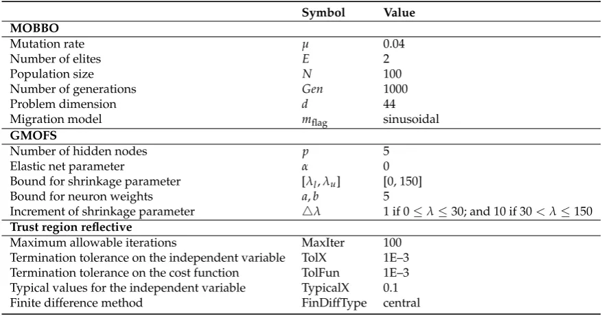
selected subset results in a satisfactory UIR system when trained for other subjects. Table3shows the 365
tuning parameters used in this paper. To tune the parameters, we performed a sensitivity analysis of 366
MOO performance to each parameter, one at a time, to find a local optimum of MOO performance with 367
respect to each parameter. For instance, GMOFS is implemented with different elastic net parameter 368
valuesα= {0, 0.5, 1}, and we found that the Pareto front withα =0 dominates Pareto fronts that 369
are found with other values ofα. For training the neural network in GMOFS, we used the MATLAB 370
function fmincon from the Optimization Toolbox to implement a trust region reflective algorithm. We 371
mostly used default values for the fmincon parameters, but we found that the performance of GMOFS 372
is not very sensitive to these parameters. 373
We run each multi-objective method for 10 independent trials, and the best Pareto front of each 374
F1 F2 F3 F4 F5 F6 F7 F8 F9 F10 F11 F12 F13 F14 F15 F16 F17 0
20 40 60 80 100
Features
Accuracy (%)
0 20 40 60 80 100
Processing Ratio (%)
Accuracy Processing Ratio
4.22 2.95 0.32 1.66
2.10 0.54 0.13 1.11 0.94 0.09 0.24 0.24 0.52 0.67
Figure 7.Mean classification accuracy over two able-bodied subjects, and processing ratio of 17 feature types trained by LDA using 10-fold cross validation
Table 3.Tuning parameters for multi-objective feature selection
Symbol Value MOBBO
Mutation rate µ 0.04
Number of elites E 2
Population size N 100
Number of generations Gen 1000
Problem dimension d 44
Migration model mflag sinusoidal
GMOFS
Number of hidden nodes p 5
Elastic net parameter α 0
Bound for shrinkage parameter [λl,λu] [0, 150]
Bound for neuron weights a,b 5
Increment of shrinkage parameter 4λ 1 if 0≤λ≤30; and 10 if 30<λ≤150
Trust region reflective
Maximum allowable iterations MaxIter 100
Termination tolerance on the independent variable TolX 1E–3 Termination tolerance on the cost function TolFun 1E–3 Typical values for the independent variable TypicalX 0.1
Finite difference method FinDiffType central
significantly dominates all four MOBBO Pareto fronts. However, we are aware of the fact that MLP, 376
which is used in GMOFS, generally outperforms LDA, which is used in the MOBBO variants, for 377
complicated nonlinear problems. 378
To have a more fair comparison, we apply SVM with linear kernels to all of the optimal feature 379
subsets found by the MOO methods. Figure8(a) illustrates the Pareto fronts obtained by the five 380
MOOs with SVM with linear kernels. Figure8(a) shows that the Pareto fronts of VEBBO, SPBBO, 381
NSBBO, and GMOFS are close, and clearly dominate the NPBBO Pareto points. Figure8(b) indicates 382
the combined Pareto front obtained from all of the non-dominated points in Figure8(a). GMOFS 383
provides the maximum contribution to the combined Pareto front, while NPBBO does not contribute 384
any Pareto points. All of the points in Figure8(b) are labeled for easy referencing. 385
To systematically compare the Pareto fronts in Figure 8(a), we use relative coverage and 386
normalized hypervolume as discussed in Section2.4.3. Tables4and5provide the comparison results 387
using these two approaches. In Table4, an entry in columniand rowj(i6=j) indicates the percentage 388
of Pareto points of the method of columnithat is dominated by at least one Pareto point of the method 389
5 10 15 20 25 30 1.0
1.5 2.0 2.5 3.0 3.5 4.0 4.5 5.0
f1: Number of features
f2
: Classification error (%)
VEBBO SPBBO NSBBO NPBBO GMOFS
(a)
5 10 15 20 25
1.0 1.5 2.0 2.5 3.0 3.5 4.0 4.5 5.0
f1: Number of features f2
: Classification error (%)
VEBBO SPBBO NSBBO GMOFS p1
p2
p4 p3
p5 p6
p7 p8
p9
p10 p
12
p
11
(b)
Figure 8.(a) Pareto fronts obtained from MOO methods with an SVM classifier with linear kernels using AB01 training data; (b) combined Pareto front obtained from non-dominated Pareto points in (a).
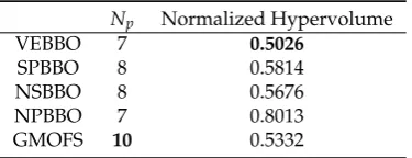
at least one Pareto point from the other four MOO methods. Therefore, VEBBO ranks first in terms 391
of relative coverage. GMOFS ranks second and performs better than SPBBO, NSBBO, and NPBBO. 392
In addition, Table5shows that VEBBO and GMOFS rank first and second in terms of normalized 393
hypervolume, respectively. GMOFS ranks first in terms of the number of Pareto points. These results 394
verify the competitive performance of GMOFS compared to the other four MOO methods. 395
Most importantly in terms of the advantage of GMOFS, it requires the execution of only 43 396
classifier training procedures (due to the number of λincrements), while each of the other four 397
EA-based MOO methods require 100,000 training procedures (due to the combination of population 398
size and generation limit). 399
Table 4.Comparison of Pareto fronts using relative coverage (RC). Only 7.2% and 30% of the VEBBO and GMOFS points, respectively, are dominated by other Pareto points; so VEBBO and GMOFS rank first and second, respectively, in terms of RC.
VEBBO SPBBO NSBBO NPBBO GMOFS
VEBBO − 62.5 75.0 85.7 40.0
SPBBO 0.0 − 25.0 71.4 40.0
NSBBO 14.3 50.0 − 100.0 40.0
NPBBO 0.0 0.0 0.0 − 0.0
GMOFS 14.3 50.0 50.0 100.0 −
Mean RC(%) 7.2 40.4 37.5 89.3 30.0
Table 5. Comparison of Pareto fronts using normalized hypervolume. Npis the number of Pareto
points obtained by each MOO method. VEBBO and GMOFS rank first and second, respectively, in terms of normalized hypervolume, and GMOFS ranks first in terms of the number of points.
Np Normalized Hypervolume
VEBBO 7 0.5026
SPBBO 8 0.5814
NSBBO 8 0.5676
NPBBO 7 0.8013
GMOFS 10 0.5332
The benefit of presenting the data of Figure8(b) is that it allows us to find the best subset of 400
features for an accurate and parsimonious classifier. Among the 12 Pareto points, we choosep9as 401
on the priority of the problem objectives, but p9 provides a good trade-off between classification 403
error and number of features. Therefore, in Section3.5we will investigate classification performance 404
with candidate solutionp9for all human subject data AB01, AB02, AB03, AM01, AM02, and AM03. 405
However, first we will find the best classifier in the following section. 406
3.4. Comparison Results of Classification Algorithms 407
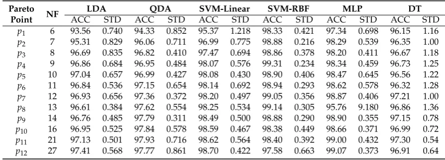
In this section, we use p1 through p12 to statistically compare the performance of different 408
classifiers for subject AB01. The objective is to find the best classifier for locomotion mode detection 409
among LDA, QDA, SVM with linear kernels (SVM-linear), SVM with RBF kernels (SVM-RBF), MLP, 410
and DT. The tuned parameter value of RBF kernel isσ=1. Table6shows mean classification accuracy 411
and standard deviation of each classifier trained with the features from each Pareto point using 10-fold 412
CV. 413
Table7presents pair-wise statistical comparisons using Wilcoxon signed-rank tests at a 5% 414
significance level. If a pair-wise p-value is less than 0.05, the mean performances of the two classifiers 415
are statistically significantly different, and the classifier with larger mean prediction accuracy performs 416
better than the other one. A pair-wise p-value greater than 0.05 indicates no significant difference 417
between the performance of the two classifiers. Table7shows that the classification performance 418
of MLP and SVM-RBF are statistically equal, and are significantly better than the other methods. 419
SVM-linear is statistically better than LDA, QDA, and DT. QDA performs better than LDA and 420
similarly to DT. In summary, MLP and SVM-RBF are the best, SVM-linear is the second best, QDA and 421
DT are the third best, and LDA is the worst for locomotion mode detection. 422
Table 6. Mean classification accuracy (ACC) and standard deviation (STD) for AB01 of classifiers trained with 13 different feature subsets. NF is the number of features in each set.
Pareto Point NF
LDA QDA SVM-Linear SVM-RBF MLP DT
ACC STD ACC STD ACC STD ACC STD ACC STD ACC STD
p1 6 93.56 0.740 94.33 0.852 95.37 1.218 98.33 0.421 97.34 0.698 96.15 1.16 p2 7 95.31 0.829 96.06 0.711 96.99 0.775 98.88 0.216 98.29 0.539 96.35 1.00 p3 8 96.69 0.835 96.82 0.410 97.47 0.694 98.86 0.378 98.20 0.411 96.67 1.18 p4 9 96.86 0.684 96.95 0.484 98.07 0.576 99.31 0.234 98.34 0.459 96.73 1.25 p5 10 97.04 0.657 96.99 0.427 98.08 0.430 98.90 0.406 98.47 0.645 96.56 1.22 p6 11 96.84 0.536 97.15 0.654 98.14 0.692 98.94 0.293 98.62 0.578 96.32 1.28 p7 12 96.93 0.656 97.36 0.372 98.20 0.497 99.05 0.356 98.87 0.406 97.21 1.00 p8 13 96.61 0.384 97.62 0.554 98.25 0.534 99.14 0.305 95.76 9.180 96.86 1.36 p9 14 96.76 0.485 97.79 0.311 98.49 0.500 98.88 0.290 98.90 0.355 97.15 0.78 p10 16 96.95 0.525 97.84 0.578 98.59 0.467 98.38 0.449 98.66 0.371 96.99 0.72 p11 21 97.13 0.501 97.93 0.716 98.62 0.564 98.40 0.392 99.00 0.432 97.30 0.54 p12 27 97.41 0.568 97.77 0.861 98.70 0.422 97.58 0.663 99.07 0.373 96.91 0.64
Table 7.Comparison of classification performance using Wilcoxon signed-rank tests (W.T.) at a 5% significance level. B or W indicates that the row method performs better or worse than the column method, respectively, while T shows that they tie with similar performance. These results are obtained using all the data from Table6.
DT SVM-RBF SVM-linear QDA LDA
p-value W.T. p-value W.T. p-value W.T. p-value W.T. p-value W.T.
MLP vs. 2.44E-4 B 7.32E-1 T 8.50E-3 B 5.02E-3 B 2.44E-4 B
DT vs. − 1.23E-4 W 8.20E-3 W 1.33E-1 T 1.70E-1 T
SVM-RBF vs. ∗ − 6.70E-3 B 2.44E-4 B 1.22E-4 B
SVM-linear vs. ∗ ∗ − 1.15E-4 B 1.25E-4 B
3.5. Performance Assessment of Selected Subset 423
In this section we train UIR for all able-bodied and transfemoral amputee subjects with feature 424
subsetp9. All classifiers are trained with three representative methods (SVM-RBF, SVM-linear, and 425
QDA). The RBF kernel tuning parameter isσ=1 andσ=4 for able-bodied and amputee subjects, 426
respectively. In this section, we use multiple-fold CV for learning, where each walking sequence is 427
considered a fold. 428
We saw in Section2.2that overlapped windowing with frame lengthLf =250 ms and increment
429
I=50 ms is the best data window option. For real-time operation, a conservative choice for parameter 430
q = 5 satisfies the constraintq×I ≤ 300 ms. Therefore, we use MVF with length 2×q+1 = 11. 431
Results verify a fast processing time on a standard desktop computer of less than 50 ms, on average, 432
including feature extraction and classification with each of the three classifiers. 433
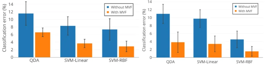
Figure9illustrates the mean classification error of QDA, SVM-linear, and SVM-RBF trained with 434
feature subsetp9. Training was conducted individually for able-bodied subjects AB01, AB02, and AB03 435
and amputee subjects AM01, AM02, and AM03, with and without MVF. Figure9indicates that: (1) 436
SVM-RBF outperforms SVM-linear and QDA, which confirms the statistical results in Section3.4; (2) 437
MVF statistically significantly decreases classification error for locomotion mode detection (p<0.05); 438
and (3)p9is an effective feature subset and results in accurate as well as compact UIR. Feature subset 439
p9uses only 14 features out of a total of 60 available features, which reduces the size of the feature set 440
by 77%. 441
SVM-RBF was also trained for the able-bodied subjects with the full set of 60 features. When 442
combined with MVF it results in a mean classification accuracy of 98.54%±1.92%. In comparison, 443
we achieve 97.14%±1.51% mean classification accuracy with feature subset p9, which includes only 444
14 features. Statistical tests at 5% significance level indicate no significant difference between UIR 445
performance when trained with the full feature set and subsetp9. 446
SVM-RBF was also trained for the amputee subjects with the full set of 60 features. When 447
combined with MVF it results in a mean classification accuracy of 99.37%±0.96%. In comparison, we 448
achieve 98.45%±1.22% mean classification accuracy with feature subsetp9. As with the able-bodied 449
subjects, statistical tests indicate no significant difference between UIR performance when trained with 450
the full feature set and subsetp9. This indicates the satisfactory performance of our framework, which 451
is able to eliminate unneeded features with no significant degradation in overall accuracy. 452
(a)Trained with subsetp9for able-bodied subjects (b)Trained with subsetp9for amputee subjects
Figure 9.Classification performance of QDA, SVM-Linear, and SVM-RBF with feature subsetp9for able-bodied subjects (AB01, AB02, and AB03) and amputee subjects (AM01, AM02, and AM03).
4. Conclusion 453
We presented a framework for designing a UIR system. We used experimental data collected 454
from three able-bodied subjects and three above-knee amputee subjects to classify four and three 455
different gait modes, respectively. Overlapped windowing with frame length 250 ms and increment 456
50 ms provided a good tradeoff between classification performance and real-time computation. Several 457
feature selection in two steps. First, we excluded non-informative features with poor classification 459
performance and high computational effort. Second, we used MOO to find an optimal feature subset 460
from the remaining features to obtain a UIR system that was both parsimonious and accurate. For 461
this purpose, GMOFS, a novel embedded multi-objective feature selection algorithm, was proposed 462
and compared with four evolutionary MOOs on the basis of normalized hypervolume and relative 463
coverage. Classification results confirmed the competitive performance of GMOFS. Several classifiers 464
were trained with the optimal feature subsets that were selected by MOO, and SVM-RBF and MLP 465
were found to be the best classifiers for UIR. The outputs of the classifiers were input to an MVF to 466
improve classification accuracy and chattering between the identified classes. 467
For future work, more above-knee amputee subjects will be involved in data collection and 468
classification. In addition, we will include other daily-life activities such as incline walking, stair ascent 469
and descent, standing and sitting, etc. It is also of great interest to consider other informative features 470
for classification, such as wavelet transform coefficients. Finally, it would be of interest to compare 471
GMOFS with other state-of-the-art MOO methods, and to apply GMOFS to other MOO problems. 472
Author Contributions:Investigation, G.K.; methodology, G.K. and H.M.; project administration, D.S.; resources, 473
H.M.; software, G.K.; writing—original draft preparation, G.K. and H.M.; writing—review editing, D.S.; funding 474
acquisition, D.S. 475
Funding: This research was supported by National Science Foundation grants 1344954 and 1536035, and a 476
Cleveland State University Graduate Student Research Award. 477
Acknowledgments:The authors would like to thank Dr. Elizabeth C. Hardin from Cleveland Veterans Affairs 478
Medical Center who contributed to the experiments of collecting data. 479
Conflicts of Interest:The authors declare no conflict of interest. 480
Abbreviations 481
The following abbreviations are used in this manuscript.
List of acronyms in order of appearance
Acronym Definition Acronym Definition
UIR User intent recognition ZC Zero crossing
MOO Multi-objective optimization WL Waveform length
GMOFS Gradient-based multi-objective feature selection VAR Variance
MOBBO Multi-objective biogeography-based optimization MAV Mean absolute value
SVM Support vector machine RMS Root mean square
RBF Radial basis function WAMP Willison amplitude
MVF Majority voting filter SK Skewness
sEMG Surface electromyography KU Kurtosis
LDA Linear discriminant analysis COR Correlation
QDA Quadratic discriminant analysis ANG Angle
GMM Gaussian mixture model PSD Periodogram spectrum density
ANN Artificial neural network MNF Mean frequency
BBO Biogeography-based optimization MDF Median frequency
VEBBO Vector evaluated BBO MAXF Maximum frequency
NSBBO Non-dominated sorting BBO AR Auto-regressive model
NPBBO Niched Pareto BBO CV Cross validation
SPBBO Strength Pareto BBO AB01 Able-bodied subject 01
EA Evolutionary algorithm AM01 Amputee subject 01
MLP Multilayer perceptron PS Preferred speed
TD Time domain ST Standing
FD Frequency domain NW Normal walking
FLDA Fisher’s linear discriminant analysis SW Slow walking
PCA Principal component analysis FW Fast walking
DT Decision tree SSC Slope sign change
References 483
1. Lawson, B.E.; Varol, H.A.; Huff, A.; Erdemir, E.; Goldfarb, M. Control of stair ascent and descent with a 484
powered transfemoral prosthesis.IEEE Transactions on Neural Systems and Rehabilitation Engineering2013, 485
21, 466–473. 486
2. Khademi, G.; Richter, H.; Simon, D. Multi-objective optimization of tracking/impedance control for a 487
prosthetic leg with energy regeneration. IEEE Conference on Decision and Control, 2016, pp. 5322–5327. 488
3. Sup, F.; Varol, H.A.; Mitchell, J.; Withrow, T.J.; Goldfarb, M. Preliminary evaluations of a self-contained 489
anthropomorphic transfemoral prosthesis. IEEE/ASME Transactions on Mechatronics2009,14, 667–676. 490
4. Tucker, M.R.; Olivier, J.; Pagel, A.; Bleuler, H.; Bouri, M.; Lambercy, O.; del R Millán, J.; Riener, R.; Vallery, 491
H.; Gassert, R. Control strategies for active lower extremity prosthetics and orthotics: a review. Journal of
492
Neuroengineering and Rehabilitation2015,12, 1. 493
5. Huang, H.; Kuiken, T.A.; Lipschutz, R.D. A strategy for identifying locomotion modes using surface 494
electromyography. IEEE Transactions on Biomedical Engineering2009,56, 65–73. 495
6. Zhang, F.; Huang, H. Real-time recognition of user intent for neural control of artificial legs. Myoelectric 496
Control/Powered Prosthetics Symposium, 2011. 497
7. Stolyarov, R.; Burnett, G.; Herr, H. Translational motion tracking of leg joints for enhanced prediction of 498
walking tasks. IEEE Transactions on Biomedical Engineering2018,65, 763–769. 499
8. Hargrove, L.; Englehart, K.; Hudgins, B. The effect of electrode displacements on pattern recognition based 500
myoelectric control. Annual International Conference of the IEEE Engineering in Medicine and Biology 501
Society, 2006, pp. 2203–2206. 502
9. Winkel, J.; Jorgensen, K. Significance of skin temperature changes in surface electromyography.European
503
Journal of Applied Physiology and Occupational Physiology1991,63, 345–348. 504
10. Zachariah, S.G.; Saxena, R.; Fergason, J.R.; Sanders, J.E. Shape and volume change in the transtibial 505
residuum over the short term: Preliminary investigation of six subjects. Journal of Rehabilitation Research
506
and Development2004,41, 683. 507
11. Varol, H.A.; Sup, F.; Goldfarb, M. Multiclass real-time intent recognition of a powered lower limb prosthesis. 508
IEEE Transactions on Biomedical Engineering2010,57, 542–551. 509
12. Liu, M.; Wang, D.; Huang, H.H. Development of an environment-aware locomotion mode recognition 510
system for powered lower limb prostheses.IEEE Transactions on Neural Systems and Rehabilitation Engineering
511
2016,24, 434–443. 512
13. Wang, X.; Wang, Q.; Zheng, E.; Wei, K.; Wang, L. A wearable plantar pressure measurement system: Design 513
specifications and first experiments with an amputee. Intelligent Autonomous Systems2013, pp. 273–281. 514
14. Huang, H.; Zhang, F.; Hargrove, L.J.; Dou, Z.; Rogers, D.R.; Englehart, K.B. Continuous locomotion-mode 515
identification for prosthetic legs based on neuromuscular–mechanical fusion. IEEE Transactions on
516
Biomedical Engineering2011,58, 2867–2875. 517
15. Young, A.J.; Simon, A.M.; Fey, N.P.; Hargrove, L.J. Classifying the intent of novel users during human 518
locomotion using powered lower limb prostheses. IEEE International Conference on Neural Engineering, 519
2013, pp. 311–314. 520
16. Ha, K.H.; Varol, H.A.; Goldfarb, M. Volitional control of a prosthetic knee using surface electromyography. 521
IEEE Transactions on Biomedical Engineering2011,58, 144–151. 522
17. Young, A.J.; Hargrove, L.J. A Classification Method for User-Independent Intent Recognition for 523
Transfemoral Amputees Using Powered Lower Limb Prostheses. IEEE Transactions on Neural Systems and
524
Rehabilitation Engineering2016,24, 217–225. 525
18. Young, A.; Kuiken, T.; Hargrove, L. Analysis of using EMG and mechanical sensors to enhance intent 526
recognition in powered lower limb prostheses. Journal of Neural Engineering2014,11, 056021. 527
19. Simon, D.; Omran, M.G.; Clerc, M. Linearized biogeography-based optimization with re-initialization and 528
local search. Information Sciences2014,267, 140–157. 529
20. Simon, D.Evolutionary Optimization Algorithms; John Wiley & Sons, 2013. 530
21. Xue, B.; Zhang, M.; Browne, W.N. Particle swarm optimization for feature selection in classification: A 531
multi-objective approach. IEEE Transactions on Cybernetics2013,43, 1656–1671. 532
22. Ghaemi, M.; Feizi-Derakhshi, M.R. Feature selection using forest optimization algorithm. Pattern
533
23. Hall, M.A.; Smith, L.A. Feature Selection for Machine Learning: Comparing a Correlation-Based Filter 535
Approach to the Wrapper. FLAIRS Conference, 1999, Vol. 1999, pp. 235–239. 536
24. Kohavi, R.; John, G.H. Wrappers for feature subset selection.Artificial Intelligence1997,97, 273–324. 537
25. Saeys, Y.; Inza, I.; Larrañaga, P. A review of feature selection techniques in bioinformatics. Bioinformatics
538
2007,23, 2507–2517. 539
26. Ma, S.; Huang, J. Penalized feature selection and classification in bioinformatics. Briefings in Bioinformatics
540
2008,9, 392–403. 541
27. Guyon, I.; Weston, J.; Barnhill, S.; Vapnik, V. Gene selection for cancer classification using support vector 542
machines.Machine Learning2002,46, 389–422. 543
28. Hoerl, A.E.; Kennard, R.W. Ridge regression: Biased estimation for nonorthogonal problems.Technometrics
544
1970,12, 55–67. 545
29. Tibshirani, R. Regression shrinkage and selection via the lasso. Journal of the Royal Statistical Society. Series
546
B (Statistical Methodology)1996, pp. 267–288. 547
30. Zou, H.; Hastie, T. Regularization and variable selection via the elastic net.Journal of the Royal Statistical
548
Society: Series B (Statistical Methodology)2005,67, 301–320. 549
31. Ji, T. Frequency and velocity of people walking.Structural Engineer2005,84, 36–40. 550
32. van den Bogert, A.J.; Geijtenbeek, T.; Even-Zohar, O.; Steenbrink, F.; Hardin, E.C. A real-time system for 551
biomechanical analysis of human movement and muscle function. Medical and Biological Engineering and
552
Computing2013,51, 1069–1077. 553
33. Oskoei, M.A.; Hu, H. Support vector machine-based classification scheme for myoelectric control applied 554
to upper limb. IEEE Transactions on Biomedical Engineering2008,55, 1956–1965. 555
34. Hudgins, B.; Parker, P.; Scott, R.N. A new strategy for multifunction myoelectric control.IEEE Transactions
556
on Biomedical Engineering1993,40, 82–94. 557
35. Valls-Solé, J.; Rothwell, J.C.; Goulart, F.; Cossu, G.; Munoz, E. Patterned ballistic movements triggered by a 558
startle in healthy humans.Journal of Physiology1999,516, 931–938. 559
36. Stark, L.Neurological Control Systems: Studies in Bioengineering; Springer Science & Business Media, 2012. 560
37. Phinyomark, A.; Limsakul, C.; Phukpattaranont, P. A novel feature extraction for robust EMG pattern 561
recognition. arXiv preprint arXiv:0912.39732009. 562
38. Oskoei, M.A.; Hu, H. Myoelectric control systems – A survey.Biomedical Signal Processing and Control2007, 563
2, 275–294. 564
39. Englehart, K.; Hudgins, B. A robust, real-time control scheme for multifunction myoelectric control.IEEE
565
Transactions on Biomedical Engineering2003,50, 848–854. 566
40. Guyon, I.; Elisseeff, A. An introduction to variable and feature selection. Journal of Machine Learning
567
Research2003,3, 1157–1182. 568
41. Oskoei, M.A.; Hu, H. GA-based feature subset selection for myoelectric classification. IEEE International 569
Conference on Robotics and Biomimetics, 2006, pp. 1465–1470. 570
42. Healthcare Inspection Prosthetic Limb Care in VA Facilities. Technical report, Department of Veterans 571
Affairs Office of Inspector General, 2011. 572
43. Lara, O.D.; Labrador, M.A. A survey on human activity recognition using wearable sensors. IEEE
573
Communications Surveys and Tutorials2013,15, 1192–1209. 574
44. Moore, B. Principal component analysis in linear systems: Controllability, observability, and model 575
reduction.IEEE Transactions on Automatic Control1981,26, 17–32. 576
45. Johnson, R.A.; Wichern, D.W.Applied Multivariate Statistical Analysis; Prentice Hall, Upper Saddle River, 577