BioSearch Engine Design : R Code elucidation into the mechanics of search engine that reveals unexplored/ untested combinatorial biological hypotheses in silico, using ETC-1922159 data.†

(1)

BioSearch Engine Design : R Code elucidation into

the mechanics of search engine that reveals

unex-plored/untested combinatorial biological hypotheses

in silico, using ETC-1922159 data.

†

shriprakash sinha

∗,☯

Often, in biology, we are faced with the problem of exploring relevant unknown biological hy-potheses in the form of myriads of combination of factors that might be affecting the pathway under certain conditions. Currently, a major persisting problem is to cherry pick the combinations based on expert advice, literature survey or guesses for investigation. This entails investment in time, energy and expenses at various levels of research. To address these issues, a search engine design was recently been developed, which showed promise by revealing existing con-firmatory published wet lab results. Additionally and of import, the engine mined up a range of unexplored/untested/unknown combinations of genetic factors in the Wnt pathway that were af-fected by ETC-1922159 enantiomer, a PORCN-WNT inhibitor, after the colorectal cancer cells were treated with the inhibitor drug. As an example, MYC is known to upregulate PRC2 com-plex. PRC2 complex contains EZH2, which suppresses tumor suppressor genes via epigenetic modifications. MYC and HOXB8 are up regulated in colorectal cancer, however, the dual working mechanism of the same is not known. The in silico engine showed positioning which correctly approximates and assigns to this3r d

order combination of MYC-HOXB8-EZH2, pointing to the in vitro/in vivo down regulation by ETC-1922159. If the protein interaction of MYC-HOXB8 can be established and a study be done apropos EZH2, it will establish at in vitro/in vivo level, the in silico ranking also. The potential of this engine is immense given the problem faced in biology and other fields. Here we elucidate the R code to understand the mechanics of the search engine in a fluid manner for systems biologists. Though the search engine is in the developmental stage, we share the detailed mechanism of the working principles of the same as it can be generalized to problems in other fields. keywords- BioSearch Engine Designm, ETC-1922159, Ranking, Combinatorial forest space, Sensitivity analysis, Support Vector Machine, Colorectal Cancer

1 Introduction

We have already addressed the issue of combinatorial search problem and a possible solution in Sinha1_{and Sinha}2_{. The}

de-tails of the methodology of this manuscript have been explained in great detail in Sinha1& its application in Sinha2and readers are requested to go through the same for gaining deeper insight into the working of the pipeline and its use for published data set generated from ETC-1922159. Also, the foundations of these two works is based on sensitivity indices. The use of these indices to study when, which genetic factor will be have greater influ-ence on the pathway have recently been published in Sinha3. In order to understand the significance of the solution proposed to the problem of combinatorial search that the biologists face in re-vealing unknown biological search problem, these works are of importance.

Using the same code with modifications in Sinha1and Sinha2, it was possible to generate the rankings for3r d

order combina-tions. 100 genes were randomly selected from the list of down regulated genes by the pipeline and a3r d_{order combination was}

generated from this set of genes. The total number of3r dorder gene combinations isC100

3 =161700. So for example, if we

are interested in the study of hydrogen proton channel HVCN1 and involvement of V-ATPases through one of its components ATP6V0A2, we would like to know what are their combinatorial rankings in a list of randomly picked up set of genes or do they really have anySYNERGISTICinfluence in the Wnt pathway in col-orectal cancer cases, after treatment with ETC-1922159?

This manuscript explains the sequence of the code in the pipeline that constitute the search engine. Note that the pipeline is generic in nature and can be modified, and here we present a possible solution to the combinatorial problem. This is to re-solve the issue of finding potential combinations which might be working synergistically. These combinations are addressed as bio-logical hypotheses. We will also address the issues in the paper as we move through the code and point out openning were the sci-entific community can work to refine the pipeline. Instead of con-sidering these opennings as loop holes, interested parties could tune/refine the pipeline as per their requirement. Currently, the code is broadly divided into three main parts that execute the fol-lowing -•preprocessing and extraction of data•genenration of sensitivity indices on measurements from the data and •

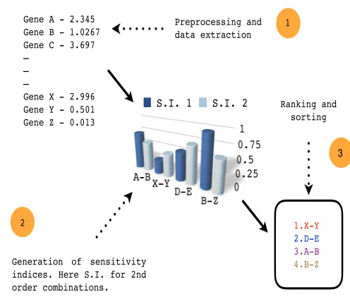
rank-Gene A - 2.345 Gene B - 1.0267 Gene C - 3.697 —

— —

Gene X - 2.996 Gene Y - 0.501 Gene Z - 0.013

Generation of sensitivity indices. Here S.I. for 2nd order combinations.

S.I. 1 S.I. 2

1.X-Y

2.D-E 3.A-B 4.B-Z Preprocessing and

data extraction

Ranking and sorting 1

2

3

Fig. 1Schematic view of the pipeline. Execution begins with preprocessing and extraction of data, followed by generation of sensitivity indices and culminating in ranking and sorting of the indices and the associated combinations. See steps 1., 2. and 3.

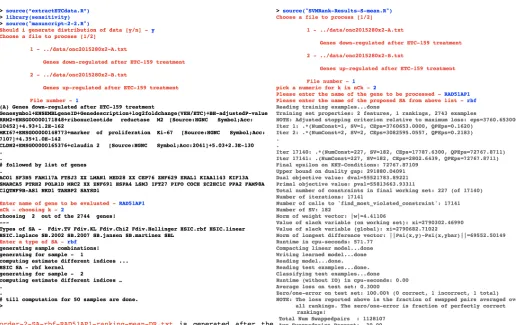
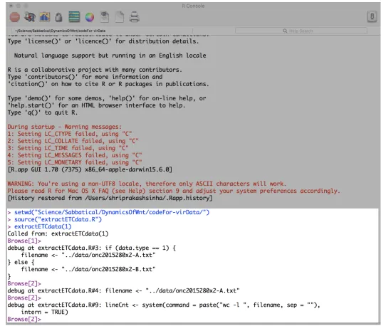
ing of the sensitivity indices. However, for a more professional-ized version, the pipeline can be divided into smaller independent modules. The schematic diagram of the pipeline is represented in figure 1. A snapshot of the code of execution of the full pipeline is shown in figure 2. Also, the code in R is presented and the coding is explained, where necessary. Note that explanation for the working of any particular package that has been used in the pipeline will not be provided. Instead, references will be provided for these packages or executable files.

2 Source and description of data

Data used in this research work was released in a publication by Madanet al.4. The ETC-1922159 was released in Singapore in July 2015 under the flagship of the Agency for Science, Tech-nology and Research (A*STAR) and Duke-National University of Singapore Graduate Medical School (Duke-NUS). Note that the ETC-1922159 data show numerical point measurements that is as4 _{quote - "List of differentially expressed genes identified at}

(3)

Fig. 2A snapshot of the code of execution of the full pipeline.

log₂

V EHg

ET Cg

(1)

3 Steps of execution via code elucidation

Fonts used for different constituents of the code -•variables in file and arguments initalics;•file names insans serif;•functions inbold;•R code is in verbatim.

3.1 Preprocessing of ETC-1922159 data

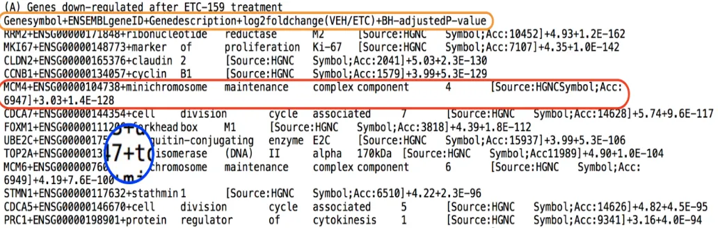
We begin with the first step of the search engine by processing the data that has been provided in Madanet al.4. Note that the data had to be manually preprocessed in order to store it in a de-sired format in a file (here a .txt file). Since the file contained a list of both down and up regulated genes, it was necessary to segregate them in two files. A snap shot of the manually pre-processed file is shown in figure 3. In this file, the down reg-ulated genes affected by ETC-1922159 have been stored. The

(4)

Fig. 3A snapshot of the manually processed file. In this file, the down regulated genes affected by ETC-1922159 have been stored. Orange boundary - contains the file header with different columns separated by a delimiter, here, "+" symbol.

3.2 Extraction of ETC-1922159 data

Once the data has been stored in the required format after manual preprocessing, the next step involves the extraction of data from these files and storage of the information in a requisite format. This is done using the fileextractETCdata.Rwhich contains the functionextractETCdata. We begin with the explanation of the code in a sequential manner below.

3.2.1 Description of extractETCdata.R

The function extractETCdata takes in the argument with the namedata.typethat is a numerical value. Here, if thedata type =1(2) then name of the file containing down(up) regulated genes is stored in thefilename. Theifcondition is used for as-signing the file name tofilenamewith the condition as argument

data.type==1(See lines 1-7 below).

1 extractETCdata <- function(data.type){

2 if(data.type == 1){

3 filename <- "../data/onc2015280x2-A.txt"

4 }else{

5 filename <- "../data/onc2015280x2-B.txt"

6 }

7

Next, the total number of lines needs to be known once the file to be worked on has been decided. This is required in order to know the number of entries in the file, which gives the list of genes. The processing begins with thesystemcommand which executes Unix utilities likewcor word count with an option to count linesl. We use the option ofinternto capture the output of the commandwc

in the output (see line 9 below). The output from the command is stored inlineCnt. This output is in the form of a string and the goal is to know the line count from this string. To proceed,

thestrsplitfunction is used in order to break up string inlineCnt

into the atomic elements. Further, since the output of thestrsplit

is in the form of a list, to simplify the data structure,unlist is used produce a vector of atomic elements with an argument str-split(lineCnt, " "). So here the output ofstrsplit(lineCnt, " ") goes as argument in the functionunlist. The output ofunlistwhich is a vector is stored inx(see line 10 below). Next, to extract the numerical value of the number of lines in the file, aforcommand is run, were the iteratoritakes in one element of vector in xat a time (see line 11 below) and tests if it is a numeric value. If a numeric value is found, theforloop breaks, else continues with the next element ofxin the iterator. So, for every value ofxini,

ifvalue inias numeric is not found to be true or is missing/not available, the iterator moves to the next element ofx. Else, if the value inias numeric is found to be true in theifcondition, then this value is assigned tonLinesand the execution breaks out of theforloop (see lines 11-14).

8 # find total number of lines in the file

9 lineCnt <- system(command=paste("wc -l ",

filename,sep=""),intern=TRUE)

10 x <- unlist(strsplit(lineCnt," "))

11 for(i in x){

12 if(is.na(as.numeric(i))){}

13 else{nLines <- as.numeric(i); break;}

14 }

15

(5)

informa-tion is contained in the block within thewhileloop, which starts from line 20. Thewhileruns till a condition is no longer true. Before that, the file needs to be openned for processing. This is done using thefilecommand which takes infilename as the ar-gument for variabledescriptionandrto read, as the argument for variableopen. This opens the connection for the file of interest and the connection to the file is stored in a variableconnecTion. We also set the variablecntto 0 as an iterator for thewhileloop that needs to execute as long as the conditioncnt≤nLinesas ar-gument to thewhileis met (see line 20). If the condition in line 20 is not met, the execution exits thewhileloop block.

Once inside the condition is satisfied, the counter is incre-mented by 1, stating that the first line is being read. This is indicated by updatedcnt value in line 21. Next, thecntth line is read from the file using the functionreadLineswhich take in as arguments the value inconnecTion and n(as 1 to read only one line). The output is thecntth line that is stored insentence. For processing purpose the sentence is concatenated with a return character. However, if thecntth_{line is the first line, then the loop}

just skips it and jumps to the next line in the file (see lines 16-24).

16 # extraction information from the file

17 connecTion <- file(description = filename,

open = "r")

18 cnt <- 0

19 #browser()

20 while(cnt <= nLines){

21 cnt <- cnt + 1

22 sentence <- readLines(con = connecTion,

n = 1)

23 cat(sentence,"\n")

24 if(cnt == 1){}

However, if thecntthline is the2ndone in the file, then we know that it contains the information on column names. This needs to be extracted from thesentencevariable in the second iteration of thewhileloop which extends from lines 25 to 59. Again, to explain the aspects of the code, we will break thiselse if(cnt= 2){...} block into parts. This block contains twoforloop blocks. The first block is used to retrieve the names of the columns that are delimited by a "+" sign (see lines 25-45). The second block is to create corresponding variable names that match with the retreived names followed by initialization (see lines 46-58).

Theelse ifblock begins with a few initializations. The cntth

sentence is split and stored in a simple format intempSentence. The length of the sentence in terms of the number of characters is stored in tempSentenceLength. The position of the delimiter "+" within the sentence is also stored using thewhichfunction. Finally, the names of the columns need to be stored in cnames

and an indexindx is used as a start position at a particular lo-cation in tempSentence for processing purpose. In the firstfor

loop, with the iteratoritaking on values of the position of the delimiter (stored indelimPlusPos) one at a time in every loop, a particluar piece of code is executed depending on the value of the index position inindx. In line 31, if the location of theindxis 1, i.e the starting character of the sentence, then the first name needs to be extracted that lies between position1 and position (i-1). Note at locationi, there is a "+" symbol. To execute this, the commandcapture.outputis used that converts the concate-nated elements of tempSentence[1:(i-1)] viacatcommand (see line 33). capture.outputcoverts the input argument in a string and stores the retreived name intempName. Next, this column name is stored incnamesin line 34. In case theindxis the po-sition which contains the last delimiter i.e.length(delimPlusPos) then the last and the penultimate column names need to be re-treived. The penultimate column name can be retreived from the characters between the penultimate delimiter and the last delim-iter, i.edelimPlusPos[indx-1]+1):(i-1)(see line 36). The last col-umn name can be retreived after the last delimiter and end of the sentence, i.edelimPlusPos[indx]+1):tempSentenceLength(see line 38). Finally, if the iterator neither points to the1st _{or the last} length(delimPlusPos) delimiter position, then the column name can be retrieved from characters lying between the position of the previous delimiter position and current delimiter position, i.e

(delimPlusPos[indx-1]+1):(i-1)(see line 41). Each of these are ranges that are encased in the vectortempSentenceand are con-catenated viacatand captured intempNameand later stored in

cnames. After the execution of the forloop ends, that is the it-erator ihas covered all the delimiter positions indelimPlusPos,

cnamescontains all the column names (see lines 31-45).

25 else if(cnt == 2){

26 tempSentence <- unlist(strsplit(

x = sentence, split = "+"))

27 tempSentenceLength <- length(tempSentence)

28 delimPlusPos <- which(tempSentence == "+")

29 cnames <- c()

30 indx <- 1

31 for(i in delimPlusPos){

32 if(indx == 1){

33 tempName <- capture.output(

cat(tempSentence[1:(i-1)],sep=""))

34 cnames <- c(cnames, tempName)

35 }else if(indx == length(delimPlusPos)){

36 tempName <- capture.output(cat(

tempSentence[(delimPlusPos[indx-1]+1):

(i-1)], sep=""))

tempSentence[(delimPlusPos[indx]+1):

(6)

40 }else{

(i-1)], sep=""))

43 }

44 indx <- indx + 1

45 }

Once the names of the column has been stored, the correspond-ing variables need to be created and initialized. This is done in the second block as described above. The secondforloop iter-ates through the list of column names. In each iteration of the

forloop, a condition is checked which tests whether a particu-lar pattern exists within the column name under consideration. If the condition is satisfied, as above, the corresponding variable is created and initialized. We use thegrepfunction to find the

patternin the column namei, asiiterates throughcnamesin the

forloop. If there is a match and the pattern exists in column namei, then the length of this match will not be equal to 0, like (length(grep(pattern = "sym",x= i)) != 0) on line 47. When this happens, the creation and initialization of a variable follows. In the above example,Genesymbolis created and initialized. Fi-nally, the block forelse ifis completed, if one is dealing with the

2nd_{line of the file (see lines 46-58).} 46 for(i in cnames){

47 if(length(grep(pattern = "sym",

x = i)) != 0){

48 Genesymbol <- c()

49 }else if(length(grep(pattern = "ID",

x = i)) != 0){

50 ENSEMBLgeneID <- c()

51 }else if(length(grep(pattern = "des",

x = i)) != 0){

52 Genedescription <- c()

53 }else if(length(grep(pattern = "fold",

x = i)) != 0){

54 logTwoFC <- c()

55 }else if(length(grep(pattern = "value",

x = i)) != 0){

56 BHadjustedPvalue <- c()

57 }

58 }

Next, for allcntth line of the file that is neither1st _or

2nd_{, the}

last part of theelseblock for the whileloop in line 20 is exe-cuted. This block is encoded in lines 59-82. Most of the code is similar to the preceeding block with a few changes. Line 60 contains the same command to store the sentence read atcntth

line of the file and line 61 is used to find the positions where the delimiter is positioned. In the next step, if there is an error in positioning of the delimiter due to manual preprocessing error, the command shows that correction needs to be done at linecnt. From lines 64 to 83, the coding is similar to the foregoing piece of code, except that if the indexindxis1, now, the name of the gene is stored inGenesymbol; if the indexindxislength(delimPlusPos) thenlog₂fold change values are stored inlogTwoFCfrom the left side of the delimiter and adjusted P-values are stored in BHad-justedPvaluefrom the right side of the delimiter; ifindxis 2, then ENSEMBLgeneID value is stored inENSEMBLgeneIDand finally, if

indxis 3, then Genedescription is stored inGenedescription. Lines starting with # are commented and used only for testing pur-pose and do not give any value (see lines 59-84). Note that as each line is read, information is stored usingrbindfunction that keeps attaching or binding the current value to the existing vec-tor in a variable. For example,Genesymbol<-rbind(Genesymbol,

tempName) will appendGenesymbolwith the currenttempName

thus increasing the size of the vector inGenesymbolby 1. This procedure gets repreated. Thus ends the storage of information regarding from the file in the variables.

59 }else{

60 tempSentence <- unlist(strsplit(

x = sentence, split = "+"))

61 delimPlusPos <- which(tempSentence == "+")

62 if(length(delimPlusPos) != 4){

cat("Correction needed at - ",cnt);

break

}

63 indx <- 1

64 for(i in delimPlusPos){

65 if(indx == 1){

tempSentence[1:(i-1)],sep=""))

67 Genesymbol <- rbind(Genesymbol, tempName)

68 }else if(indx == length(delimPlusPos)){

(i-1)], sep=""))

70 logTwoFC <- rbind(logTwoFC,

as.numeric(tempName))

71 # tempName <- capture.output(cat(

# tempSentence[(delimPlusPos[indx]+1):

# (tempSentenceLength-1)], sep=""))

tempSentence[delimPlusPos[indx]+(1:7)],

sep=""))

73 BHadjustedPvalue

(7)

74 }else if(indx == 2){

(i-1)], sep=""))

76 ENSEMBLgeneID <- rbind(ENSEMBLgeneID,

tempName)

77 }else if(indx == 3){

(i-1)], sep=""))

79 Genedescription

<-rbind(Genedescription, tempName)

80 }

81 indx <- indx + 1

82 }

83 }

84 }

Next, we close the open file using the commandclosewith an ar-gumentconnecTion. And finally, we combine the variable names in a data frame, a kind of data structure usingdata.frameand ar-gumentsGenesymbol,ENSEMBLgeneID,Genedescription,logTwoFC

andBHadjustedPvalue. The data frame is stored in the variable

oncETC. Finally, the return command returns this data frame as output using the functionreturnandoncETC(see lines 85-89).

85 close(connecTion)

86

87 oncETC <- data.frame(Genesymbol,

ENSEMBLgeneID, Genedescription,

logTwoFC, BHadjustedPvalue)

88 return(oncETC)

89 }

Note that the preprocessing and extraction of data can have dif-ferent flavours depending on the type of data and experiment one is dealing. However, the output of the extraction should be a data frame (a kind of variable in R) containing the extracted data that needs to be used in sensitivity analysis. This is explained next.

3.2.2 Exercise

As an exercise, the readers are encourged to build their own pre-processed file manually, from the data given in Madanet al.4and see if they can reproduce the results in the form of a data frame using the functionextractETCdata.

3.3 Computing the sensitivity indices

We move on to the next stage of the pipeline were the sensitivity indices need to be generated. Why we are generating these in-dices and how it helps in ranking up a set of factors and its com-binations involved in the pathway have been discussed in Sinha1

and Sinha2. Here we concentrate on the implementation of the pipeline and explanation of the code only. The code has been saved in the file namemanuscript-2-2.R and one of the author has been lazy enough not to change the name of the code. How-ever, it also points to the fact that the author is not concerned with the show of expertise in nomenclature of file names and nei-ther does he wish to earn a PhD in nomenclature of file names. Moving to the main topic, the code begins with the definitions of some functions and inclusion of packages from which specific function can be used during programming.

3.3.1 Description of manuscript-2-2.R

Here, thelibraryfunction is used to call the package "sensitivity" which has been implemented in R and goes as an argument into the functionlibrary. Details of the package can be found in Pu-jolet al.8. Next we define a function, using the functionfunction

and give this function a namenew.name. The function takes in as argument, a two dimensional matrixX.kis the number of genes under consideration out of a set of genes. Thenew.name imple-ments the g-function (a model) that is used to assign weights to each of the genes, with a random weight. For this,runiffunction is used. bis updated as each gene is considered one at a time in theforloop. At the end of the function, value inbis returned implicity. What happens is as the loop iterateslength(a) times, were the expression shows the number of genes the user has se-lected. Note that lenght ifais computed using the value of k. This function read within lines 3-10. Also,genSampleCombis a function which returns a two dimensional matrix with the a spe-cific number of columns defined inyCol. More about this function will be talked at a later stage. Here, definitions of the functions are provided (see lines 1-14).

1 library(sensitivity)

2 # Function definitions

3 new.fun <- function(X){

4 a <- runif(k)

5 b <- 1

6 for (j in 1:length(a)) {

7 _{b <- b * (abs(4 * X[, j] - 2) +}

a[j])/(1 + a[j])

8 }

9 b

10 }

11

12 genSampleComb <- function(yCol){

13 return(disty[,yCol])

14 }

15

(8)

point measurements, if they exist in the data under considera-tion. To query the user, the functionreadlineis employed. The user has to type in the option provided in the query for a partic-ular functionality to take affect. Here, the response to the query is stored in the variableDISTRIBUTION. Next, if the response in

DISTRIBUTIONis a yes, that is, the user typed in "y", then the ensuing block within theifcommand will get executed, else it will be skipped. Again, the block under consideration, defines a new functiongdfetppvwhich takes in argumentsnandyt, were

ncontains the number of points which a user might want to gen-erate for a distribution around a numerical point estimate. The measured numerical point estimates for each gene under consid-eration are assorted in a vectoryt. The length of ytshows the number of genes involved in the study of sensitivity analysis. As theforiterates through each gene, for the corresponding numer-ical point estimate for a partipular gene, a distribution around the point estimate is generated with the mean value beingyt[i]

(iis the iterator) and a standard deviation of0.₀₀₅_{. Along with}

the distribution a minor jitter or noise is added. Thus, the whole distribution is stored in a vector. Note that the output of the jit-terfunction is a vector and R stores vector in column format. Consequently, as theforloop iterates from one gene to another, the columns are bound together using a column binding func-tioncbind. Thus,randytkeeps on increasing column wise, till all genes have been covered. Once out of the loop, the row vec-torytis appended with the distribution matrixrandytusing row binding functionrbind. The output of the function is a two di-mensional matrix containing the point estimate in the first row and the corresponding distribution in the rows below (see lines 20-28).

16 # Generation of distributions

17 DISTRIBUTION <- readline("Should i generate

distribution of data [y/n] - ")

19 if(DISTRIBUTION == "y"){

20 gdfetppv <- function(n,yt){

21 randyt <- c()

22 lenyt <- length(yt)

23 for(i in 1:lenyt){

24 randyt <- cbind(randyt,

jitter(rnorm(n, mean = yt[i],

sd = 0.005), factor = 1))

25 }

26 yt <- rbind(yt, randyt)

27 return(yt)

28 }

29 }

After the functions have been defined, the main execution begins. The code starts with the extraction fo the data using the read-lineargument and provides an option to the used to choose file

that contains data regarding down regulated genes or up regu-lated genes. Once the respone is recorded, it is stored in the vari-ableDATATYPE. If the user enters a wrong number, then awhile

loop is run which asks to enter the right response. This feed-back continues till the user enters the right response (see lines 30-33). After the correct response is recorded, we use the func-tionextractETCdatato extract the information from the partic-ular file associated with the response inDATATYPE. This is done using the commandextractETCdata(DATATYPE) and the output of the function is stored inoncETCmain. We keep a copy of the stored information inoncETCmainand make a second copy in the subsequent line inoncETC(see line 34-35). This manuscript ex-plains the code for retrieving2nd

order combination, only so as to set a platform for many who would be reading the article. Note, before the use of the function i.e. instantiation of the function, the function needs to be defined and initialized. We defined the function and named it. After that an instance of the function is used to get a certain result. One instance isextractETCdata(1) and another instance isextractETCdata(2).

30 # Data extraction

31 DATATYPE <- readline("Choose a file to

process [1/2] \n

1 - ../data/onc2015280x2-A.txt \n

Genes down-regulated after ETC-159

treatment \n

2 - ../data/onc2015280x2-B.txt \n

Genes up-regulated after ETC-159

treatment \n

File number - ")

32 while(DATATYPE != "1" & DATATYPE != "2"){

DATATYPE <- readline("Type the kind of

data to be processed [1/2] - ")

33 }

34 oncETCmain <- extractETCdata(DATATYPE)

35 oncETC <- oncETCmain

Of interest is the column containing thelog₂fold change numer-ical point estimates that are stored in the variableoncETC. Since the information under this column is stored in the data frame, it needs to be converted into a matrix for further processing by sensitivity analysis package. For this,as.matrixfunction is used which takes in the object inx along with argumentsncolwhich asks for the number of columns into which the information needs to be divided andbyrowbeing false stating that the information will not be lined up row wise, but column wise. The result of the transformation is stored iny. Next, respective column ele-ments inyare allotted their gene names. This is acheived using

(9)

of number of rows and number of columns is recorded using the functiondimand the measurements are stored indim.y.dim.y[1]

contains the number of rows which implicitly defines the number of genes (stored in no.genes). The whole list of genes can be shown on the command prompt during the execution of the code viacat(rownames(y)) (see lines 35-40).

35 y <- as.matrix(x = oncETC$logTwoFC,

ncol = 1, byrow = FALSE)

36 rownames(y) <- oncETC$Genesymbol

37 factor.names <- oncETC$Genesymbol

38 dim.y <- dim(y)

39 no.genes <- dim.y[1]

40 cat(rownames(y))

Next, the user is asked which gene the user would like to inves-tigate and the response is stored ingeneName. Also, since the pipeline is about investigating combinations, we need to input the number of combinations we are interested in. For this, a similar query is asked and the value is stored in the variablek. Since it is in the character format, it needs to be converted into a numerical format and that is done usingas.numericfunction. Thecat func-tion helps in displaying messages to ease the user to understand what is happening while execution of the program. The combina-tions that can be generated fromkgenes, out of the total number of genesno.genesis computed usingcombn. This returns a two dimensional matrix togeneCombwhose number of columns rep-resent the total number of combinations, i.edim(geneComb[2]) (see lines 41-47).

41 geneName <- readline("\nEnter name of

gene to be evaluated - ")

42 # Regarding combinations

43 ANSWER <- readline("nCk - choosing k - ")

44 k = as.numeric(ANSWER)

45 cat("choosing ",k," out of the",

no.genes," genes!\n---\n")

46 geneComb <- combn(no.genes,k)

47 no.geneComb <- dim(geneComb)[2]

Next, initialization of the variables needs to be done for process-ing of the data. A series of list data structure is initialized and names are assigned to each new list as shown from lines 49 to 60. These are the variables where the sensitivity indicies will be stored. siNamescontains the names of the indicies which the search engine uses and the user can pick any one of them for computation. Line 63 prompts the user to enter the name of the sensitivity index, after looking at displayed list in the command on line 62. This name is stored in the variablevarName. Next, we search for the pattern (stored invarName) in some of the Sobol index names and if the user has chosen a sobol sensitivity index,

thenISSOBOLis assigned to a true value. This will be used and explained later on (see lines 49-66).

48 # some initializations

49 sensiFdiv.TV <- list()

50 sensiFdiv.KL <- list()

51 sensiFdiv.Chi2 <- list()

52 sensiFdiv.Hellinger <- list()

53 sensiHSIC.rbf <- list()

54 sensiHSIC.linear <- list()

55 sensiHSIC.laplace <- list()

56 SB.jansen <- list()

57 SB.2002 <- list()

58 SB.2007 <- list()

59 SB.martinez <- list()

60 SBL <- list()

61 siNames <- c("Fdiv.TV", "Fdiv.KL",

"Fdiv.Chi2", "Fdiv.Hellinger", "HSIC.rbf",

"HSIC.linear", "HSIC.laplace", "SB.2002",

"SB.2007", "SB.jansen", "SB.martinez", "SBL")

62 cat("Types of SA - ", siNames, "\n")

63 varName <- readline("Enter a type of SA - ")

64 ISSOBOL <- FALSE

65 if(length(grep(varName, "SB.2002"))!= 0 |

length(grep(varName, "SB.2007"))!= 0 |

length(grep(varName, "SB.jansen"))!= 0 |

length(grep(varName, "SB.martinez"))!= 0

| length(grep(varName, "SBL"))!= 0){

ISSOBOL <- TRUE

66 }

Regarding the generation of distribution of numerical point mea-surements, it is important to specify the number of samples. The user is usually given a choice as shown in line 67 (here com-mented). However, for exercise purpose, we set the value of num-ber of samples to ben=₁₀. Next, the function for generating distribution of size9per gene measurement is used and the out-put is converted into a data frame using the functiondata.frame. This data frame is then stored in variabledistyor distribution of y. We again save the number of samples as an extra using thedim

function, in a variableno.Samples(see lines 67-71).

67 # n <- as.numeric(readline("Enter number of

samples for distribution (odd numeric) - "))

68 n <- 9

69 disty <- data.frame(gdfetppv(n,t(y)))

70 no.Samples <- dim(disty)[1]

71 cat("generating sample combinations!\n")

(10)

here in the sense that we need to compute the indices for combi-nations of factors. The arguments forapplytake in a matrix, the indicator for a vector in a matrix over which a function will be applied. Here we see thatgeneCombis the matrix containing the combinations of genes;MARGIN with an indicator 2 means the columns ofgeneCombwill be worked upon by the function gen-SampleCombin the variableFUN. Thus the functionapplywill apply the functiongenSampleCombto the columns of the matrix

geneComb. The functiongenSampleCombin line 12, takes in a column of the matrixgeneComb and returns thek distributions that are stored in the matrixdisty. So, ifkis 2, then the number of rows ingeneCombwill be 2. These 2 elements associated with a particular column ingeneCombwill contain the gene numbers in a list of genes. During the application of theapplyfunction,yCol

stores a column ofgeneComband usesgenSampleCombto gen-eratedisty[,yCol], an_×k_{matrix, were}n_{is number of samples}

andk_{is the number of elements in combination. The procedure}

is applied to all columns ofgeneComb, for this. (see line 72).

72 distyN <- apply(X = geneComb, MARGIN = 2,

FUN = genSampleComb)

Next, the combinatorial distributions stored in distyN are pro-cessed to segregate the gene combinations that contain the par-ticular gene of interest defined by the user from a list of gene, ingeneName. List variables are defined and to find combinations containinggeneName, aforloop is executed were the iterator it-erates through the total number ofCn

k combinations. For each

of the combination contained innames(distyN[i]), ifgeneNameis found to be existing, then the distribution containinggeneName

and another gene indistyN[i]is stored inx.S, a list. For every such identification, a counter cnt is incremented. Finally, after all combinations have been found which containgeneName, the final cnt _{is assigned to number of selected gene combinations} no.slgeneComb(see lines 73-85).

73 # Sample with replicates

74 x.S <- list()

75 x.Sfh <- list()

76 x.Ssh <- list()

78 cnt <- 0

79 for(i in 1:no.geneComb){

80 if(geneName %in% names(distyN[[i]])){

81 cnt <- cnt + 1

82 x.S[[cnt]] <- distyN[[i]]

83 }

84 }

85 no.slgeneComb <- cnt

Usually a user will be asked about the total number of iterations for which the sensitivity indicies will be generated. This is done

to get an average sensitivity index score which is then used for ranking of the combinations. For demonstration purpose, we set the iteration number toitrNo=50. Theforloops the iterator

tr _for₅₀ _{iterations. Every iteration, the number of interation}

is displayed at the start of theforloop. The samples need to be shuffled every time in order to have variation so that the mean of the sensitivity indices can be generated. This can be done by using the functionsamplewhich take a range of values from1

tono.Samples and the size of the sample is set to no.Samples. The shuffled samples are stored insample.index.idx.fhandidx.sh

are used to divide the sample into two halves, in case one is us-ing Sobol method for generatus-ing sensitivity indicies. Next, if the method used is Sobol or a variant of the same, as indicated by

SSOBOL_{, then shuffling of the samples in combination happens.}

This shuffling is done in lines 99-100, for all combinations, i.ej

from 1 tono.slgeneComb. For, non Sobol based methods, the shuf-fling is simple as shown in line 104.

86 # itrNo <- as.numeric(readline("Number

of iterations for averaged ranking - "))

87 itrNo <- 50

88 hmean <- list()

89 for(itr in 1:itrNo){

90 # disty <- data.frame(gdfetppv(n,yt))

91 # distyN can be replaced with x.S also

92 cat("generating for sample - ", itr, "\n")

93 sample.index <- sample(x = 1:no.Samples,

size = no.Samples)

94 idx.fh <- sample.index[1:(no.Samples/2)]

95 idx.sh <- sample.index[((no.Samples/2)+1)

:no.Samples]

96 # Shuffle the samples

97 if(ISSOBOL){

98 for(j in 1:no.slgeneComb){

99 x.Sfh[[j]] <- x.S[[j]][idx.fh,]

100 x.Ssh[[j]] <- x.S[[j]][idx.sh,]

101 }

102 }else{

103 for(j in 1:no.slgeneComb){

104 x.S[[j]] <- x.S[[j]][sample.index,]

105 }

106 }

(11)

needs to be taken into account and necessary method to be initi-ated to generate the indicies. One of the approach would be to usegrepfunction which searches for a pattern invarName. If the pattern exists, then the length of the finding would not be zero. When this condition holds, then a particular index associated with the pattern is intiated. So, if "TV" is the pattern and it found to be in thevarName, then f-divergence method9with a Total variation distance|t₋₁_|_{needs to be initiated. The short explanation on}

the theoretical principles of density and variance based methods has been explained in3_{. Here we concentrate on the flow of the}

code. In line 109, we define and initialize a new variableFdivTV. After some displays on the screen,lapplyis used onx.S.lapply

returns a list of the same length asx.S, each element of which is the result of applying functionsensiFdivto the corresponding element ofx.S. Additionally, since the sensitivity method uses a model function, we use extra arguments in thelapplyfunction, likemodel=new.fun;nboot= 0 andconf = 0.95. Thisnew.fun

has earlier been defined in the beginning of the code. So,lapply

generates sensitivity indices for each of the matricies containing a specific gene combination using thenew.funviasensiFdiv. The result is stored in a variableh. Since we know thatlapplywill generate sensitivity indices for each of the matrices inx.S, thus each combination has an associated sensitivity that is stored in

h[[p]]$S$original. We bind this to the variableFdivTV (see lines 108-113).

Next, since theforloop in line 89 works for many iterations, we need to store the sensitivity index computed in this iteration in a certain variable. This is done insensiFdiv.TV[[itr]], definition of which was done in line 49. Also, if this is the first iteration, then we define the file name based on the data that is being used and the iteration (see lines 115-117).

107 # itr <- 1

108 if(length(grep("TV",varName))!= 0){

109 FdivTV <- c()

110 cat("computing estimate different

indices ...\n")

111 cat("Fdiv SA - TV\n")

112 h <- lapply(x.S, sensiFdiv,

model = new.fun, fdiv = "TV",

nboot = 0, conf = 0.95)

113 for(p in 1:no.slgeneComb){

FdivTV <- cbind(FdivTV,

h[[p]]$S$original)

}

114 sensiFdiv.TV[[itr]] <- FdivTV

115 if(DATATYPE == "1" & itr == 1){

filename <- paste("order-",k,"-",

geneName,

"-DR-A-ETC-T-fdiv-tv-mean.Rdata",

sep = "")

116 }else if(DATATYPE == "2" & itr == 1){

filename <- paste("order-",k,"-",

geneName,

"-UR-A-ETC-T-fdiv-tv-mean.Rdata",

sep = "")

117 }

The next series of conditions deals with the different methods in a similar manner as explained for lines 108-117. Lines 118-130 talk about f-divergence method9 _{with a Kullback-Leibler divergence}

−loge(t)_.

118 }else if(length(grep("KL",varName))

!= 0){

119 FdivKL <- c()

indices ...\n")

121 cat("Fdiv SA - KL\n")

model = new.fun, fdiv = "KL",

nboot = 0, conf = 0.95)

124 FdivKL <- cbind(FdivKL,

h[[p]]$S$original)

125 }

125 sensiFdiv.KL[[itr]] <- FdivKL

126 if(DATATYPE == "1" & itr == 1){

127 filename <- paste("order-",k,"-",

geneName,

"-DR-A-ETC-T-fdiv-kl-mean.Rdata",

sep = "")

geneName,

"-UR-A-ETC-T-fdiv-kl-mean.Rdata",

sep = "")

130 }

Lines 131-144 talk about f-divergence method9 _{with a}χ2

dis-tancet2−1.

131 }else if(length(grep("Chi2",varName))

!= 0){

132 FdivChi2 <- c()

indices ...\n")

134 cat("Fdiv SA - Chi2\n")

model = new.fun, fdiv = "Chi2",

(12)

137 FdivChi2 <- cbind(FdivChi2,

h[[p]]$S$original)

138 }

139 sensiFdiv.Chi2[[itr]] <- FdivChi2

140 if(DATATYPE == "1" & itr == 1){

geneName,

"-DR-A-ETC-T-fdiv-chi2-mean.Rdata",

sep = "")

geneName,

"-UR-A-ETC-T-fdiv-chi2-mean.Rdata",

sep = "")

144 }

Lines 145-158 talk about f-divergence method9with a Hellinger distance(p

(t₎₋₁₎2_.

145 }else if(length(grep("Hellinger",varName))

!= 0){

146 FdivHellinger <- c()

indices ...\n")

148 cat("Fdiv SA - Hellinger\n")

model = new.fun, fdiv = "Hellinger",

nboot = 0, conf = 0.95)

151 FdivHellinger <- cbind(FdivHellinger,

h[[p]]$S$original)

152 }

153 sensiFdiv.Hellinger[[itr]]

<- FdivHellinger

154 if(DATATYPE == "1" & itr == 1){

geneName,

"-DR-A-ETC-T-fdiv-hellinger-mean.Rdata",

sep = "")

geneName,

"-UR-A-ETC-T-fdiv-hellinger-mean.Rdata",

sep = "")

158 }

Da Veiga10recently proposed a new set of dependence measures using kernel methods. These also, have been implemented in Pu-jolet al.8. The following contains variants of different kernels involved in computing the sensitvity indices. Lines 159-172 show

similar execution code as above with changes insome of the ar-guments in thelapply function. Here, the "rbf" or radial basis function is used withinsensiHSIC.

159 }else if(length(grep("rbf",varName))

!= 0){

160 HSICrbf <- c()

indices ...\n")

162 cat("HSIC SA - rbf kernel\n")

163 h <- lapply(x.S, sensiHSIC,

model = new.fun, kernelX = "rbf",

paramX = NA, kernelY = "rbf",

paramY = NA, conf = 0.95)

165 HSICrbf <- cbind(HSICrbf,

h[[p]]$S$original)

166 }

167 sensiHSIC.rbf[[itr]] <- HSICrbf

168 if(DATATYPE == "1" & itr == 1){

geneName,

"-DR-A-ETC-T-hsic-rbf-mean.Rdata",

sep = "")

geneName,

"-UR-A-ETC-T-hsic-rbf-mean.Rdata",

sep = "")

172 }

Lines 173-186 show similar execution code as above with changes insome of the arguments in thelapplyfunction. Here, the linear function is used.

173 }else if(length(grep("linear",varName))

!= 0){

174 HSIClinear <- c()

indices ...\n")

176 cat("HSIC SA - linear kernel\n")

model = new.fun, kernelX = "linear",

paramX = NA, kernelY = "linear",

179 HSIClinear <- cbind(HSIClinear,

h[[p]]$S$original)

180 }

181 sensiHSIC.linear[[itr]] <- HSIClinear

(13)

geneName,

"-DR-A-ETC-T-hsic-linear-mean.Rdata",

sep = "")

geneName,

"-UR-A-ETC-T-hsic-linear-mean.Rdata",

sep = "")

186 }

Lines 187-200 show similar execution code as above with changes insome of the arguments in thelapplyfunction. Here, the laplace function is used.

187 }else if(length(grep("laplace",varName))

!= 0){

188 HSIClaplace <- c()

indices ...\n")

190 cat("HSIC SA - laplace kernel\n")

model = new.fun, kernelX = "laplace",

paramX = NA, kernelY = "laplace",

193 HSIClaplace <- cbind(HSIClaplace,

h[[p]]$S$original)

194 }

195 sensiHSIC.laplace[[itr]] <- HSIClaplace

196 if(DATATYPE == "1" & itr == 1){

geneName,

"-DR-A-ETC-T-hsic-laplace-mean.Rdata",

sep = "")

geneName,

"-UR-A-ETC-T-hsic-laplace-mean.Rdata",

sep = "")

200 }

Finally, we come to the section, were variants of the Sobol func-tion have been encoded. It is here that the use of divided samples

X.SfhandX.Sshcomes to play. We do not use thelapplyfunction. Instead, the Sobol’11variants are enconded using name specific function (see below). Lines 201-214 show similar execution code as above, but usingsoboljansen.

201 }else if(length(grep("jansen",varName))

!= 0){

202 SBLjansen <- c()

indices ...\n")

204 cat("Sobol Jansen SA\n")

206 h <- soboljansen(model = new.fun,

X1 = t(x.Sfh[[p]]),

X2 = t(x.Ssh[[p]]), conf = 0.95)

207 SBLjansen <- cbind(SBLjansen,

c(h$S$original, h$T$original))

208 }

209 SB.jansen[[itr]] <- SBLjansen

210 if(DATATYPE == "1" & itr == 1){

geneName,

"-DR-A-ETC-T-sb-jansen-mean.Rdata",

sep = "")

geneName,

"-UR-A-ETC-T-sb-jansen-mean.Rdata",

sep = "")

214 }

Lines 215-228 show similar execution code as above, but using

sobol2002.

215 }else if(length(grep("2002",varName))

!= 0){

216 SBL2002 <- c()

indices ...\n")

218 cat("Sobol 2002 SA\n")

220 h <- sobol2002(model = new.fun,

X1 = t(x.Sfh[[p]]),

X2 = t(x.Ssh[[p]]), conf = 0.95)

221 SBL2002 <- cbind(SBL2002,

222 }

223 SB.2002[[itr]] <- SBL2002

224 if(DATATYPE == "1" & itr == 1){

geneName,

"-DR-A-ETC-T-sb-2002-mean.Rdata",

sep = "")

geneName,

"-UR-A-ETC-T-sb-2002-mean.Rdata",

(14)

228 }

sobol2007.

!= 0){

230 SBL2007 <- c()

indices ...\n")

232 cat("Sobol 2007 SA\n")

234 h <- sobol2007(model = new.fun,

X1 = t(x.Sfh[[p]]),

X2 = t(x.Ssh[[p]]), conf = 0.95)

235 SBL2007 <- cbind(SBL2007,

236 }

237 SB.2007[[itr]] <- SBL2007

238 if(DATATYPE == "1" & itr == 1){

geneName,

sep = "")

geneName,

sep = "")

242 }

sobolmartinez.

243 }else if(length(grep("martinez",varName))

!= 0){

244 SBLmartinez <- c()

indices ...\n")

246 cat("Sobol Martinez SA\n")

248 h <- sobolmartinez(model = new.fun,

X1 = t(x.Sfh[[p]]),

X2 = t(x.Ssh[[p]]), conf = 0.95)

249 SBLmartinez <- cbind(SBLmartinez,

250 }

251 SB.martinez[[itr]] <- SBLmartinez

252 if(DATATYPE == "1" & itr == 1){

geneName,

"-DR-A-ETC-T-sb-martinez-mean.Rdata",

sep = "")

geneName,

"-UR-A-ETC-T-sb-martinez-mean.Rdata",

sep = "")

256 }

sobol.

257 }else if(length(grep("SBL",varName))

!= 0){

258 sbl <- c()

indices ...\n")

260 cat("SBL SA\n")

262 h <- sobol(model = new.fun,

X1 = t(x.Sfh[[p]]),

X2 = t(x.Ssh[[p]]), order = 1,

conf = 0.95)

263 sbl <- cbind(SBL, c(h$S$original,

h$T$original))

264 }

265 SBL[[itr]] <- sbl

266 if(DATATYPE == "1" & itr == 1){

geneName,

"-DR-A-ETC-T-sbl-mean.Rdata",

sep = "")

geneName,

"-UR-A-ETC-T-sbl-mean.Rdata",

sep = "")

270 }

271 }

272 }

Once the indices have been generated, they need to be stored in a file for further processing. The following set of lines help in saving the work, were the functionsave is used and variables

no.slgeneComb, x.Sand the respective sensitivity indices related tovarNameis stored in thefilename.

273 if(length(grep("TV",varName))!= 0){

274 save(no.slgeneComb, x.S,

sensiFdiv.TV, file = filename)

(15)

!= 0){

sensiFdiv.KL, file = filename)

277 }else if(length(grep("Chi2",varName))

!= 0){

sensiFdiv.Chi2, file = filename)

277 }else if(length(grep("Hellinger",varName))

!= 0){

sensiFdiv.Hellinger, file = filename)

279 }else if(length(grep("rbf",varName))

!= 0){

sensiHSIC.rbf, file = filename)

281 }else if(length(grep("linear",varName))

!= 0){

sensiHSIC.linear, file = filename)

283 }else if(length(grep("laplace",varName))

!= 0){

sensiHSIC.laplace, file = filename)

285 }else if(length(grep("jansen",varName))

!= 0){

SB.jansen, file = filename)

!= 0){

SB.2002, file = filename)

!= 0){

SB.2007, file = filename)

292 }else if(length(grep("martinez",varName))

!= 0){

SB.martinez, file = filename)

294 }else if(length(grep("SBL",varName))

!= 0){

SBL, file = filename)

296 }

This ends the coding part of estimating sensitvity indices. Once the indices are ready they can be used in various ways for evalua-tion of the combinaevalua-tions. Here, we use one of the ways to ranking these scores. However, not that there is no one definite rule to say that one has to rank in this way only. It depends on the research

to decide what method one is employing for ranking. We use the

SV MRnk _{algorithm by Joachims}12_{. Though complex in nature,}

it does a fair job in ranking the scores. The use of a machine learning approach is also made available to see how the learning algorithms play critical role in revealing unknown/untested com-binatorial hypotheses. Other reasons of using these will be stated later on.

3.3.2 Exercise

At this stage, it would be great to see how the two codes on ex-tracting data and generating indices works out. The readers are requested to generate the different types of indices based on their choice and see what comparisons can be made using the different indices. Also try the following exercies

-1. Generate HSIC rbf indices for 2nd

order combinations for downregulated AXIN2. What does the combination of AXIN2 with another factor that has lowest score mean?

2. Generate FDiv KL indices for 2nd order combinations for downregulated MYC. What does the combination of MYC with another factor that has highest score mean?

3. Generate HSIC laplace indices for2nd _{order combinations}

for downregulated NKD1. What does the combination of NKD1 with another factor that has score in the middle mean?

4. Generate FDiv TV indices for 2nd order combinations for downregulated CDAN1. What does the combination of CDAN1 with another factor that has score at 100 position in ascending order mean?

5. Generate Sobol indices for 2nd

order combinations for downregulated MINA. How many kinds of indices can you generate? Compare them for a particular combination!

6. Generate Sobol jansen indices for2nd order combinations for downregulated MINA. How many kinds of indices can you generate? Compare them for two different combina-tions!

7. Generate Sobol martinez indices for2nd

order combinations for downregulated MINA. How many kinds of indices can you generate? Compare them for 20 different combinations!

8. Generate Sobol 2002 and 2007 indices for2ndorder com-binations for downregulated MINA. How many kinds of in-dices can you generate? Compare Sobol 2002 vs Sobol 2007

(16)

3.4 Ranking

This part of the code is the last in the pipeline that works on the generated sensitivity indices. It ranks the sensitivity indices using a machine learning algorithm. We go through this part of the code and will then come back to why’s and why not’s. Lines 1-16 are basic data processing techniques and some formalities that need to be done befor we begin on the ranking part. So, by now, it should be expected the reader is able to work through the line and understand what is happening if a following line is being executed, at least, theoretically.

1 DATATYPE <- readline("Choose a file

to process [1/2] \n

2 1 - ../data/onc2015280x2-A.txt \n

3 Genes down-regulated after ETC-159

treatment \n

4 2 - ../data/onc2015280x2-B.txt \n

5 Genes up-regulated after ETC-159

treatment \n

6 File number - ")

7 while(DATATYPE != "1" & DATATYPE != "2"){

8 DATATYPE <- readline("Type the kind of

data to be processed - ")

9 }

10

11 CHOOSE <- as.numeric(readline("pick a

numeric for k in nCk - "))

12 k <- as.numeric(CHOOSE)

13

14 geneName <- readline("Please enter the

name of the gene to be processed - ")

15 siNames <- c("Fdiv.TV", "Fdiv.KL",

"Fdiv.Chi2", "Fdiv.Hellinger", "HSIC.rbf",

"HSIC.linear", "HSIC.laplace", "SB.2002",

"SB.2007", "SB.jansen", "SB.martinez",

"SBL")

16 sa.name <- readline("Please enter the

name of the proposed SA from above

list - ")

We stored the sensitivity indices in different files. These files need to be accessed in order for the procedure of ranking to be initi-ated. The following lines help retrieve the file names which can then be loaded into the R workspace from where it can be ac-cessed easily. To retrieve the file name, the functionpasteis em-ployed. Readers are encouraged to find how thepastefunction works. After the file name is constructed, the contents of the file are loaded using theloadfunction, followed by the assignment of stored data into a variableh. Lines 17-113 show the code for various kinds of indicies that a user can access, after usingpaste

andload.

17 if(length(grep(sa.name,"Fdiv.TV"))

!= 0){

18 if(DATATYPE == "1"){

geneName,

"-DR-A-ETC-T-fdiv-tv-mean.Rdata",

sep = "")

20 }else{

geneName,

"-UR-A-ETC-T-fdiv-tv-mean.Rdata",

sep = "")

22 }

23 load(filename)

24 h <- sensiFdiv.TV

25 }else if(length(grep(sa.name,"Fdiv.KL"))

!= 0){

geneName,

"-DR-A-ETC-T-fdiv-kl-mean.Rdata",

sep = "")

28 }else{

geneName,

"-UR-A-ETC-T-fdiv-kl-mean.Rdata",

sep = "")

30 }

31 load(filename)

32 h <- sensiFdiv.KL

33 }else if(length(grep(sa.name,"Fdiv.Chi2"))

!= 0){

geneName,

"-DR-A-ETC-T-fdiv-chi2-mean.Rdata",

sep = "")

36 }else{

geneName,

"-UR-A-ETC-T-fdiv-chi2-mean.Rdata",

sep = "")

38 }

39 load(filename)

40 h <- sensiFdiv.Chi2

41 }else if(length(grep(sa.name,"Fdiv.Hellinger"))

!= 0){

(17)

"-DR-A-ETC-T-fdiv-hellinger-mean.Rdata",

sep = "")

44 }else{

geneName,

"-UR-A-ETC-T-fdiv-hellinger-mean.Rdata",

sep = "")

46 }

47 load(filename)

48 h <- sensiFdiv.Hellinger

49 }else if(length(grep(sa.name,"HSIC.rbf"))

!=0){

geneName,

"-DR-A-ETC-T-hsic-rbf-mean.Rdata",

sep = "")

52 }else{

geneName,

"-UR-A-ETC-T-hsic-rbf-mean.Rdata",

sep = "")

54 }

55 load(filename)

56 h <- sensiHSIC.rbf

57 }else if(length(grep(sa.name,"HSIC.linear"))

!= 0){

geneName,

"-DR-A-ETC-T-hsic-linear-mean.Rdata",

sep = "")

60 }else{

geneName,

"-UR-A-ETC-T-hsic-linear-mean.Rdata",

sep = "")

62 }

63 load(filename)

64 h <- sensiHSIC.linear

65 }else if(length(grep(sa.name,"HSIC.laplace"))

!= 0){

geneName,

"-DR-A-ETC-T-hsic-laplace-mean.Rdata",

sep = "")

68 }else{

geneName,

"-UR-A-ETC-T-hsic-laplace-mean.Rdata",

sep = "")

70 }

71 load(filename)

72 h <- sensiHSIC.laplace

73 }else if(length(grep(sa.name,"SB.2002"))

!= 0){

geneName,

sep = "")

76 }else{

geneName,

sep = "")

78 }

79 load(filename)

80 h <- SB.2002

81 }else if(length(grep(sa.name,"SB.2007"))

!= 0){

geneName,

sep = "")

84 }else{

geneName,

sep = "")

86 }

87 load(filename)

88 h <- SB.2007

89 }else if(length(grep(sa.name,"SB.jansen"))

!= 0){

geneName,

"-DR-A-ETC-T-sb-jansen-mean.Rdata",

sep = "")

92 }else{

geneName,

"-UR-A-ETC-T-sb-jansen-mean.Rdata",

sep = "")

94 }

95 load(filename)

(18)

97 }else if(length(grep(sa.name,"SB.martinez"))

!= 0){

geneName,

"-DR-A-ETC-T-sb-martinez-mean.Rdata",

sep = "")

100 }else{

geneName,

"-UR-A-ETC-T-sb-martinez-mean.Rdata",

sep = "")

102 }

103 load(filename)

104 h <- SB.martinez

105 }else if(length(grep(sa.name,"SBL"))

!= 0){

geneName,

"-DR-A-ETC-T-sbl-mean.Rdata",

sep = "")

108 }else{

geneName,

"-UR-A-ETC-T-sbl-mean.Rdata",

sep = "")

110 }

111 load(filename)

112 h <- SBL

113 }

Once the indicies that have to be worked on have been put in

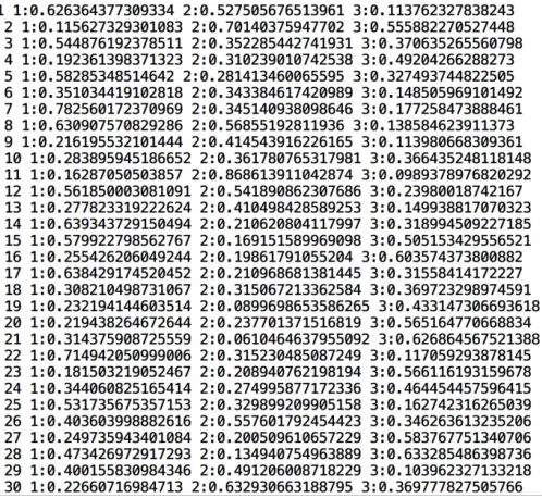
h, the indicies need to be averaged. For demonstration purpose, we average only 2 iterations and see how things turn out. How-ever, we need to understand how the data is stored inh. Fig-ure 4 shows a screen shot of how element ofh looks. h[[25]]

is the25th element and is a matrix of size 2×2743. 2is the number of elements in a combination under consideration and

2743are the total number of distinct2ndorder combinations. We exploit this view ofh to compute the means of for all ele-ments of a combination and over all distinct combinations. This is done in theforloops below in whichpiterates over elements of combination anditriterates over the total number of iterations. Thush[[itr]][p,]between the two nestedforloops considers the

pth row of itrth matrix in h. Then, r binds all the h[[1]][p,],

h[[2]][p,], ...,h[[itrNo]][p,], usingrbind. After exiting the inner loop, we use theapplyfunction tormatrix over the columns (i.e the distinct combinations) with a functionmean. Thus we get a vector of mean values of sensitivity index for each distinct

com-bination over all iterations, for thepth element. This process is again repeated for the nextpvalue. Finally, the vector of means are stacked inSAmean. Lines 114-124 show this coding below.

114 # Use this for averaged ranking

115 # itrNo <- 50

116 itrNo <- 2

117 SAmean <- c()

118 for(p in 1:k){

119 r <- c()

120 for(itr in 1:itrNo){

121 r <- rbind(h[[itr]][p,])

122 }

123 SAmean <- rbind(SAmean, apply(X = r,

MARGIN = 2, mean))

124 }

Next, we format the data in the form that is suitable for the

SV Mr nk_{machine. The output of the next block of code can be}

depicted in figure 5. Note that it is a screen shot for how the data is saved for a3r d

order combination. i invite readers to decode the following block by themselves as an exercise.

125 # y <- SA

126 y <- SAmean

127 data <- c()

128 for(i in 1:no.slgeneComb){

129 z <- c()

130 z <- cbind(z,i)

131 for(j in 1:k){

132 z <- cbind(z,

paste(j,":",y[j,i],sep=""))

133 }

134 z <- cbind(z,"\n")

135 data <- rbind(data,z)

136 }

Next the file names for traning, testing, model and predition are built using paste (see lines 137-140). And finally, data is concate-nated to the training and the testing files (see lines 141-142).

137 trnfl <- paste("svr-trn-order-",k,

"-",geneName,".txt", sep = "")

138 tstfl <- paste("svr-tst-order-",k,

139 mdlfl <- paste("svr-mdl-order-",k,

140 predfl <- paste("svr-pred-order-",k,

141 cat(t(data),file=trnfl)