Cryptanalysis on Full Grain-128a, Grain-128, and Grain-v1
Yosuke Todo1, Takanori Isobe2, Willi Meier3,
Kazumaro Aoki1, and Bin Zhang4,5
1 NTT Secure Platform Laboratories, Tokyo 180-8585, Japan 2
University of Hyogo, Hyogo 650-0047, Japan 3 FHNW, Windisch, Switzerland 4
TCA Laboratory, SKLCS, Institute of Software, Chinese Academy of Sciences, Beijing, China 5 State Key Laboratory of Cryptology, P.O.Box 5159, Beijing 100878, China
Abstract. A fast correlation attack (FCA) is a well-known cryptanalysis technique for LFSR-based stream ciphers. The correlation between the initial state of an LFSR and corresponding key stream is exploited, and the goal is to recover the initial state of the LFSR. In this paper, we revisit the FCA from a new point of view based on a finite field, and it brings a new property for the FCA when there are multiple linear approximations. Moreover, we propose a novel algorithm based on the new property, which enables us to reduce both time and data complexities. We finally apply this technique to the Grain family, which is a well-analyzed class of stream ciphers. There are three stream ciphers, Grain-128a, Grain-128, and Grain-v1 in the Grain family. As a result, we break them all, and especially for Grain-128a, the cryptanalysis on its full version is reported for the first time. Note that our attack is applied to the stream cipher mode of Grain-128a, and strong assumption is required to attack its authentication mode. Since ISO/IEC 29167-13 standardizes only authentication mode, our attack does not affect the practical use of the ISO/IEC standard.
Keywords: Fast correlation attack, Stream cipher, LFSR, Finite field, Multiple linear ap-proximations, Grain-128a, Grain-128, Grain-v1
1
Introduction
Stream ciphers are a class of symmetric-key cryptosystems. They commonly generate a key stream of arbitrary length from a secret key and initialization vector (iv), and a plaintext is encrypted by XORing with the key stream. Many stream ciphers consist of an initialization and key-stream gener-ator. The secret key and iv are well mixed in the initialization, where a key stream is never output, and the mixed internal state is denoted as the initial state in this paper. After the initialization, the key-stream generator outputs the key stream while updating the internal state. The initialization of stream ciphers generally requires much processing time, but the key-stream generator is very efficient.
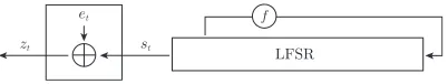
LFSRs are often used in the design of stream ciphers, where the update function consists of one or more LFSRs and non-linear functions. Without loss of generality, the key-stream generator of LFSR-based stream ciphers can be represented as Fig. 1, where the binary noiseet is generated by the non-linear function. LFSR-based stream ciphers share the feasibility to guarantee a long period in the key stream.
LFSR et
st
zt
f
A (fast) correlation attack is an important attack against LFSR-based stream ciphers. The initial idea was introduced by Siegenthaler [Sie84], and it exploits the bias ofet. We guess the initial state
s(0) = (s0, s1, . . . , s
n−1), computest for t =n, n+ 1, . . . , N −1, and XOR st with corresponding
zt. If we guess the correct initial state, highly biasedetis acquired. Otherwise, we assume that the XOR behaves at random. When we collect anN-bit key stream and the size of the LFSR isn, the simple algorithm requires a time complexity ofN2n.
Following up the correlation attack, many algorithms have been proposed to avoid the exhaustive search of the initial state, and they are called as “fast correlation attack.” The seminal work was proposed by Meier and Staffelbach [MS89], where the noiseetis efficiently removed fromztby using parity-check equations, and st is recovered. Several improvements of the original fast correlation attack have been proposed [ZYR90,MG90,CS91,JJ99b,JJ99a,CT00], but they have limitations such as the number of taps in the LFSR is significantly small or the bias of the noise is significantly high. Therefore, their applications are limited to experimental ciphers, and they have not been applied to modern concrete stream ciphers.
Another approach of the fast correlation attack is the so-called one-pass algorithm [CJS00,MFI01], and it has been successfully applied to modern concrete stream ciphers [BGM06,LLP08,ZXM15]. Similarly to the original correlation attack, we guess the initial state and recover the correct one by using parity-check equations. To avoid exhaustive search over the initial state, several methods have been proposed to decrease the number of secret bits in the initial state involved by parity-check equations [CJM02,ZF06]. In the most successful method, the number of involved secret bits decreases by XORing two different parity-check equations. Letet=hs(0), ati ⊕ztbe the parity-check equation, where hs(0), a
tidenotes an inner product betweens(0) and at, and we assume that et is highly biased. Without loss of generality, we first detect a set of pairs (j1, j2) such that the first`bits inaj1⊕aj2 are 0, where such a set of pairs is efficiently detected from the birthday paradox. Then,
hs(0), a
j1⊕aj2i ⊕zj1⊕zj2 is also highly biased, and the number of involved secret bits decreases from nton−`. Later, this method is generalized by the generalized birthday problem [Wag02]. Moreover, an efficient algorithm was proposed to accelerate the one-pass algorithm [CJM02]. They showed that the guess and evaluation procedure can be regarded as a Walsh-Hadamard transform, and the fast Walsh-Hadamard transform (FWHT) can be applied to accelerate the one-pass algorithm. While the naive algorithm for the correlation attack requires N2n, the FWHT enables us to evaluate it with the time complexity ofN+n2n. When the number of involved bits decreases fromnton−`, the time complexity also decreases to N + (n−`)2n−`. The drawback of the one-pass algorithm with the birthday paradox is the increase of the noise. Letpbe the probability thatet= 1, and the correlation denoted by c is defined as c = 1−2p. If we use the XOR of parity-check equations to reduce the number of involved secret bits, the correlation of the modified equations drops toc2. The
increase of the noise causes the increase of the data complexity.
Revisiting Fast Correlation Attack. In this paper, we revisit the fast correlation attack. We first
review the structure of parity-check equations from a new point of view based on a finite field, and the new viewpoint brings a new property for the fast correlation attack. A multiplication between
n×nmatrices and ann-bit fixed vector is generally used to construct parity-check equations. Our important observation is to show that this multiplication is “commutative” via the finite field, and it brings the new property for the fast correlation attack.
We first review the traditional wrong-key hypothesis, i.e., we observe correlation 0 when incorrect initial state is guessed. The new property implies that we need to reconsider the wrong-key hypothesis more carefully. Specifically, assuming that there are multiple high-biased linear masks, the traditional wrong-key hypothesis does not hold. We then show a modified wrong-key hypothesis.
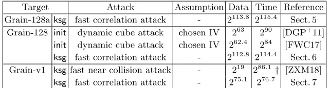
Table 1.Summary of results, where the key-stream generator and initialization are denoted asksgandinit, respectively.
Target Attack Assumption Data Time Reference Grain-128aksg fast correlation attack - 2113.8 2115.4 Sect. 5
Grain-128 init dynamic cube attack chosen IV 263 290 [DGP+11]
init dynamic cube attack chosen IV 262.4 284 [FWC17]
ksg fast correlation attack - 2112.8 2114.4 Sect. 6 Grain-v1 ksgfast near collision attack - 219 286.1 † [ZXM18]
ksg fast correlation attack - 275.1 276.7 Sect. 7 †In [ZXM18], the time complexity is claimed as 275.7 but the unit of the time com-plexity is 1 update function of reference code on software implementation. Here we adjusted the time complexity for the fair comparison.
Applications. We apply our new algorithm to the Grain family, where there are three well-known
stream ciphers: Grain-128a [˚AHJM11], Grain-128 [HJMM06], and Grain-v1 [HJM07]. The Grain family is amongst the most attractive stream ciphers, and especially Grain-v1 is in the eSTREAM portfolio and Grain-128a is standardized by ISO/IEC [ISO15]. Moreover the structure is recently used to design a lightweight hash function [AHMN13] and stream ciphers [AM15,MAM16].
Our new algorithm breaks each of full Grain-128a, Grain-128, and Grain-v1. Among them, this is the first cryptanalysis against full Grain-128a 6. Regarding full Grain-128, our algorithm is the first
attack against the key-stream generator. Regarding full Grain-v1, our algorithm is more efficient than the previous attack [ZXM18], and it breaks Grain-v1 obviously faster than the brute-force attack.
To realize the fast correlation attack against all of the full Grain family, we introduce novel linear approximate representations. They well exploit their structure and reveal a new important vulnerability of the Grain family.
Comparisons with Previous Attacks against Grain Family. To understand this paper, it is
not necessary to understand previous attacks, but we summarize previous attacks against the Grain family.
Before Grain-v1, there is an original Grain denoted by Grain-v0 [HJM05], and it was broken by the fast correlation attack [BGM06]. Grain-v1 is tweaked to remove the vulnerability of Grain-v0. Nevertheless, our new fast correlation attack can break full Grain-v1 thanks to the new property.
The near collision attack is the important previous attack against Grain-v1 [ZLFL13], and very recently, an improvement called the fast near collision attack was proposed [ZXM18], where the authors claimed that the time complexity is 275.7. However, this estimation is controversial because
the unit of the time complexity is “1 update function of reference code on software implementation,” and they estimated 1 update function to be 210.4 cycles. Therefore, the pure time complexity is
rather 275.7+10.4= 286.1 cycles, which is greater than 280. On the other hand, the time complexity
of the fast correlation attack is 276.7, where the unit of the (dominant) time complexity is at most
one multiplication with fixed values over the finite field. It is obviously faster than the brute-force attack, but it requires more data than the fast near collision attack.
Grain-128 is more aggressively designed than Grain-v1, where a quadratic function is adopted for the nonlinear feedback polynomial of the NFSR. Unfortunately, this low degree causes vulnerability against the dynamic cube attack [DS11]. While the initial work by Dinur and Shamir is a weak-key
6
attack, it was then extended to the single-key attack [DGP+11] and recently improved [FWC17].
The dynamic cube attack breaks the initialization, and the fast correlation attack breaks the key-stream generator. Note that different countermeasures are required for attacks against the key-key-stream generator and initialization. For example, we can avoid the dynamic cube attack by increasing the number of rounds in the initialization, but such countermeasure does not prevent the attack against the key-stream generator.
Grain-128a was designed to avoid the dynamic cube attack. The degree of the nonlinear feed-back polynomial is higher than in 128. No security flaws have been reported on full Grain-128a, but there are attacks against Grain-128a whose number of rounds in the initialization is reduced [LM12,TIHM17,WHT+18].
2
Preliminaries
2.1 LFSR-Based Stream Ciphers
The target of the fast correlation attack is LFSR-based stream ciphers, which are modeled as Fig. 1 simply. The LFSR generates anN-bit output sequence as{s0, s1, . . . , sN−1}, and the corresponding
key stream{z0, z1, . . . , zN−1} is computed aszt=st⊕et, whereetis a binary noise. Let
f(x) =c0+c1x1+c2x2+· · ·+cn−1xn−1+xn
be the feedback polynomial of the LFSR ands(t)= (s
t, st+1, . . . , st+n−1) be ann-bit internal state
of the LFSR at timet. Then, the LFSR outputsst, and the state is updated to s(t+1)as
s(t+1)=s(t)×F =s(t)×
0· · ·0 0 c0
1· · ·0 0 c1
..
. . .. ... ... ... 0· · ·1 0cn−2
0· · ·0 1cn−1
,
whereF is ann×nbinary matrix that represents the feedback polynomialf(x). In concrete LFSR-based stream ciphers, the binary noiseetis nonlinearly generated from the internal state or another internal state.
2.2 Fast Correlation Attack
The fast correlation attack (FCA) exploits high correlation between the internal state of the LFSR and corresponding key stream [Sie84,MS89]. We first show the most simple model, where we assume that et itself is highly biased. Letpbe the probability ofet= 1, and the correlationc is defined as
c= 1−2p. We guess the initial internal states(0), calculate{s0, s1, . . . , s
N−1}from the guesseds(0),
and evaluatePN−1
t=0 (−1)st⊕zt, where the sum is computed over the set of integers. If the correct initial
state is guessed, the sum is equal to PN−1
t=0 (−1)et and follows a normal distribution N(N c, N)7.
On the other hand, we assume that the sum behaves at random when an incorrect initial state is guessed. Then, it follows a normal distribution N(0, N). To distinguish the two distributions, we need to collectN≈O(1/c2) bits of the key stream.
The FCA can be regarded as a kind of a linear cryptanalysis [Mat93]. The outputst is linearly computed froms(0)ass
t=hs(0), Ati, whereAtis the 1st row vector in the transpose ofFtdenoted byTFt. In other words,A
tis used as linear masks, and the aim of attackers is to finds(0) such that
PN−1
t=0 (−1)hs (0),Ati
is far fromN/2.
Usually, the binary noiseetis not highly biased in modern stream ciphers, but we may be able to observe high correlation by summing optimally chosen linear masks. In other words, we can execute the FCA if
e0t= M
i∈Ts
hs(t+i), Γii ⊕ M
i∈Tz
zt+i
is highly biased by optimally choosingTs,Tz, and Γi, wheres(t+i)andΓi aren-bit vectors. Recall
s(t)=s(0)×Ft, and then,e0
tis rewritten as
e0t= M
i∈Ts D
s(t+i), Γi E
⊕M
i∈Tz
zt+i
=M
i∈Ts D
s(0)×Ft+i, Γi E
⊕M
i∈Tz
zt+i
= *
s(0), M
i∈Ts
(Γi×TFi) !
×TFt
+
⊕M
i∈Tz
zt+i.
For simplicity, we introduceΓ denoted byΓ =L
i∈Ts(Γi×
TFi). Then, we can introduce the following parity-check equations as
e0t= D
s(0), Γ×TFtE⊕M
i∈Tz
zt+i. (1)
We redefine p as the probability satisfying e0
t = 1 for all possible t, and the correlation c is also redefined from the correspondingp. Then, we can execute the FCA by using Eq. (1). Assuming that
N parity-check equations are collected, we first guesss(0)and evaluatePN−1 t=0 (−1)e
0
t. While the sum
follows a normal distributionN(0, N) in the random case, it follows N(N c, N) if the corrects(0) is guessed.
The most straightforward algorithm requires the time complexity ofO(N2n). Chose et al. showed that the guess and evaluation procedure can be regarded as a Walsh-Hadamard transform [CJM02]. The fast Walsh-Hadamard transform (FWHT) can be successfully applied to accelerate the algo-rithm, and it reduces the time complexity toO(N+n2n).
Definition 1 (Walsh-Hadamard Transform (WHT)). Given a functionw:{0,1}n →
Z, the
WHT of wis defined as wˆ(s) =P
x∈{0,1}nw(x)(−1)hs,xi. When we guesss∈ {0,1}n, the empirical correlationPN−1
t=0 (−1)e 0
t is rewritten as
N−1
X
t=0
(−1)e0t = N−1
X
t=0
(−1)hs,Γ×TFti⊕Li∈Tzzt+i
= X
x∈{0,1}n
X
t∈{0,1,...,N−1|Γ×TFt=x}
(−1)hs,xi⊕Li∈Tzzt+i
= X
x∈{0,1}n
X
t∈{0,1,...,N−1|Γ×TFt=x}
(−1)Li∈Tzzt+i
(−1)hs,xi.
Therefore, from the following public functionw as
w(x) := X
t∈{0,1,...,N−1|Γ×TFt=x}
(−1)Li∈Tzzt+i,
3
Revisiting Fast Correlation Attack
We first review the structure of the parity-check equation by using a finite field and show thatΓ×TFt is “commutative.” This new observation brings a new property for the FCA, and it is very important when there are multiple linear masks. As a result, we need to reconsider the wrong-key hypothesis carefully, i.e., there is a case that the most simple and commonly used hypothesis does not hold. Moreover, we propose a new algorithm that successfully exploits the new property to reduce the data and time complexities in the next section.
3.1 Reviewing Parity-Check Equations with Finite Field
We review Γ ×TFtby using a finite field GF(2n), where the primitive polynomial is the feedback polynomial of the LFSR.
Recall the notation ofAt∈ {0,1}n, which was defined as the 1st row vector inTFt, and then, the
ith row vector ofTFtis represented asA
t+i−1. Letαbe a element asf(α) = 0 and it is a primitive
element of GF(2n). We notice that αt becomes natural conversion of A
t ∈ {0,1}n. We naturally convertΓ ∈ {0,1}ntoγ∈GF(2n). The important observation is thatΓ×TF also becomes natural
conversion ofγα∈GF(2n) because of
Γ×TF =Γ×
0 1 · · · 0 0
..
. ... . .. ... ...
0 0 · · · 1 0
0 0 · · · 0 1
c0c1· · ·cn−2cn−1
.
This trivially derives that Γ ×TFt is also natural conversion of γαt ∈ GF(2n), and of course, the multiplication is commutative, i.e., γαt = αtγ. We finally consider a matrix multiplication corresponding toαtγ. LetM
γ be ann×nbinary matrix, where theith row vector ofTMγ is defined as the natural conversion ofγαi−1. Then,αtγis the natural conversion ofA
t×TMγ, and we acquire
Γ ×TFt=A
t×TMγ. The following shows an example to understand this relationship.
Example 1. Let us consider a finite field GF(28) = GF(2)[x]/(x8+x4+x3+x2+ 1). When Γ =
01011011, the transpose matrix of the corresponding binary matrixMγ is represented as
TM γ =
0 1 0 1 1 0 1 1 1 0 0 1 0 1 0 1 1 1 1 1 0 0 1 0 0 1 1 1 1 0 0 1 1 0 0 0 0 1 0 0 0 1 0 0 0 0 1 0 0 0 1 0 0 0 0 1 1 0 1 0 1 0 0 0
,
where the first row coincides withΓ and the second row is natural conversion ofγα. Then,Γ×TFt=
At×TMγ, and for example, whent= 10,
Γ ×TF10=A10×TMγ,
⇔ 0 1 0 1 1 0 1 1 ×
0 1 0 0 0 0 0 0 0 0 1 0 0 0 0 0 0 0 0 1 0 0 0 0 0 0 0 0 1 0 0 0 0 0 0 0 0 1 0 0 0 0 0 0 0 0 1 0 0 0 0 0 0 0 0 1 1 0 1 1 1 0 0 0
10
= 0 0 1 0 1 1 1 0 ×
0 1 0 1 1 0 1 1 1 0 0 1 0 1 0 1 1 1 1 1 0 0 1 0 0 1 1 1 1 0 0 1 1 0 0 0 0 1 0 0 0 1 0 0 0 0 1 0 0 0 1 0 0 0 0 1 1 0 1 0 1 0 0 0
,
We review Eq. (1) by using the “commutative” feature as
D
s(0), Γ×TFtE=Ds(0), At×TMγ E
=Ds(0)×Mγ, At E
,
and Eq. (1) is equivalently rewritten as
e0t= D
s(0)×Mγ, At E
⊕M
i∈Tz
zt+i.
The equation above implies the following new property.
Property 1. We assume that we can observe high correlation when we guesss(0) and parity-check
equations are generated fromΓ×TFt. Then, we can observe exactly the same high correlation even if we guesss(0)×Mγ and parity-check equations are generated fromAtinstead ofΓ ×TFt.
Hereinafter,γ∈GF(2n) is not distinguished fromΓ ∈ {0,1}n, and we useγas a linear mask for simplicity.
3.2 New Wrong-Key Hypothesis
We review the traditional and commonly used wrong-key hypothesis, where we assume that the em-pirical correlation behaves as random when an incorrect initial state is guessed. However, Property 1 implies that we need to consider this hypothesis more carefully.
We assume that the use of a linear mask Γ leads to high correlation, and we simply call such linear masks highly biased linear masks. When we generate parity-check equations fromΓ ×TFt, let us consider the case that we guess incorrect initial states0(0)=s(0)×M
γ0. From Property 1
D
s0(0), Γ×TFtE=Ds(0)×M
γ0, At×TMγ
E
=Ds(0), A
t×TMγγ0
E
In other words, it is equivalent to the case thatγγ0 is used as a linear mask instead ofγ. If bothγ
andγγ0 are highly biased linear masks, we also observe high correlation when we guesss(0)×Mγ0.
Therefore, assuming that the target stream cipher has multiple linear masks with high correlation, the entire corresponding guessing brings high correlation.
We introduce a new wrong-key hypothesis based on Property 1. Assuming that there aremlinear masks whose correlation is high and the others are correlation zero, we newly introduce the following wrong-key hypothesis.
Hypothesis 1 (New Wrong-Key Hypothesis) Assume that there are m highly biased linear
masks as γ1, γ2, . . . , γm, and parity-check equations are generated from At. Then, we observe high correlation when we guesss(0)×M
γi for anyi∈ {1,2, . . . , m}. Otherwise, we assume that it behaves at random, i.e., the correlation becomes 0.
The new wrong-key hypothesis is a kind of extension from the traditional wrong-key hypothesis.
4
New Algorithm Exploiting New Property
Overview. We first show the overview before we detail our new attack algorithm. In this section,
letn be the size of the LFSR in the target LFSR-based stream cipher, and we assume that there arem(2n) highly biased linear masks denoted byγ1, γ2, . . . , γm. The procedure consists of three parts: constructing parity-check equations, FWHT, and removingγ.
– We first construct parity-check equations. Parity-check equations of the traditional FCA are constructed from Γ ×TFt and L
– We use the fast Walsh-Hadamard transform (FWHT) to get solutions with high correlation. In other words, we evaluate s such thaths, Ati ⊕Li∈Tzzt+i is highly biased. As we explained in Sect. 3.1, we then observe high correlation whens=s(0)×M
γi, and there aremsolutions with high correlation. Unfortunately, even if FWHT is applied, we have to guessnbits and it requires
n2n time complexity. It is less efficient than the exhaustive search when the size of the LFSR is greater than or equal to the security level. To overcome this issue, we bypass some bits out ofn
bits by exploitingmlinear masks. Specifically, we bypassβ bits, i.e., we guess only (n−β) bits andβ bits are fixed to constant (e.g., 0). Even ifβ bits are bypassed, there arem2−β solutions with high correlation in average. Therefore, m >2β is a necessary condition.
– We pick solutions whose empirical correlation is greater than a threshold, where some of solutions are represented as s = s(0)×M
γi. To remove Mγi, we exhaustively guess the applied γi and recover s(0). Assuming that N
p solutions are picked, the time complexity is Np ×m. If the expected number of occurrences that the correct s(0) appears is significantly greater than that
for incorrect ones, we can uniquely determine s(0). We simulate them by using the Poisson
distribution in detail.
4.1 Detailed Algorithm
Letnbe the state size of the LFSR andκbe the security level. We assume that there aremp(2n) linear masks γ1, γ2, . . . , γmp with positive correlation that is greater than a givenc. Moreover we assume that there are mm( 2n) linear masks ρ1, ρ2, . . . , ρmm with negative correlation that is smaller than−c. Note thatc is close to 0, andm=mp+mm.
Constructing Parity-Check Equations. We first construct parity-check equations from Atand
L
i∈Tzzt+i fort= 0,1, . . . , N−1, and the time complexity isN. The empirical correlation follows
N(N c, N) andN(−N c, N) when we guess one ofs(0)×Mγiands(0)×Mρi, respectively8. Otherwise we assume that the empirical correlation followsN(0, N).
FWHT with Bypassing Technique. We next pick s ∈ {0,1}n such that |PNt=0−1(−1)
e0t
N | ≥ th,
where e0
t=hs, Ati ⊕Li∈Tzzt+i and th (>0) is a threshold. Let 1 be the probability that values followingN(0, N) is greater than th, and let 2 be the probability that values following N(N c, N) is greater thanth. Namely,
1=√ 1
2πN
Z ∞
th exp
−x
2
2N
dx, 2= √1
2πN
Z ∞
th exp
−(x−N c)
2
2N
dx.
Note that the probability that values following N(0, N) is smaller than −th is also 1 and the probability that values followingN(−N c, N) is smaller than−th is also 2. Let Sp andSmbe the set of picked solutions with positive and negative correlation, respectively. The expected size of Sp andSm is (2n1+mp2) and (2n1+mm2), respectively, when the whole ofn-bitsis guessed.
Unfortunately, if we guess the whole ofn-bits, the time complexity of FWHT isn2nand it is less efficient than the exhaustive search whenn≥κ. To reduce the time complexity, we assume multiple solutions. Instead of guessing the whole ofs, we guess its partial (n−β) bits, where bypassedβ bits are fixed to constants, e.g., all 0. Then, the time complexity of the FWHT is reduced from n2n to (n−β)2n−β. Even ifβbits are bypassed,mp2−β2(resp.mm2−β2) solutions represented ass(0)×M
γi (resp.s(0)×M
ρi) remain. Moreover, the size of Sp and Sm also decreases to (2
n−β1+mp2−β2) and (2n−β1+mm2−β2), respectively.
8 The correlationcis the lower bound for allγ
Removing γ. For alls∈Sp and all j ∈ {1,2, . . . , mp}, we compute s×Mγj−1. It computess(0)×
Mγi×Mγj−1and becomess(0)wheni=j. Since there aremp2−β2solutions represented ass(0)×Mγi inSp, the corrects(0)appearsmp2−β2times. On the other hand, every incorrect initial state appears
aboutmp(2n−β1+mp2−β2)2−n times when we assume uniformly random behavior. In total, every incorrect initial state appears about
λ1=mp(2n−β1+mp2−β2)2−n+mm(2n−β1+mm2−β2)2−n = (m2n−β1+ (m2
p+m2m)2−β2)2−n
times when we assume uniformly random behavior. On the other hand, the corrects(0) appears
λ2= (mp+mm)2−β2=m2−β2
times.
The number of occurrences that every incorrect initial state appears follows the Poisson distri-bution with parameterλ1, and the number of occurrences that the corrects(0) appears follows the
Poisson distribution with parameterλ2. To recover the unique corrects(0), we introduce a threshold thp as
∞
X
k=thp
λk1e−λ1 k! <2
−n.
The probability that the number of occurrences thats(0) appears is greater thanth
pis estimated as
P∞
k=thp λk
2e−λ2
k! . Therefore, if the probability is close to one, we can uniquely recovers
(0) with high
probability.
4.2 Estimation of Time and Data Complexities
The procedure consists of three parts: constructing parity-check equations, FWHT, and removingγ. The first step requires the time complexityN, where the unit of the time complexity is a multiplica-tion byαover GF(2n) andL
i∈Tzzt+i. The second step requires the time complexity (n−β)2 n−β, where the unit of the time complexity is an addition or subtraction9. The final step requires the time
complexity (m2n−β1+ (m2
p+m2m)2−β2), where the unit of the time complexity is a multiplication by fixed values over GF(2n). These units of the time complexity are not equivalent, but at least, they are more efficient than the unit given by the initialization of stream ciphers. Therefore, for simplicity, we regard them as equivalent, and the total time complexity is estimated as
N+ (n−β)2n−β+m2n−β1+ (m2
p+m2m)2−β2.
Proposition 1. Let n be the size of the LFSR in an LFSR-based stream cipher. We assume that
there are m linear masks whose absolute value of correlation is greater than c. When the size of bypassed bits is β, we can recover the initial state of the LFSR with time complexity 3(n−β)2n−β and the required number of parity-check equations isN = (n−β)2n−β, where the success probability isP∞
k=thp λk
2e −λ2
k! , where thp is the minimum value satisfying
∞
X
k=thp
Nke−N
k! <2
−n,
and
λ2= m2
−β
√
2πN
Z ∞
th exp
−(x−N c)
2
2N
dx,
th=√2N×erfc−1
2(n−β)
m
.
9 Since we only useN < 2n parity-check equations, it is enough to use additions or subtraction onn-bit
−239 −240
2-42
2-41
2-40
240 239 238 0
0
Normal distributions
The sum of
probability
Random case Biased case
0 10 20 30 40
0.0 0.2 0.4 0.6 0.8 1.0 Poisson distributions
# of occurrences that correct/incorrect initial state appears
probability
0 10 20 30 40
0.0
0.2
0.4
0.6
0.8
1.0 Incorrect initial states Correct initial state
thp= 15 th= 239.96715
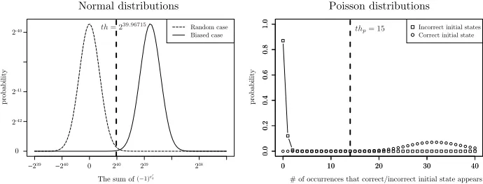
Fig. 2.Theoretical estimation for Example 2.
Proof. The total time complexity is estimated as
N+ (n−β)2n−β+m2n−β1+ (m2
p+m2m)2−β2.
In the useful attack parameter, since (m2
p+m2m)2−β2 is significantly smaller than the others, we regard it as negligible. We consider the case that other three terms are balanced, i.e.,
N = (n−β)2n−β=m2n−β1,
where1 is estimated as
1=√ 1
2πN Z ∞ th exp −x 2 2N
dx=1 2 ×erfc
th
√
2N
= n−β
m .
Thus, whenthis
th=√2N×erfc−1
2(n−β)
m
,
complexities of the three terms are balanced. We finally evaluate the probability that the initial state of the LFSR is uniquely recovered. The number of occurrences that each incorrect value appears follows the Poisson distribution with parameterλ1=N2−n. To discard all 2n−1 incorrect values, recallthp satisfyingP∞k=thp
λk
1e −λ1
k! <2−n. Then, the success probability is
P∞
k=thp λk
2e −λ2
k! whereλ2
is
λ2=m2−β2= m2
−β √ 2πN Z ∞ th exp
−(x−N c)
2 2N dx u t
Example 2. Let us consider an attack against an LFSR-based stream cipher with 80-bit LFSR. We assume that there are 214 linear masks whose correlation is greater than 2−36. For β = 9, we use N = (80−9)×280−9 ≈277.1498 parity-check equations. The left figure of Fig. 2 shows two normal
distributions: random and biased cases. If we use a following threshold
th=√2N×erfc−1
2(n−β)
m
≈239.9672,
1= (n−β)/m≈2−7.8503and2= 0.99957. The expected number of picked solutions is 280−91+
214−92 ≈263.1498+ 31.98627≈263.1498. We apply 214 inverse linear masks to the picked solutions
The number of occurrences that each incorrect value appears follows the Poisson distribution with parameter λ1 = 277.1498−80 = 2−2.8502. On the other hand, the number of occurrences that s(0) appears follows the Poisson distribution with parameterλ2= 214−9×0.99957≈31.98627. The
right figure of Fig. 2 shows two Poisson distributions. For example, whenthp= 15 is used, the prob-ability that an incorrect value appears at least 15 is smaller than 2−80. However, the corresponding
probability fors(0) is 99.9%. As a result, the total time complexity is 3×277.1498≈278.7348.
5
Application to Grain-128a
We apply the new algorithm to the stream cipher Grain-128a [˚AHJM11], which has two modes of operations: stream cipher mode and authenticated encryption mode. We assume that all output sequences of the pre-output function can be observed. Under the known-plaintext scenario, this assumption is naturally realized for the stream cipher mode because the output is directly used as a key stream. On the other hand, this assumption is very strong for the authenticated encryption mode because only even-clock output is used as the key stream. Therefore, we do not claim that the authenticated encryption mode can be broken.
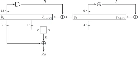
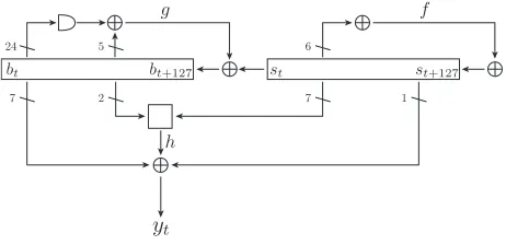
5.1 Specification of Grain-128a
yt
st st+127
bt bt+127
24 5
2
7 7 1
6
h
g f
Fig. 3.Specification of Grain-128a
Let s(t) and b(t) be 128-bit internal states of the LFSR and NFSR at time t, respectively, and s(t) andb(t)are represented ass(t)= (s
t, st+1, . . . , st+127) andb(t)= (bt, bt+1, . . . , bt+127). Letyt be an output of the pre-output function at timet, and it is computed as
yt=h(s(t), b(t))⊕st+93⊕
M
j∈A
bt+j, (2)
whereA={2,15,36,45,64,73,89}, andh(s(t), b(t)) is defined as
h(s(t), b(t)) =h(bt+12, st+8, st+13, st+20, bt+95, st+42, st+60, st+79, st+94)
=bt+12st+8⊕st+13st+20⊕bt+95st+42⊕st+60st+79⊕bt+12bt+95st+94. Moreover,st+128 andbt+128 are computed by
st+128=st⊕st+7⊕st+38⊕st+70⊕st+81⊕st+96,
bt+128=st⊕bt⊕bt+26⊕bt+56⊕bt+91⊕bt+96⊕bt+3bt+67⊕bt+11bt+13
⊕bt+17bt+18⊕bt+27bt+59⊕bt+40bt+48⊕bt+61bt+65⊕bt+68bt+84
⊕bt+88bt+92bt+93bt+95⊕bt+22bt+24bt+25⊕bt+70bt+78bt+82.
Let zt be the key stream at time t, and zt = yt in the stream cipher mode. On the other hand, in the authenticated encryption mode, zt = y2w+2i, where w is the tag size. Figure 3 shows the
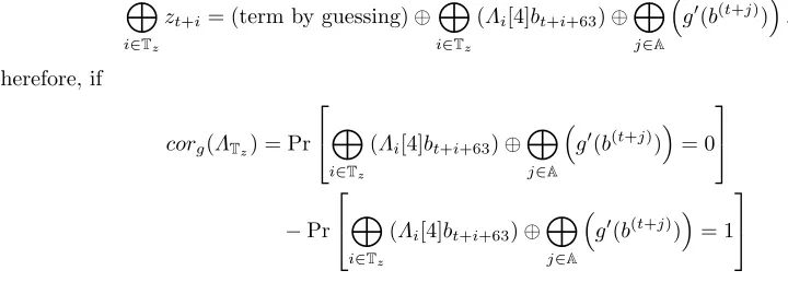
5.2 Linear Approximate Representation for Grain-128a
If there are multiple linear masks with high correlation, the new algorithm can be applied. In this section, we show that Grain-128a has many linear approximate representations, and they produce many linear masks.
93 94 79 60 42 95 20 13 8 12
g f
93 94 79 60 42 95 20 13 8 12
g f
93 94 79 60 42 95 20 13 8 12
g f n
n n
n
h
h
h
Fig. 4.Linear Approximate Representation for Grain-128a
Figure 4 shows the high-level view of the linear approximate representation. It involves fromtth to (t+n+ 1)th rounds, where b(t) and b(t+n+1) must be linearly inactive to avoid involving the
state of NFSR. Moreover,yt+i is linearly active fori∈Tz, and the linear mask of the input of the
(t+i)-roundhfunction denoted byΛi must be nonzero fori∈Tz. Otherwise, it must be zero.
We focus on the structure of the hfunction, where the input consists of 7 bits from the LFSR and 2 bits from the NFSR. Then, non-zeroΛi can take several values, and specifically,Λi can take 64 possible values (see Table 2) under the condition that a linear mask for 2 bits from NFSR is fixed. Since the sum of yt+i fori ∈Tz is used, it implies that there are 64|Tz| linear approximate representations. These many possible representations are obtained by exploiting the structure of the
hfunction, and this structure is common for all ciphers in the Grain family. In other words, this is a new potential vulnerability of the Grain family.
We first considerTzto construct the linear approximate representation, but it is difficult to find an optimalTz. Our strategy is heuristic and does not guarantee the optimality, but the foundTz is enough to break full Grain-128a. OnceTzis determined, we first evaluate the correlation of a linear approximate representation on fixed Λi fori∈ {0,1, . . . , n}. The high-biased linear maskγused in our new algorithm is constructed by Λi, and the correlation ofγ is estimated from the correlation ofΛi.
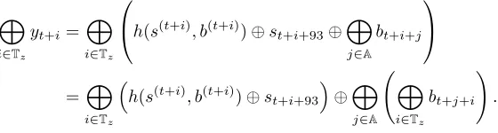
Finding Linear Masks with High Correlation. We focus on the sum of key stream bits, i.e.,
L
i∈Tzyt+i. From Eq. (2), the sum is represented as
M
i∈Tz
yt+i= M
i∈Tz
h(s
(t+i), b(t+i))⊕s
t+i+93⊕
M
j∈A
bt+i+j
=M
i∈Tz
h(s(t+i), b(t+i))⊕st+i+93
⊕M
j∈A M
i∈Tz
bt+j+i !
.
We first consider an appropriate setTz. We focus onLi∈Tzbt+j+iand chooseTzsuch that L
function, i.e.,Tz={0,26,56,91,96,128}. Then, for any j,
M
i∈Tz
bt+j+i=bt+j⊕bt+j+26⊕bt+j+56⊕bt+j+91⊕bt+j+96⊕bt+j+128
=st+j⊕g0(b(t+j)),
where
g0(b(t)) =bt+3bt+67⊕bt+11bt+13⊕bt+17bt+18⊕bt+27bt+59⊕bt+40bt+48
⊕bt+61bt+65⊕bt+68bt+84⊕bt+88bt+92bt+93bt+95
⊕bt+22bt+24bt+25⊕bt+70bt+78bt+82.
Note that all bits ing0(b(t)) are nonlinearly involved, and the correlation may be high. Then
M
i∈Tz
yt+i= M
i∈Tz
h(s(t+i), b(t+i))⊕st+i+93
⊕M
j∈A
st+j⊕g0(b(t+j))
=M
i∈Tz
st+i+93⊕
M
j∈A
st+j⊕ M
i∈Tz
h(s(t+i), b(t+i))⊕M
j∈A
g0(b(t+j)).
We next consider a linear approximate representation of h(s(t+i), b(t+i)). Let Λ
i ∈ {0,1}9 be the input linear mask for thehfunction at timet+i, andΛi= (Λi[0], Λi[1], . . . , Λi[8]). Then,
h(s(t+i), b(t+i))
≈Λi[0]bt+i+12⊕Λi[4]bt+i+95⊕ hΛi[1−3],(st+i+8, st+i+13, st+i+20)i
⊕ hΛi[5−8],(st+i+42, st+i+60, st+i+79, st+i+94)i,
whereΛi[x−y] denotes a sub vector indexed fromxth bit toyth bit. Letcorh,i(Λi) be the correlation of thehfunction at timet+i, and Table 2 summarizes them. From Table 2,corh,i(Λi) is 0 or±2−4.
We have 6 activehfunctions because|Tz|= 6, and letΛTz ∈ {0,1}
9×|Tz|be the concatenated linear mask, i.e., ΛTz = (Λ0, Λ26, Λ56, Λ91, Λ96, Λ128). The total correlation from all active h functions depends on ΛTz, and it is computed as corh(ΛTz) = (−1)
|Tz|+1Q
i∈Tzcorh,i(Λi) because of the piling-up lemma. Therefore, ifΛiwith correlation 0 is used for anyi∈Tz,corh(ΛTz) = 0. Otherwise,
corh(ΛTz) =±2
−24.
We guess all terms involved in the internal state of the LFSR in the FCA. Under the correlation
±2−24, we get
M
i∈Tz
yt+i≈(term by guessings(t))
⊕M
i∈Tz
(Λi[0]bt+i+12⊕Λi[4]bt+i+95)⊕
M
j∈A
g0(b(t+j)).
Therefore, if
corg(ΛTz) = Pr
M
i∈Tz
(Λi[0]bt+i+12⊕Λi[4]bt+i+95)⊕
M
j∈A
g0(b(t+j))= 0
−Pr
M
i∈Tz
(Λi[0]bt+i+12⊕Λi[4]bt+i+95)⊕
M
j∈A
g0(b(t+j))= 1
is high, the FCA can be successfully applied. Note thatcorg(ΛTz) is independent of Λi[1−3,5−8] for anyi∈Tz.
Appendix A shows the algebraic normal form of L j∈A g
0(b(t+j))
. To evaluate its correlation, we divide L
j∈A g
0(b(t+j))
Table 2.Correlation of thehfunction. The horizontal axis showsΛh,i[1−3], the vertical axis showsΛh,i[5−8],
and 512×corh,i is shown in every cell.
000 001 010 011 100 101 110 111 0000 -32 -32 -32 32 -32 -32 -32 32
0001 0 0 0 0 0 0 0 0
0010 -32 -32 -32 32 -32 -32 -32 32
0011 0 0 0 0 0 0 0 0
0100 -32 -32 -32 32 -32 -32 -32 32
0101 0 0 0 0 0 0 0 0
0110 32 32 32 -32 32 32 32 -32
0111 0 0 0 0 0 0 0 0
1000 -32 -32 -32 32 0 0 0 0
1001 0 0 0 0 -32 -32 -32 32
1010 -32 -32 -32 32 0 0 0 0
1011 0 0 0 0 -32 -32 -32 32
1100 -32 -32 -32 32 0 0 0 0
1101 0 0 0 0 -32 -32 -32 32
1110 32 32 32 -32 0 0 0 0
1111 0 0 0 0 32 32 32 -32
Case of
Λh,i[0,4] = 00.
000 001 010 011 100 101 110 111 0000 -32 -32 -32 32 -32 -32 -32 32
0001 0 0 0 0 0 0 0 0
0010 -32 -32 -32 32 -32 -32 -32 32
0011 0 0 0 0 0 0 0 0
0100 -32 -32 -32 32 -32 -32 -32 32
0101 0 0 0 0 0 0 0 0
0110 32 32 32 -32 32 32 32 -32
0111 0 0 0 0 0 0 0 0
1000 32 32 32 -32 0 0 0 0
1001 0 0 0 0 32 32 32 -32
1010 32 32 32 -32 0 0 0 0
1011 0 0 0 0 32 32 32 -32
1100 32 32 32 -32 0 0 0 0
1101 0 0 0 0 32 32 32 -32
1110 -32 -32 -32 32 0 0 0 0
1111 0 0 0 0 -32 -32 -32 32
Case of
Λh,i[0,4] = 01.
000 001 010 011 100 101 110 111 0000 -32 -32 -32 32 32 32 32 -32
0001 0 0 0 0 0 0 0 0
0010 -32 -32 -32 32 32 32 32 -32
0011 0 0 0 0 0 0 0 0
0100 -32 -32 -32 32 32 32 32 -32
0101 0 0 0 0 0 0 0 0
0110 32 32 32 -32 -32 -32 -32 32
0111 0 0 0 0 0 0 0 0
1000 -32 -32 -32 32 0 0 0 0
1001 0 0 0 0 32 32 32 -32
1010 -32 -32 -32 32 0 0 0 0
1011 0 0 0 0 32 32 32 -32
1100 -32 -32 -32 32 0 0 0 0
1101 0 0 0 0 32 32 32 -32
1110 32 32 32 -32 0 0 0 0
1111 0 0 0 0 -32 -32 -32 32
Case of
Λh,i[0,4] = 10.
000 001 010 011 100 101 110 111 0000 -32 -32 -32 32 32 32 32 -32
0001 0 0 0 0 0 0 0 0
0010 -32 -32 -32 32 32 32 32 -32
0011 0 0 0 0 0 0 0 0
0100 -32 -32 -32 32 32 32 32 -32
0101 0 0 0 0 0 0 0 0
0110 32 32 32 -32 -32 -32 -32 32
0111 0 0 0 0 0 0 0 0
1000 32 32 32 -32 0 0 0 0
1001 0 0 0 0 -32 -32 -32 32
1010 32 32 32 -32 0 0 0 0
1011 0 0 0 0 -32 -32 -32 32
1100 32 32 32 -32 0 0 0 0
1101 0 0 0 0 -32 -32 -32 32
1110 -32 -32 -32 32 0 0 0 0
1111 0 0 0 0 32 32 32 -32
Case of
Λh,i[0,4] = 11.
terms. Then we try out 4 possible values of (bt+67, bt+137) and evaluate correlation independently.
As a result, when (bt+67, bt+137) = (0,0) and (bt+67, bt+137) = (0,1), the correlation is −2−33.1875
and−2−33.4505, respectively. On the other hand, the correlation is 0 whenb
t+67= 1. Therefore
corg(ΛTz) =
−2−33.1875−2−33.4505
4 =−2
−34.313
whenΛi[0,4] = 0 for alli∈Tz.
We similarly evaluatecorg(ΛTz) whenΛi[0,4]6= 0 for anyi∈Tz. If one ofΛ0[0],Λ26[0],Λ56[0],
Λ91[4],Λ96[4], andΛ128[4] is 1, the correlation is always 0 becausebt+12,bt+38,bt+68,bt+186,bt+191,
andbt+223 are not involved toLj∈A g
0(b(t+j))
. Table 3 summarizescorg(ΛTz) whenΛ0[0],Λ26[0],
Λ56[0],Λ91[4],Λ96[4], andΛ128[4] are 0.
For any fixed Λi, we can get the following linear approximate representation
M
i∈Tz
yt+i ≈ M
i∈Tz
st+i+93⊕
M
j∈A
st+j⊕ M
i∈Tz
hΛi[1−3],(st+i+8, st+i+13, st+i+20)i
⊕M
i∈Tz
Table 3.Summary of correlations whenΛi[0,4] is fixed. Let∗be arbitrary bit.
Λ0[4]Λ26[4]Λ56[4]Λ91[0]Λ96[0]Λ128[0] corg(ΛTz)
0 0 0 0 0 0 −2−34.3130 0 0 0 0 0 1 +2−36.1875 0 0 0 0 1 0 −2−37.5860 0 0 0 0 1 1 +2−39.4605 0 0 0 1 0 0 −2−34.9230 0 0 0 1 0 1 +2−36.7975 0 0 0 1 1 0 +2−37.5860 0 0 0 1 1 1 −2−39.4605 0 0 1 0 0 0 −2−35.8980 0 0 1 0 0 1 +2−37.7724 0 0 1 0 1 0 −2−39.1710 0 0 1 0 1 1 +2−41.0454 0 0 1 1 0 0 −2−36.5080 0 0 1 1 0 1 +2−38.3825 0 0 1 1 1 0 +2−39.1710 0 0 1 1 1 1 −2−41.0454 0 1 0 0 0 0 −2−35.3636 0 1 0 0 0 1 +2−37.2381 0 1 0 0 1 0 −2−38.1710 0 1 0 0 1 1 +2−40.0454 0 1 0 1 0 0 −2−35.8490 0 1 0 1 0 1 +2−37.7235 0 1 0 1 1 0 +2−38.1710 0 1 0 1 1 1 −2−40.0454 0 1 1 0 0 0 −2−36.9486 0 1 1 0 0 1 +2−38.8230 0 1 1 0 1 0 −2−39.7559 0 1 1 0 1 1 +2−41.6304 0 1 1 1 0 0 −2−37.4340 0 1 1 1 0 1 +2−39.3085 0 1 1 1 1 0 +2−39.7559 0 1 1 1 1 1 −2−41.6304
1 ∗ ∗ ∗ ∗ ∗ 0
From the piling-up lemma, the correlation is computed as
−corg(ΛTz)×corh(ΛTz),
wherecorg(Tz) is summarized in Table 3 andcorh(ΛTz) = (−1)
|Tz|+1Q
i∈Tzcorh,i(Λi).
How to Find Multiple γ. The correlation of the linear approximate representation on fixed Λi
was estimated in the paragraph above. The linear maskγ used in the FCA directly is represented as
γ=X i∈Tz
Λi[1]αi+8+Λi[2]αi+13+Λi[3]αi+20+Λi[5]αi+42
+Λi[6]αi+60+Λi[7]αi+79+Λi[8]αi+94+αi+93
+X
j∈A
αj.
If differentΛTzs derive the sameγ, we need to sum up corresponding correlations.
Clearly, since this linear approximate representation does not involveΛi[0,4] fori∈Tz, we need
to sum up 22×|Tz|= 212 correlations, where Λi[1−3,5−8] is identical and only Λi[0,4] varies for
Moreover, there are special relationships. When we focus onΛ56[6] andΛ96[3], corresponding ele-ments over GF(2128) are identical becauseα56+60=α96+20=α116. In other words, (Λ56[6], Λ96[3]) =
(0,0) and (Λ56[6], Λ96[3]) = (1,1) derive the sameγ, and (Λ56[6], Λ96[3]) = (1,0) and (Λ56[6], Λ96[3]) = (0,1) also derive the sameγ. We have 3 such relationships as follows.
– Λ56[6] andΛ96[3]. Then,α56+60=α96+20=α116.
– Λ91[2] andΛ96[1]. Then,α91+13=α96+8=α104.
– Λ91[7] andΛ128[5]. Then,α91+79=α128+42=α170.
Therefore, from following three vectors
w1(δ[0]) = (09,09,000000100,000000000,000δ[0]00000,000000000), w2(δ[1]) = (09,09,000000000,001000000,0δ[1]0000000,000000000), w3(δ[2]) = (09,09,000000000,000000010, 000000000,00000δ[2]000),
a linear spanW(δ) = span(w1(δ[0]), w2(δ[1]), w3(δ[2])) is defined, whereδ[i] =δ[i]⊕1. As a result, the correlation forγ denoted bycorγ is estimated as
corγ = X
w∈W(δ)
X
v∈V
−corg(ΛTz⊕v)×corh(ΛTz⊕v⊕w).
Note thatcorg is independent ofw∈W(δ).
We heuristically evaluatedγ with high correlation. As shown in Table 2, the number of possible
Λi is at most 64. Otherwise,corh is always 0. Therefore, the search space is reduced from 254to 236. Moreover,Λ0is not involved inW(δ), and the absolute value ofcorγ is invariable as far as we useΛ0 satisfyingcorh,0=±2−4. Therefore, we do not need to evaluateΛ0anymore, and the search space is
further reduced from 236to 230. WhileΛ26is also not involved toW(δ), we have non-zero correlation
for both cases asΛ26[4] = 0 and 1 (see Table 3). If the sign ofcorh,26 forΛ26[4] = 0 is different from
that forΛ26[4] = 1, they cancel each other out. Therefore, we should useΛ26 such that the sign of correlation of Λ26 is equal to that of Λ26⊕(000010000), and the number of such candidates is 32. Then, we do not need to evaluate Λ26 anymore, and the search space is further reduced from 230
to 224. We finally evaluated 224 Λ
Tz exhaustively. As a result, we found 49152×64×32≈2
26.58γ
whose absolute value of correlation is greater than 2−54.2381.
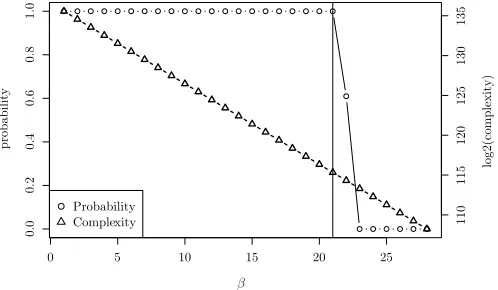
5.3 Estimation of Attack Complexity and Success Probability
0 5 10 15 20 25
0.0
0.2
0.4
0.6
0.8
1.0
β
probability
110
115
120
125
130
135
log2(complexity
)
Probability Complexity
We apply the attack algorithm described in Sect. 3, and Proposition 1 is used to estimate the at-tack complexity and success probability. Figure 5 shows the relationship between the time complexity, success probability, and the size of bypassed bits, where (n, m, c) = (128,49152×64×32,±2−54.2381)
is used. From Fig. 5,β= 21 is preferable. The time complexity is 3×(128−21)×2128−21≈2115.3264 and the corresponding success probability is almost 100%. Moreover when β = 22, the time com-plexity is 2114.3129 and the success probability is 60.95%.
The estimation above only evaluates the time complexity to recover the initial state of the LFSR. To recover the secret key, we need to recover the whole of the initial state. Our next goal is to recover the initial state of the NFSR under the condition that the initial state of the LFSR is uniquely determined, but it is not difficult. We have several methods to recover the initial state and explain the most simple method.
The key stream is generated as Eq. (2). We focus on (y0, . . . , y34), which involves 128 bits as (b2, . . . , b129). We first guess 93 bits, and the remaining 35 bits are recovered by using correspond-ing Eq. (2). Specifically, we first guess (b33, . . . , b75, b80, . . . , b129). Then, (b76, . . . , b79) are uniquely determined by using (y31, . . . , y34). Similarly, we can uniquely determine the remaining 31 bits step by step. While we need to guess 93 bits, the time complexity is negligible compared with that for the FCA.
6
Application to Grain-128
Grain-128 is the preliminary version of Grain-128a. The dynamic cube attack is successfully applied to analyze full Grain-128 and well exploits the low-degree feedback polynomial of NFSR. Actually, a higher degree feedback polynomial is adopted for Grain-128a to avoid the dynamic cube attack.
The FCA is absolutely different from the dynamic cube attack. While the dynamic cube attack analyzes the initialization, the FCA analyzes the key-stream generator. As far as we know, no vulnerability on the key-stream generator has been reported.
The specification is simpler than Grain-128a. The feedback polynomial of the NFSR is more sparse and is specified as
bt+128=st⊕bt⊕bt+26⊕bt+56⊕bt+91⊕bt+96⊕bt+3bt+67⊕bt+11bt+13
⊕bt+17bt+18⊕bt+27bt+59⊕bt+40bt+48⊕bt+61bt+65⊕bt+68bt+84.
Moreover there is a small tweak in thehfunction as
h(s(t), b(t)) =bt+12st+8⊕st+13st+20⊕bt+95st+42⊕st+60st+79⊕bt+12bt+95st+95,
wherest+95 is used instead ofst+94.
Since Grain-128 is very similar to Grain-128a, we can use the same Tz. Then−corg =−2−32, whereΛ26[4] andΛ91[0] can be chosen arbitrary but the others are 0.
We heuristically evaluated γ with high correlation, and we used the same strategy as the case of Grain-128a. As a result, we found 215×64×32 = 226 γ with correlation±2−51. We apply the
attack algorithm described in Sect. 3, and Proposition 1 is used to estimate the attack complexity and success probability. Figure 6 shows the relationship between the time complexity, success probability, and the size of bypassed bits, where (n, m, c) = (128,226,±2−51) is used. From Fig. 6, β = 22 is a
preferable attack parameter. The time complexity is 3×(128−22)×2128−22 ≈2114.3129 and the
corresponding success probability is 99.0%.
7
Application to Grain-v1
7.1 Specification of Grain-v1
Lets(t)andb(t)be 80-bit internal states of the LFSR and NFSR at timet, respectively, ands(t)and b(t)are represented as s(t)= (s
0 5 10 15 20 25
0.0
0.2
0.4
0.6
0.8
1.0
probability
110
115
120
125
130
135
log2(complexity
)
Probability Complexity
β
Fig. 6.Time complexity and success probability. FCA against Grain-128.
zt
st st+79
bt bt+79
13
1
7 4
6
h
g f
Fig. 7.Specification of Grain-v1
letztbe a key stream at timet, and it is computed as
zt=h(s(t), b(t))⊕ M
j∈A
bt+j, (4)
whereA={1,2,4,10,31,43,56} andh(s(t), b(t)) is defined as
h(s(t), b(t)) =h(st+3, st+25, st+46, st+64, bt+63)
=st+25⊕bt+63⊕st+3st+64⊕st+46st+64⊕st+64bt+63
⊕st+3st+25st+46⊕st+3st+46st+64⊕st+3st+46bt+63
⊕st+25st+46bt+63⊕st+46st+64bt+63.
Moreover,st+80 andbt+80 are computed by
st+80=st⊕st+13⊕st+23⊕st+38⊕st+51⊕st+62,
bt+80=st⊕bt+62⊕bt+60⊕bt+52⊕bt+45⊕bt+37⊕bt+33⊕bt+28⊕bt+21
⊕bt+14⊕bt+9⊕bt⊕bt+63bt+60⊕bt+37bt+33⊕bt+15bt+9
⊕bt+60bt+52bt+45⊕bt+33bt+28bt+21⊕bt+63bt+45bt+28bt+9
⊕bt+60bt+52bt+37bt+33⊕bt+63bt+60bt+21bt+15
⊕bt+63bt+60bt+52bt+45bt+37⊕bt+33bt+28bt+21bt+15bt+9
⊕bt+52bt+45bt+37bt+33bt+28bt+21.
Table 4.Correlation of thehfunction, where 32×corh,i is shown in every cell.
Λi[0−3]
0000 0001 0010 0011 0100 0101 0110 0111 1000 1001 1010 1011 1100 1101 1110 1111
Λi[4] = 0 0 0 0 0 0 -8 0 8 0 8 0 -8 -8 8 -8 8
Λi[4] = 1 0 -8 0 8 -8 -8 -8 -8 0 0 0 0 0 -8 0 8
7.2 Fast Correlation Attack against Grain-v1
When we use Tz ={0,14,21,28,37,45,52,60,62,80}, we focus on the sum of the key stream bits, i.e.,zt+0⊕zt+14⊕zt+21⊕zt+28⊕zt+37⊕zt+45⊕zt+52⊕zt+60⊕zt+62⊕zt+80.
M
i∈Tz
zt+i= M
i∈Tz
h(s(t+i), b(t+i))⊕M j∈A
M
i∈Tz
bt+j+i !
.
For anyj,
M
i∈Tz
bt+j+i=st+j⊕g0(b(t+j)),
whereg0(b(t)) is defined as
g0(b(t)) =bt+33⊕bt+9⊕bt+63bt+60⊕bt+37bt+33⊕bt+15bt+9⊕bt+60bt+52bt+45
⊕bt+33bt+28bt+21⊕bt+63bt+45bt+28bt+9⊕bt+60bt+52bt+37bt+33
⊕bt+63bt+60bt+21bt+15⊕bt+63bt+60bt+52bt+45bt+37
⊕bt+33bt+28bt+21bt+15bt+9⊕bt+52bt+45bt+37bt+33bt+28bt+21.
Then
M
i∈Tz
zt+i= M
i∈Tz
h(s(t+i), b(t+i))⊕M
j∈A
st+j⊕g0(b(t+j))
=M
j∈A
st+j⊕ M
i∈Tz
h(s(t+i), b(t+i))⊕M
j∈A
g0(b(t+j)).
We next consider a linear approximate representation of h(s(t+i), b(t+i)). Let Λ
i be the input linear mask for thehfunction at timet+i. Then
h(s(t+i), b(t+i))
≈Λi[4]bt+i+63⊕ hΛi[0−3],(st+i+3, st+i+25, st+i+46, st+i+64)i.
Letcorh,i(Λi) be the correlation of thehfunction at timet+i, and Table 4 summarizes them. From Table 4,corh,i(Λi) is 0 or±2−2. Since we have|
Tz|= 10 activehfunctions, the total correlation from all active hfunctions is computed as (−1)|Tz|+1Q
i∈Tzcorh,i(Λi) =±2
−20 because of the piling-up
lemma. Note thatΛi[0−3] is independent from the state of the NFSR.
All terms involved in the internal state of the LFSR can be guessed in the FCA. Therefore, under the correlation±2−20, we get
M
i∈Tz
zt+i= (term by guessing)⊕ M
i∈Tz
(Λi[4]bt+i+63)⊕
M
j∈A
g0(b(t+j)).
Therefore, if
corg(ΛTz) = Pr
M
i∈Tz
(Λi[4]bt+i+63)⊕
M
j∈A
g0(b(t+j))= 0
−Pr
M
i∈Tz
(Λi[4]bt+i+63)⊕
M
j∈A
g0(b(t+j))= 1
Table 5.Summary of correlations whenΛi[4] is fixed.
Λ14[4]Λ21[4]Λ28[4]Λ45[4] corg(ΛTz)
0 0 0 0 −2−39.7159 0 0 0 1 −2−43.4500 0 0 1 0 −2−39.6603 0 0 1 1 −2−43.7260 0 1 0 0 +2−45.1228 0 1 0 1 −2−42.9025 0 1 1 0 +2−44.3802 0 1 1 1 −2−42.6875 1 0 0 0 +2−41.9519 1 0 0 1 +2−43.5233 1 0 1 0 +2−41.8662 1 0 1 1 +2−43.6420 1 1 0 0 −2−44.9114 1 1 0 1 +2−42.8544 1 1 1 0 −2−44.5232 1 1 1 1 +2−42.7302
is high, the FCA can be successfully applied.
Similarly to the case of Grain-128a, we evaluatecorg(ΛTz). If one ofΛ0[4],Λ37[4],Λ52[4],Λ60[4],
Λ62[4], and Λ80[4] is 1, the correlation is always 0 becausebt+63, bt+100, bt+115,bt+123, bt+125, and bt+143 are not involved in Lj∈A g
0(b(t+j))
. Table 5 summarizes corg(ΛTz) when Λi[4] = 0 for
i∈ {0,37,52,60,62,80}.
For any fixed Λi, we can get the following linear approximate representation
M
i∈Tz
zt+i≈ M
j∈A
st+j⊕ M
i∈Tz
hΛi[0−3],(st+i+3, st+i+25, st+i+46, st+i+64)i. (5)
From the piling-up lemma, the correlation is computed as−corg(ΛTz)×corh(ΛTz).
How to Find Multiple γ. The correlation of the linear approximate representation on fixed Λi
was estimated in the paragraph above. The linear maskγ used in the FCA directly is represented as
γ=X i∈Tz
Λi[0]αi+3+Λi[1]αi+25+Λi[2]αi+46+Λi[3]αi+64
+X
j∈A
αj.
If differentΛh have the sameγ, we need to sum up corresponding correlations.
This linear approximate representation does not useΛi[4] for i∈Tz. Therefore, we need to sum
up 2|Tz|= 210 correlations, whereΛi[0−3] is identical and onlyΛi[5] varies fori∈
Tz. LetV be a
linear span whose basis is 12 corresponding unit vectors.
Moreover, there are special relationships similar to the case of Grain-128a, and we have four such relationships as
– Λ37[2] andΛ80[0]. Then,α37+46=α80+3=α83.
– Λ62[3] andΛ80[2]. Then,α62+64=α80+46=α126.
– Λ0[2] andΛ21[1]. Then,α0+46=α21+25=α46.
– Λ21[3] andΛ60[1]. Then,α21+64=α60+25=α85.
Therefore, from following four vectors
5 10 15
0.0
0.2
0.4
0.6
0.8
1.0
β
probability
70
75
80
85
log2(complexity
)
Probability Complexity
Fig. 8.Time complexity and success probability. FCA against Grain-v1.
a linear span W(δ) = span(w1(δ[0]), w2(δ[1]), w3(δ[2]), w4(δ[3])) is defined, where δ[i] = δ[i]⊕1. Then, letcorγ be the correlation ofγ, and
corγ = X
w∈W(δ)
X
v∈V
−corg(ΛTz⊕v)×corh(ΛTz⊕v⊕w).
We heuristically evaluated γ with high correlation. For every element in Tz, since the subset {14,28,45,52}is independent of the special relationship, we first focus on the subset. Sincebt+63+52
is not involved inL j∈A g
0(b(t+j))
, Λ52[4] must be 0. Therefore,Λ52[0−3] should be chosen as
Λ52[0−3]∈ {0101,0111,1001,1011,1100,1101,1110,1111},
and corγ is invariable as far as we use Λ52 satisfyingcorh,52 =±2−2. We do not need to evaluate Λ52 anymore, and the search space is reduced from 240 to 236. Fori ∈ {14,28,45}, corresponding
masks should be chosen as
Λi[0−3]∈ {0101,0111,1001,1011,1100,1101,1110,1111}
becausecorg(ΛTz) is high when (Λ14[4], Λ21[4], Λ28[4], Λ45[4]) is 0010 or 0000. Let us focus on Table 5. We have three-type linear masks as
– Λi[0−3] ∈ {1001,1011,1100,1110}, where corh,i = ±2−2 for Λi[4] = 0 but corh,i = 0 for
Λi[4] = 1.
– Λi[0−3]∈ {0111,1101}, where the sign ofcorh,i is different in each case ofΛi[4] = 0 or 1. – Λi[0−3]∈ {0101,1111}, where the sign ofcorh,i is the same in both cases ofΛi[4] = 0 and 1.
Since corγ is invariable in each case, it is enough to evaluate one from each case. Therefore, the search space is reduced from 236 to 33×224. We finally evaluated 9×224 Λ
Tz exhaustively. As a result, we found about 442368γ whose absolute value of correlation is greater than 2−36.
Estimating Attack Complexity and Success Probability. We apply the attack algorithm
described in Sect. 3, and Proposition 1 is used to estimate the attack complexity and success proba-bility. Figure 8 shows the relationship between the time complexity, success probability, and the size of bypassed bits, where (n, m, c) = (80,442368,±2−36) is used. From Fig. 8,β = 11 is preferable, and
the time complexity is 3×(80−11)×280−11 ≈276.6935 and the corresponding success probability
0 10 20 30 40
0.0
0.2
0.4
0.6
0.8
Theoretical and experimental simulations
# of occurrences that correct/incorrect initial state appars
pr
obability
Incorrect initial states (theoretical) Correct initial state (theoretical) Incorrect initial state (experimental) Correct initial state (experimental)
thp= 9
Fig. 9.Comparison between the theoretical and experimental estimations.
8
Verifications, Observations, and Countermeasures
8.1 Experimental Verification
We verify our algorithm by applying it to a toy Grain-like cipher, where the sizes of the LFSR and NFSR are 24 bits, andst+24,bt+24, andztare computed as
st+24=st⊕st+1⊕st+2⊕st+7,
bt+24=st⊕bt⊕bt+5⊕bt+14⊕bt+20bt+21⊕bt+11bt+13bt+15,
zt=h(st+3, st+7, st+15, st+19, bt+17)⊕
M
j∈{1,3,8} bt+j,
where thehfunction is as the one used in Grain-v1.
Similarly to the case of Grain-128a,Tzis used by tapping linear part of the feedback polynomial of NFSR, i.e.,Tz={0,5,14,24}. Then, the sum of the key stream is
M
i∈Tz
zt+i = M
i∈Tz
h(s(t+i), b(t+i))⊕ M
j∈{1,3,8}
st+j+g0(b(t+j))
,
where g0(b(t)) = b
t+20bt+21⊕bt+11bt+13bt+15. The ANF of the h function involves bt+17, bt+22, bt+31, and bt+41. If Λi[4] = 1 is used for i ∈ {0,14,24}, the correlation is always 0 because
L
j∈{1,3,8}g0(b(t+j)) does not involvebt+17,bt+31, andbt+41. Onlybt+22is involved toLj∈{1,3,8}g0(b(t+j)).
Therefore, we evaluated correlations of L
j∈{1,3,8}g0(b(t+j)) and
L
j∈{1,3,8}g0(b(t+j))⊕bt+22, and
they have the correlation 2−3.41504. For i ∈ {0,14,24}, we have 8 possible linear masks. Moreover,
we should use 0101 and 1111 for the linear mask Λ14[0−3] because the sign of the correlation is the same in either case of Λ14[4] = 0 and Λ14[4] = 1. As a result, we have 8×8×8×2 = 1024 linear masks whose absolute value of correlations is 2×2−8−3.41504= 2−10.41504, where the factor 2
is derived from the sum of correlations forΛ14[4] = 0 andΛ14[4] = 1.
For example, whenβ = 5, the data complexity is (24−5)×224−5≈223.25. From Proposition 1,
when we useth= 6579 as the threshold for the normal distribution, the complexities for three steps of the attack algorithm are balanced. Moreover, when we usethp= 9 as the threshold for the Poisson distribution, the probability that incorrect initial state appears at leastthp times is 2−26<2−24.
We randomly choose the initial state and repeat the attack algorithm 1000 times. Figure 9 shows the comparison of the Poisson distributions between the theoretical and experimental ones. From this figure, our experimental results almost follow the theoretical one.
8.2 Unified Representation with Finite Field
The “commutative” property of Γ ×TFt is exploited in our new fast correlation attack, where
:n-bit row vector :n n-bit matrix :n-bit column vector
commutative Ft
s(0)
τ(s(0))
Fig. 10.“Commutative” property
Recall Eq.( 1), the parity-check equation is represented as
e0t= D
s(0), Γ×TFtE⊕M
i∈Tz
zt+i
=s(0)×Ft×TΓ⊕M i∈Tz
zt+i.
We equivalently transformFt×TΓ intoαtγin our new algorithm. We further consider the equivalent representation ofs(0) over GF(2n), which is denoted byτ(s(0)), and Eq.( 1) is rewritten as
e0t= (τ(s(0))γαt)[0]⊕ M
i∈Tz
zt+i,
where (τ(s(0))γαt)[0] is the first coefficient ofτ(s(0))γαt, and Fig. 10 shows the overview.
The conversion functionτ :{0,1}n→GF(2n) is a bit trickier than conversions forFtandΓ. It is not natural becauses(0) is ann-bitrowvector, and therefore, we need to introduce a conversion
functionτ as follows.
Definition 2 (Conversion function τ). For any y ∈ GF(2n), let us consider an n×n matrix
[y, αy, α2y, . . . , αn−1y]. Thenτ−1(y)is the first rown-bit vector in this matrix, andτ is the inversion
of τ−1.
The following is an example in the case of GF(28) = GF(2)[x]/(x8+x4+x3+x2+ 1).
Example 3. We consider the conversion τ for GF(28) = GF(2)[x]/(x8+x4+x3+x2+ 1). When y = α(= 01000000) and y = α+α3+α4+α6+α7(= 01011011), the first row of the matrix [y, αy, α2y, . . . , α7y] is 00000001 and 01101001, respectively, because
0 0 0 0 0 0 0 1 1 0 0 0 0 0 0 0 0 1 0 0 0 0 0 1 0 0 1 0 0 0 0 1 0 0 0 1 0 0 0 1 0 0 0 0 1 0 0 0 0 0 0 0 0 1 0 0 0 0 0 0 0 0 1 0
and
0 1 1 0 1 0 0 1 1 0 1 1 0 1 0 0 0 0 1 1 0 0 1 1 1 1 1 1 0 0 0 0 1 0 0 1 0 0 0 1 0 1 0 0 1 0 0 0 1 0 1 0 0 1 0 0 1 1 0 1 0 0 1 0
.
Thereforeτ(00000001) =α= 01000000 andτ(01101001) =α+α3+α4+α6+α7= 01011011.
8.3 Experimental Path Search Algorithm
An unified representation with the finite field is shown in Sect. 8.2, where s(0) is also represented
![Table 2. Correlation of the h function. The horizontal axis shows Λh,i[1−3], the vertical axis shows Λh,i[5−8],and 512 × corh,i is shown in every cell.](https://thumb-us.123doks.com/thumbv2/123dok_us/7980550.1323668/14.612.120.498.106.476/table-correlation-function-horizontal-shows-vertical-shows-shown.webp)
![Table 3. Summary of correlations when Λi[0, 4] is fixed. Let ∗ be arbitrary bit.](https://thumb-us.123doks.com/thumbv2/123dok_us/7980550.1323668/15.612.203.409.92.467/table-summary-correlations-li-xed-let-arbitrary-bit.webp)