ISSN (e): 2250-3021, ISSN (p): 2278-8719
Vol. 06, Issue 07 (July. 2016), ||V2|| PP 48-56
Improved Signal Processing and Calibration Methods for GPR
Tomography
Yasar Guzel
1, Ali Nassib
21University of Dayton
2University of Dayton
Abstract
: -A fast matched-filter reconstruction technique for ground penetrating radar (GPR) tomography is proposed for generating 2D images of buried objects with signal processing techniques to calibrate GPR data. Reconstruction of a 2D image from these data is achieved with numerical discretization and matched-filter techniques. This requires less computational power and is simpler to implement relative to matrix inversion or other inversion methods. The primary benefits, as compared to other GPR imaging methods, are improved resolution and 2D imaging for easy survey analysis. The 2D imaging benefits are derived from the increased data collection (via multiple antenna look) that supports state-of-the-art GPR tomography to generate high-resolution 2D images. In addition, background suppression and calibration methods are presented to further the technique by removing clutter. Experimentation at the Mumma Radar Lab (MRL) at the University of Dayton was conducted to verify the proposed technique.Keywords: -
Born approximation, Calibrations, Ground penetrating radar, Radio frequency, Matched-filter,
Tomography.I.
INTRODUCTION
Ground penetrating radar (GPR) transmits electromagnetic (EM) waves into the ground and uses the reflected signals to develop a map of subsurface structures. Applications of this technology include locating buried infrastructure such as pipes and cables, landmines[1][2] and tunnels[3], identifying explosive devices, and imaging archaeological artifacts. Depending on the configuration of transmitters and receivers, GPR devices can map subsurface structures in a single dimension or it can create higher dimensional imagery. In all cases, a buried object scatters incident radiation in proportion to its radar cross section, and the reflected signal carries quantitative information about the object’s size, shape and location relative to the transmitting and receiving antennas. The reflected signal, which is often collected by moving the receiving antenna over a rectangular grid, also contains ground echo, noise and clutter. This work explores GPR tomography, which is a variation of the technology that extracts greater information from the reflected signals in order to create two-dimensional images.
In order to increase the resolution and generate high resolution images, GPR Tomography processes the phase measurement data topographically (i.e., from a variety of viewing angles). The data is then adaptively combined coherently to produce the high-resolution image. A major advantage of the proposed adaptive tomographic signal processing techniques is that the target is viewed from multiple look angles, which overcomes the effect of dominant scattering (strong reflections) from the front surfaces (leading edges) of the target and subsequent shadowing (weak reflections) from the back surfaces of the target. The composite image formed by combining (topographically) the scattered data from multiple look angles produce a full image of the target and is much more detailed than the individual images formed from only one of the single angle data sets. These improvements are not feasible with traditional wideband GPR SAR approaches. In addition, the resolution of the target image is enhanced as a result of the multi-static tomographic signal processing. This allows an improved resolution using a given frequency at a given depth.
II.
GPR TOMOGRAPHY SIGNAL MODEL
The GPR tomography scenario considered in this work is illustrated in Fig.1. Transmitter (TX) is located above the ground and placed at position, t
n
r and receiver RX (receiver) placed at positionrmr. The direction for TX’s and RX’s are represented by vectors ˆt
n
a andaˆrm, respectively. The total field Et o tcan be expressed in terms of the incident field, i n
E , and scattered field,
t o t in s c
E = E + E (1)
The incident electric field is given by [4]
Ein j G r( nt,r) (2) where G r( nt,r) is the Dyadic Green’s function corresponding to the electromagnetic wave at the target position
r due to a wave originated from rnt .
Scattered field received from the antenna in frequency domain is [5]
Es c(, rnt,rmr) =
G (,r , r ) v ( r ) E mr to t(, r) d r (3) wherev ( r ) is the reflectivity function, which determines if the target is present in the region D. The scattered field s cE cannot be solved from this equation because Es c is included inEt o t. Moreover, both v ( r ) is and,Es c, are unknown that are, contained within t o t
E .This problem occurs in many remote-sensing and imaging situations, and they generally involve the reconstruction of a reflectivity function from the scattered field created by the presence of an object. Although this is a non-linear process, the Born approximation is often used in the case of weak scatterers in order to simplify the description of inverse-scattering problems and to improve computational efficiency in solving them. This leads to linear inverse-scattering theory, which is often used to solve free-space and half-space problems for homogenous media and inhomogeneous layered media [6][7][8]. A first-order Born approximation assumes that the scattered and incident radiation have the same amplitude, but different directions. Higher order, extended Born approximations with closed-form relationships to linear inverse scattering are possible, but these are computationally expensive and difficult to implement[9][10].
The Born approximation can be applied to the total electric field on the right hand side of Equation (3) .To linearize Equation (3) , t o t
E replaced with the known incident field, i n
E . This leads to simplified equation
(, nt, mr)
, (, )d s c r in
m
r r r
E G ( r , r ) v ( r ) E r (4) Substituting Equation (2) into Equation
(, nt, mr)
, , s c t r
n m
E r r G ( r , r ) G ( r , r ) v ( r ) d r (5) To reconstruct the image of buried object, the region D is discretized and divided into P voxels. The scattered electric field received from the target is
n m n m p p
E L v (6)
whereEn mis the scattered electric fields samples, and the reflectivity function,
n m p
L is multiplication of the
scattered electric field due to the t h
n transmitter and t h
m receiver for the th
p voxel location, The row vector,vp , has length P, and if there is no target present at voxel p , then vp 0 , p 1 . . .P . On the contrary, if a target
is present, an isotropic scattered wave is generated with reflectivity function[11].
All experimental data is recorded with VNA (Vector Network Analyzer) which saves the data in real and imaginary parts(S-parameters). The S-parameters are proportional to the scattered electric fields [12], and Equation (6) becomes
sL v . (7)
An image is reconstructed by solving for v through matrix inversion. However, the matrix L may not be invertible. The received data contains target information and noise. The s vector can be written in terms of the white Gaussian noise (rn m p) and scattered field (ln m pvp ).
s rn m pIn m pvp (8) The usual way to solve Equation (7) is by using a Hermitian matrix inversion method. Alternatively, a matched filter method can be applied to estimate the vector. Finding a new vector y in Equation (9) is equivalent to vectorv.
y LH s. (9)
Assume a single point target is present at p1 in region D, with a corresponding reflectivity function for this voxel of v1 1 and vp 0 forp 2 , 3 ,P, such that
1 1 2 2 1 1 1 1. 0
n m v n m v n m PvP n m n m v n m
s l l l r l r
(10)
In order to maximize the SNR, a matched filter H
w can be applied to s such that
1 H 1 1.
n m H
y w s w l v (11) Finding the unknown matched filter H
w solves the imaging problem by approximating the output y1 in Equation (11). After applying the filter H
w , the SNR is
2
1 1
2
1
S N R ,
H n m H n m v E w l w r (12)
SNR is maximized when w ln m1 , and the value of y1 is therefore estimated by 1 1
H n m
y LH s. (13) Image formation can now be accomplished through y via Equation (13). This result can also be achieved by applying matrix inversion algorithms.
III.
REMOVING THE CLUTTER
The back-scattered signal includes unwanted clutter mixed with target of interest. Background subtraction is a technique to eliminate incident field without erasing the target that is embedded inside back-scattered signal. Background subtraction is applied to each A scan data collections, and the averaged value of the ensemble of A scans subtracted is given by following equation [13].
, , , 1
1
( ) ( ) ( )
k
n m n m n m
m
B t B t B t
k
(14)where n is number of the A scan,k is the number of the sample in each A scan, Bn m, is A scan data vector, andBn m, is processed A scan vector.
To extract target information from the received signal, the direct path effects should be minimized. The GPR systems record the transmitted signal from different paths. The coupling between transmitters and receivers is
the biggest challenge to be overcome. One of the solution to overcome this problem is to activate different transmitters and analyze their current distribution in order to place electric field nulls at the desired transmitter
or receiver location [14].This approach is not easy to implement. The direct path may mask the targets if the
distance between two antennas is equal to or greater than the bistatic range.
Proper shielding may also reduce direct path effects [15], but it is not an preferred method .One way to record the direct path is by pointing the antennas to each other as illustrated in Figure 2. First data are collected when antennas are pointed to the area of interest (see Figure 2 (a)).
(a)
Fig. 2Direct path removal: (a) antennas pointed to area of interest and (b) antennas pointed to each other
Then data is recorded when antenna pointed to each other (see Figure 2 (b)). The background is collected at each step and subtracted for both data sets.The direct path can be removed by applying
( 2 1 )
( ) d ir e c t
r e m o v e d b k g
j k
e
R R2 1
2 1 2 1 2 1
S S S (15) where
r e m o v e d 2 1
S is the direct path removed of scattering parameters,
b k g 2 1
S is the background , S2 1 is the scattering parameters,R2 1 is distance where the peak value appears in the range profile, and 2 1d i r e c t
R is
distance where the peak value appears in the direct path range profile.
IV.
ANTENNA CALIBRATION
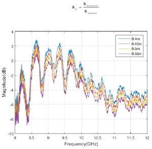
The antenna calibration technique serves to remove the clutter from measured GPR data. An antenna aperture optimization, antenna phase center estimation, and determination of the antenna transfer function are all parts of the antenna calibration procedure. These procedures are explained in [16], [17]. The received waveform is distorted due to the frequency characteristic of the GPR antenna [18]. To eliminate this distortion in the measured GPR data, normalization is used to extract the transfer function of the scene[19]. The frequency domain measurement is the product of the frequency transfer function as well as the frequency response of the target scene. In order to extract the transfer function of the scene only, the measured transfer function must be divided by the transfer function of the antennas
m e a s u r e d tf
a n te n n a
S
S S
(16)
where St f is transfer function of the scene,Sm e a s u r e d is the measured transfer function, and Sa n te n n a is the transfer function of the antenna.
The transfer function of the antennas (together) was measured by pointing them at each other and recording S21 on the VNA (see Figure 2 (b)). This was done at different distances to investigate the effect of the possible multiple reflections and near-field effects. The antenna transfer function is recorded from 8 to 12GHz with 16001 points. Fig shows the S21 measurements at separations from 0.4 meter to 0.55 meter. In the experiments reported here, the 0.55 meter response was used for calibration. The collected GPR data are normalized by the
V.
FLAT METAL PLATE CALIBRATION
The plate calibration was used as a calibration object because it is affordable and the received signal is well known. Range is very important in determining wave propagation velocity and target location. The plate calibration technique improves the accuracy of range estimation [20]. To calibrate the GPR systems, two bistatic antennas are pointed to metal plate, 58feet, (see Figure 4 (a)). The pins of the antenna are parallel to the plane of the flat plate, and the distance between the each antenna and the metal flat plate is 1 meter.
Two port VNA calibration is performed before any data collections. The background is recorded and the background subtraction technique is applied to the recorded metal plate data. A scan data is collected at 161 locations. The metal flat plate response is a flat line at 1 meter (see Figure 4 (b)).
VI.
EXPERIMENTATION
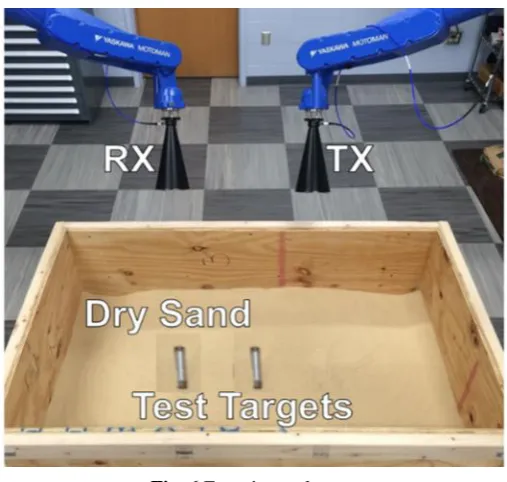
As presented in Figure 5, the Mumma Radar Lab (MRL) is equipped with four robotic arms, each one having a dual polarized horn antenna operating up to 18 GHz, and a central turntable which rotates at variable yet controlled rate. The four robotic arms and turntable operate under the control of a single, integrated processor. The MRL is developing GPR Tomography technology and a capability to emulate the effects of motion in both SAR and ISAR. At the heart of the system is the software MATLAB running on a high-powered computer with two Intel Xeon quad-core processors and 128 GB DDR3 RAM. This software is in charge of controlling the Motoman robot movements to scan the scene of interest, requesting and recording data from the Agilent vector network analyzer (VNA), processing captured data, and producing the final image.
(a)
(b)
Fig. 5 Mumma Radar lab
Two targets includes pair of 5 inch long metal pipes with half inch radius that are vertically buried into dry sand. The base of the pipes are located at (x, y, z) = (5, -5, -25) cm and (x, y, z) = (10, 5,-25) cm below from the surface of the sand. The antennas move on square grid 0 .60 .6 meter, following a linear path on the grid
with 2 cm step size. The distance between the antennas is 70 cm, measured aperture center of antennas. The height of each antenna from the sand is 20 cm. The data are recorded for a frequency range of 8 to 12 GHz. The process is repeated with the two targets absent, to perform background subtraction, and mitigate interference. A total of 16001 frequency samples are collected at each point on the grid. Data is calibrated and direct path effects is removed as explained in section 3, section 4, and section 5. Data are processed and the image is formed as shown in Fig (a) which is indicating location of the pipes and Figure (b) shows shape of the pipes.
VII.
CONCLUSION
This paper presented a fast matched-filtered method to image below ground object by applying signal processing techniques, and calibration methods to calibrate GPR data for GPR tomography application. The techniques serve to detect, image, and estimate the position of buried objects. Noise and clutter are the most significant irregularities present during GPR raw data collection. Eliminating these types of irregularities is achieved with pre-processing by applying calibration methods to achieve better accuracy.
For future work, different trajectories can be applied to maximize perspective of diversity while keeping number of the scan points. Also, the algorithms can be tested for wet sand and other inhomogeneous mediums.
VIII.
ACKNOWLEDGMENT
This research was funded, in part, by the Ohio Third Frontier Ohio Research Scholars Program, the University of Dayton Department Of Electrical and Computer Engineering, and Dr. Nagu V. Nagarajan, President of RNET Technologies. Their support is deeply appreciated.
IX.
REFERENCES
[1] K. H. Ko, G. Jang, K. Park, and K. Kim, “GPR-Based Landmine Detection and Identification Using Multiple Features,” Int. J. Antennas Propogations, vol. 2012, 2012.
[2] A. Dyana, C. H. S. Rao, and R. Kuloor, “3D Segmentation of Ground Penetrating Radar Data for Landmine Detection,” in 14th International Conference on Ground Penetrating Radar (GPR), 2012, pp. 858–863.
[3] M. C. Wicks, “RF Tomography with Application to Ground Penetrating Radar,” in Signals, Systems and Computers, 2007. ACSSC 2007. Conference Record of the Forty-First Asilomar Conference on, 2007, pp. 2017–2022.
[4] T. J. Cui and W. C. Chew, “Diffraction Tomographic Algorithm for the Detection of Three-dimensional Objects Buried in a Lossy Half-Space,” IEEE Trans. Antennas Propag., vol. 50, no. 1, pp. 42–49, 2002. [5] L. Lo Monte, D. Erricolo, F. Soldovieri, and M. C. Wicks, “Radio Frequency Tomography for Tunnel
Detection,” IEEE Trans. Geosci. Remote Sens., vol. 48, no. 3, pp. 1128–1137, 2010.
[6] B. Hu and W. C. Chew, “Fast inhomogeneous plane wave algorithm for scattering from objects above the multilayered medium,” IEEE Trans. Geosci. Remote Sens., vol. 39, no. 5, pp. 1028–1038, 2001.
[7] N. Geng, A. Sullivan, and L. Carin, “Multilevel Fast-multipole Algorithm for Scattering from Conducting Targets Above or Embedded in a Lossy Half Space,” IEEE Trans. Geosci. Remote Sens., vol. 38, no. 4 I, pp. 1561–1573, 2000.
[8] T. J. Cui, Y. Qin, Y. Ye, J. Wu, G. Wang, and W. C. Chew, “Efficient Low-Frequency Inversion of 3-D Buried Objects with Large Contrasts,” vol. 44, no. 1, pp. 3–9, 2006.
[9] T. J. Cui, Y. Qin, Y. Ye, J. Wu, G. L. Wang, and W. C. Chew, “High-order Inversion Formulas for 3D Buried Dielectric Objects,” in IEEE Antennas and Propagation Society, AP-S International Symposium (Digest), 2005.
[10] M. Almutiry, M. C. Wicks, A. Nassib, and L. Lo Monte, “Extraction of Weak Target Features from Radar Tomographic Imagery,” in IEEE NAECON National Aerospace & Electronics, 2015, pp. 194–197. [11] T. M. Tran, “Passive RF Tomography:Signal Processing and Experimental Validation,” Air Force
Institute of Technology, 2014.
[12] S. Arslanagi, T. V. Hansen, N. A. Mortensen, A. H. Gregersen, O. Sigmund, R. W. Ziolkowski, and O. Breinbjerg, “A Review of the Scattering-parameter Extraction Method with Clarification of Ambiguity Issues in Relation to Metamaterial Homogenization,” IEEE Antennas Propag. Mag., vol. 55, no. 2, pp. 91–106, 2013.
[13] David J.Daniels, Ground Penetrating Radar. IET, 2004.
[14] L. Lo Monte, L. K. Patton, and M. C. Wicks, “Mitigation of Coupling in RF Tomography with Applications to Belowground Sensing,” in IEEE National Radar Conference, 2010, pp. 215–219.
[15] C. Chen, “Fully-Polarimetric Ground Penetrating Radar Application,” in Antennas and Propagation Society International Symposium, 2001, vol. 4, pp. 604–607.
[16] K. Z. Jadoon, S. Lambot, E. C. Slob, and H. Vereecken, “Analysis of Horn Antenna Transfer Functions and Phase-Center Position for Modeling Off-Ground GPR,” IEEE Trans. Geosci. Remote Sens., vol. 49, no. 5, pp. 1649–1662, May 2011.
[17] G. G. Gentili and U. Spagnolini, “Electromagnetic Inversion in Monostatic Ground Penetrating Radar : TEM Horn Calibration and Application,” IEEE Trans. Geosci. Remote Sens., vol. 38, no. 4, pp. 1936– 1946, 2000.
[18] M. Nishimoto, D. Yoshida, K. Ogata, and M. Tanabe, “Target Response Extraction from Measured GPR Data,” in Antennas and Propagation (ISAP), International Symposium on, 2012, pp. 427–430.
[19] L. L. Grootboom and A. J. Wilkinson, “Fine Resolution(1.25 cm) Ultra Wideband Radar Tomographic Imaging Using 8.5GHz Vector Network Analyzer and a Rotating Pedestral,” in IEE International Radar Conference, 2015, pp. 4–7.