Approach
Thesis by Peyman Tavallali
In Partial Fulfillment of the Requirements for the Degree of
Doctor of Philosophy
California Institute of Technology Pasadena, California
2014
© 2014
Acknowledgements
I need to express my deepest gratitude to my research adviser, Prof. Thomas Y. Hou, for his support, encouragement, and guidance throughout my Ph.D. re-search journey at Caltech. I have benefited greatly from his broad and deep insight into mathematics. I especially need to thank him for introducing me to the area of multiscale-adaptive data analysis, which led to the research in the topic of this thesis. I am grateful to many other academic members and advisors. I would like to thank Dr. Mojtaba Mahzoon, my research and life adviser during my B.Sc. degree at Shiraz University, for his friendship, mentorship, and for introducing me to the interesting and charming field of applied mathematics. His logical advice helped me to overcome my uncertainty about continuing my studies outside of my home country. His words are always moral guidance for me. I am also grateful to Prof. Vladimir V. Kulish, my research adviser in Singapore, for his support during my stay in Nanyang Technological University. I would like to thank Prof. Morteza (Mory) Gharib, who gave me the opportunity to work on biological signals using our newly developed sig-nal processing method, which resulted in some interesting interdisciplinary research results that could be used to save thousands of lives.
I want to thank Professors Thomas Y. Hou, Houman Owhadi, James L. Beck , and Mory Gharib whose comments as members of my dissertation committee were extremely valuable to my research.
Niema and me develop our ideas. I would also like to thank Dr. Zuoqiang Shi for helping me understand many aspects of signal processing, giving me a deeper under-standing of the topics in my dissertation. Furthermore, I am grateful to him for our satisfying collaboration which led to indepth publications on some of the topics from my dissertation. Finally, I thank my collegue Diane Guignard for helping me through some challenging problems while she worked on her Master’s dissertation at Caltech. I would also like to thank all the people who made my stay at Caltech a memo-rable experience. Special thanks to Carmen Nemer-Sirois, Sydney Garstang, Shiela Shull, Maria Lopez, and Dr. Guo Luo for helping me whenever I needed help. Thanks to my climbing friends who made my life more joyful: Fabian Schmidt, Erin Burkett, Thomas Clement, Sebastien Henz, Aurelien Hees, Victoria Meyer, Anna Kozlowska and Olgierd (Olek) Sulejman who is not only a climbing buddy and friend, but also a brother from other parents. Moreover, I would like to thank my friends Kaweh Hos-seini, Ahmad Serjoei, Abouzar Kaboudian, Hamed Keramati, Alireza Akbarzadeh, Meisam Honarvar Nazari, Gita Mahmoudabadi, Arman MohsenNia, Arad Ghare-baghi, Ali Rahim Taleqani, Amin Khajehnejad, Saeid Farivar, and Behrooz Abiri for creating a family-like environment for me.
Abstract
Contents
Acknowledgements iii
Abstract v
List of Figures x
List of Tables xviii
Chapter 1. Introduction 1
1.1. Preamble 1
1.1.1. Scope of the Thesis 2
1.2. A Brief Introduction to the STFR Method and its Applications 3
1.2.1. EMD Method 5
1.2.2. Ensemble Empirical Mode Decomposition (EEMD) Method 6
1.2.3. STFR Methods 6
1.2.3.1. Total Variation Method 7
1.2.3.2. Periodic Fourier-based Sparse Time-Frequency Method 7 1.2.3.3. Non-Periodic Sparse Time-Frequency Method 7 1.2.4. Extraction of Intrawave, Sharp, and Rare Event Signals using Sparse
Time-Frequency Method 8
1.2.5. Analysis of Convergence of Sparse Time-Frequency Method 11 1.2.6. Applications of Sparse Time-Frequency Method 13
1.2.6.1. Dynamical Systems: 13
1.2.6.2. Cardiovascular Disease Diagnosis: 13
2.1. Fourier Methods 16
2.1.1. Fourier Series 16
2.1.2. Fourier Transform (FT) 18
2.1.3. Fast Fourier Transform (FFT) 18
2.1.4. Windowed Fourier Transform (WFT) 19
2.1.5. Heisenberg Uncertainty Principle 19
2.2. Wavelet Methods 20
2.2.1. The Wavelet Transform 20
2.2.2. Multiresolution Approximations 21
2.3. Empirical Mode Decomposition (EMD) Methods 23
2.3.1. EMD Algorithm 23
2.3.2. Ensemble Empirical Mode Decomposition (EEMD) Algorithm 25
2.4. STFR Methods 26
2.4.1. Total Variation (TV) Method 28
2.4.2. Periodic Fourier-based Sparse Time-Frequency Method 29
2.4.2.1. Theory and Algorithm 29
2.4.2.2. Technical details of the algorithm’s updater, envelope extraction, and
underlying theory 29
2.4.2.3. Numerical Examples 32
Chapter 3. Non-Periodic Sparse Time-Frequency Method 40
3.1. Theory and Algorithm 40
3.1.1. Discrete Formulation 41
3.1.2. Algorithm 43
3.2. Numerical Examples 44
Chapter 4. Extraction of Intrawave, Sharp, and Rare Event Signals using
Sparse Time-Frequency Method 55
4.2. Algorithmic Analysis 59
4.3. Numerical Examples 59
4.4. Mixed Intrawaves, Sharp Signals, Rare Events 68
4.4.1. Algorithm 68
4.4.2. Numerical Examples 69
4.4.2.1. Rare Events 71
Chapter 5. Analysis of Convergence of Sparse Time-Frequency Method 75
5.1. Convergence Analysis 75
5.2. Recovery of Signals Polluted by Noise 88
5.3. Envelope and Mean Properties 93
5.4. Uniqueness Issues 96
5.5. Appendices 97
5.5.1. Appendix A (Approximating
fˆ0,θ¯m(ω)
) 97
5.5.2. Appendix B (Approximating aˆ
m ¯ θm(ω)
) 98
5.5.3. Appendix C (Bounds on |4am|, |4bm|) 100 Chapter 6. Applications of Sparse Time-Frequency Method in Dynamical
Systems 108
6.1. IMFs and Second Order ODEs 110
6.1.1. Looking for a physical explanation 110
6.1.2. Linear Homogeneous Second Order ODEs 111
6.1.2.1. Prüfer transformation for Linear Second Order ODEs 111 6.1.2.2. Fundamental IMF Solutions of Linear Second Order ODEs 113
6.1.2.3. WKB Theory and IMF Solutions 116
6.1.2.4. Sturm-Liouville-Type Problems 117
6.1.2.5. Oscillatory Solutions of ODEs in Literature 118 6.1.3. Nonlinear Second order Autonomous Systems 120
6.2.1. A Strong Formulation 125
6.2.2. A Weak Formulation 125
6.3. Numerical Results 129
Chapter 7. Bioengineering Applications of an Approximation of Sparse
Time-Frequency Method 139
7.1. Problem Formulation 139
7.2. Algorithm 143
7.3. Convergence Analysis 144
7.3.1. No Noise 146
7.3.2. Noisy measurements 147
7.3.3. Other IMFs 148
7.4. Synthetic Examples 150
7.5. Clinical Data 155
Chapter 8. Future Works: Unsolved Issues of IMF and IF Uniqueness 158
8.1. IMFs, Frequency, and Uniqueness 158
8.1.1. Introduction 158
8.1.2. A New Look into the Definitions of IMF and IFs 163
8.1.2.1. C0 Phase functions 164
8.1.2.2. C1 Phase functions 164
8.1.2.3. C∞ Phase functions 166
8.1.3. Best Representations 171
Chapter 9. Concluding Remarks 173
List of Figures
1.1 Signal with a Linear Trend: The horizontal axis is the time variable and the
vertical one is the signal itself. 9
1.2 Extracted Trend: The linear trend is in blue and the extracted trend is in red. Except the right boundary, the error is small in the extracted trend. 9 1.3 Extraction of the first IMF: The extracted IMF is in red. As can be seen,
except from the boundaries the extraction is faithful. 10 1.4 Extraction of the second IMF: The extracted second IMF is in red. It is
almost indistinguishable from the high-frequency original IMF. 10
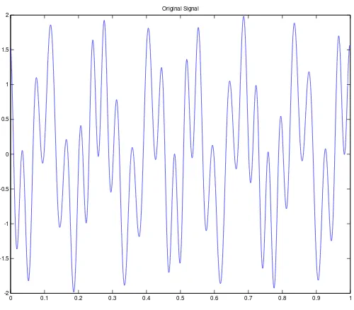
2.1 The Original Signal: The horizontal axis is the time variable and the vertical
axis shows the signal itself. 33
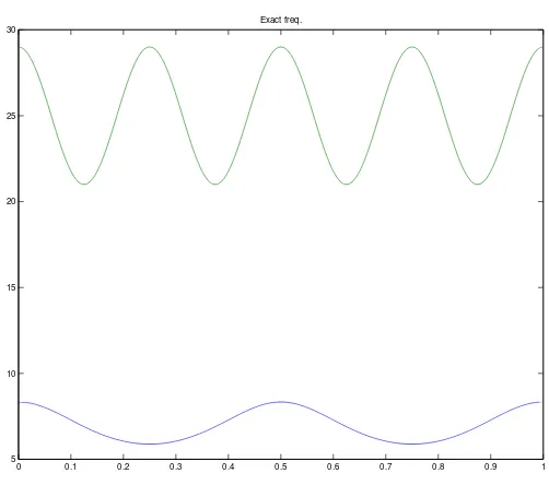
2.2 The Instantaneous Frequencies of the Signal Shown in Figure (2.1): The horizontal axis is the time variable and the vertical axis shows two different
IFs of the constituent IMFs of the signal. 34
2.3 First IMF Extraction: The horizontal axis is the time variable. The extracted IMF is in red and the original IMF is in blue. The extraction is
almost with no error. 34
2.4 First IMF IF: The horizontal axis is the time variable. The extracted IF of the first IMF is in red. It completely overlaps the lowest IF content of the
signal. 35
2.5 Second IMF Extraction: The horizontal axis is the time variable. The extracted IMF is in red and the original IMF is in blue. The extraction is
2.6 Second IMF IF: The horizontal axis is the time variable. The extracted IF of the second IMF is in red. It completely overlaps the highest IF content of
the signal except near the boundaries. 36
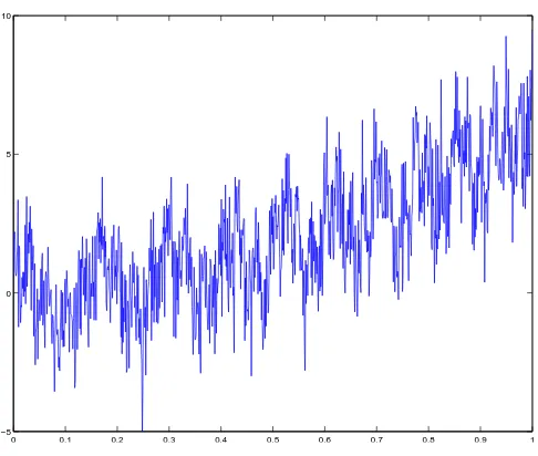
2.7 Original Noisy Signal: The horizontal axis is the time variable and the
vertical axis shows the signal itself. 36
2.8 First IMF Extraction: The horizontal axis is the time variable. The extracted IMF is in red and the original IMF is in blue. The extraction has
some minor error. 37
2.9 First IMF IF: The horizontal axis is the time variable. The extracted IF of the first IMF is in red. It does not overlap the original IF of the signal.
However, it is capturing its trend properly. 37
2.10 Second IMF Extraction: The horizontal axis is the time variable. The extracted IMF is in red and the original IMF is in blue. The extraction is
acceptable even in the presence of noise. 38
2.11 Second IMF IF: The horizontal axis is the time variable. The extracted IF of the second IMF is in red. It does not completely cover the whole trend of the IF due to the presence of noise perturbation. 38
3.1 Signal with a Linear Trend: The horizontal axis is the time variable and the
vertical one is the signal itself. 45
3.2 Extracted Trend: The linear trend is in blue and the extracted trend is in red. Except the right boundary, the error is small in the extracted trend. 45 3.3 Extraction of the first IMF: The extracted IMF is in red. As can be seen,
except from the boundaries the extraction is faithful. 46 3.4 Extraction of the second IMF: The extracted second IMF is in red. It is
almost indistinguishable from the high-frequency original IMF. 46 3.5 Signal with a Quadratic Trend: The horizontal axis is the time variable and
3.6 Extracted Trend: The quadratic trend is in blue and the extracted trend is in red. There is almost no error in the extraction. 47 3.7 Extraction of the first IMF: The extracted IMF is in red. As can be seen,
except from the boundaries the extraction is faithful. 48 3.8 Extraction of the second IMF: The extracted IMF is in red. Like the
previous example, the extraction is accurate, except near the right boundary. 48 3.9 Signal with a Hump-like Trend: The horizontal axis is the time variable and
the vertical one is the signal itself. 49
3.10 Extracted Trend: The trend is in blue and the extracted trend is in red. There is almost no error in the extraction, except near the boundaries. 50 3.11 Extraction of the IMF: The extracted IMF is in red. Since the signal has
intrawave modulation, the extraction has slight phase lags seen near the
peaks and troughs. Still, the extraction is faithful. 50 3.12 Signal with Noise Perturbation: The horizontal axis is the time variable and
the vertical one is the signal itself. 51
3.13 Extraction of the IMF: The extracted IMF is in red. Even in the presence of noise perturbation, the generality of the extraction is acceptable. 51 3.14 Signal with a Quadratic Trend Polluted with Noise Perturbation: The
horizontal axis is the time variable and the vertical one is the signal itself. 52 3.15 Extracted Trend: The linear trend is in blue and the extracted trend is
in red. Due to the presence of noise, the extracted trend deviates from the
original trend slightly. 53
3.16 Extraction of the first IMF: The extracted IMF is in red. The only part of the extraction that is not completely acceptable is the right boundary of the
3.17 Extraction of the second IMF: The extracted IMF is in red. Here, the noise perturbation has more effect on the IMF extraction. However, the generality
of the extraction is still acceptable. 54
4.1 Mild Intrawave Signal vs Narrow Band Filter 61
4.2 Mild Intrawave Signal vs Wide Band Filter 61
4.3 Intrawave Part of the Mixed Signal 62
4.4 High Frequency Part of the Mixed Signal 62
4.5 Intense Intrawave Extraction Failure 64
4.6 Intense Intrawave Extraction 64
4.7 Synchrosqueezed Wavelet Comparison. Top: The frequency spectrum shows that the Synchrosqueezed method detects two major frequency trends. Bottom: The first IMF extracted using this analysis is like the first dominant harmonics. In this analysis, Morlet wavelet was used. 65
4.8 Intense Intrawave with Non-Constant Envelope 65
4.9 EMD Extraction Result for Intrawave Signal with Moving Envelope 66
4.10 Original Signal 66
4.11 Extraction Result of the Mildly Noisy Signal 67
4.12 Original Signal 67
4.13 Extraction Result of the Intensely Noisy Signal 68 4.14 IF: The horizontal axis is the time variable and the vertical axis shows the
IF. 70
4.15 Results of the Extraction 70
4.16 Results 72
4.17 IF of a rare event and an intrawave signal. 73
4.19 Spectrum 74 4.20 Results of the extraction. The red curves correspond to the extracted IMFs. 74
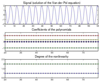
6.1 Top: The solution of the Van der Pol equation; Middle: Coefficients (qk, pk) recovered by our method, star points ∗ represent the numerical results, black
line is the exact one; Bottom: Nonlinearity of the signal according to the recovered coefficients, star points ∗represent the numerical results, black line
is the exact one. 130
6.2 Top: The solution of the Van der Pol equation with noise 0.1X(t), where X(t) is the white noise with standard derivation σ2 = 1; Middle: Coefficients (qk, pk) recovered by our method, star points∗represent the numerical results, black line is the exact one; Bottom: Nonlinearity of the signal according to the recovered coefficients, star points ∗ represent the numerical results, black
line is the exact one. 130
6.3 Top: The solution of the Duffing equation; Middle: Coefficients (qk, pk) recovered by our method, star points ∗ represent the numerical results, black
line is the exact one; Bottom: Nonlinearity of the signal according to the recovered coefficients, star points ∗represent the numerical results, black line
is the exact one. 131
6.4 Top: The solution of the Duffing equation with noise 0.1X(t), whereX(t) is
the white noise with standard derivation σ2 = 1; Middle: Coefficients (q k, pk) recovered by our method, star points ∗ represent the numerical results, black
line is the exact one; Bottom: Nonlinearity of the signal according to the recovered coefficients, star points ∗represent the numerical results, black line
is the exact one. 131
the recovered coefficients, star points ∗ represent the numerical results, black
line is the exact one. 133
6.6 Top: The solution of the equation given in (6.3.1) with noise 0.1X(t),
where X(t) is the white noise with standard derivation σ2 = 1; Middle: Coefficients (qk, pk) recovered by our method, star points ∗ represent the numerical results, black line is the exact one; Bottom: Nonlinearity of the signal according to the recovered coefficients, star points ∗ represent the
numerical results, black line is the exact one. 133 6.7 Top: The solution of the equation given in (6.3.2); Middle: Coefficients
(qk, pk) recovered by our method, star points∗represent the numerical results, black line is the exact one; Bottom: Nonlinearity of the signal according to the recovered coefficients, star points ∗ represent the numerical results, black
line is the exact one. 135
6.8 Top: The solution of the equation given in (6.3.2) with noise 0.1X(t),
where X(t) is the white noise with standard derivation σ2 = 1; Middle:
Coefficients (qk, pk) recovered by our method, star points ∗ represent the numerical results, black line is the exact one; Bottom: Nonlinearity of the signal according to the recovered coefficients, star points ∗ represent the
numerical results, black line is the exact one. 135 6.9 Top: The solution of the equation given in (6.3.2); Middle: Coefficients
(qk, pk) recovered by our method together with the trick in ENO method, star points ∗ represent the numerical results, black line is the exact one; Bottom:
Nonlinearity of the signal according to the recovered coefficients, star points
∗ represent the numerical results, black line is the exact one. 136
6.10 Top: The solution of the equation given in (6.3.2) with noise 0.1X(t), where X(t) is the white noise with standard derivation σ2 = 1; Middle: Coefficients
points ∗ represent the numerical results, black line is the exact one; Bottom:
Nonlinearity of the signal according to the recovered coefficients, star points
∗ represent the numerical results, black line is the exact one. 136
6.11 Top: The signal consists of the solution of the Van der Pol equation and a cosine function and a linear trend and noise 0.1X; Middle: The IMF extracted
from the signal corresponding to the solution of the Van der Pol equation, blue: numerical result; red: exact solution; Bottom: The IMF extracted from the signal corresponding to the cosine function, blue: numerical result; red:
exact solution. 137
6.12 Top: Coefficients (qk, pk) recovered by our method for the first IMF in Fig. 6.11, star points∗ represent the numerical results, black line is the exact one;
Bottom: Nonlinearity of the signal according to the recovered coefficients, star points ∗ represent the numerical results, black line is the exact one. 137
6.13 Top: Coefficients (qk, pk) recovered by our method for the second IMF in Fig. 6.11, star points ∗ represent the numerical results, black line is the
exact one; Bottom: Nonlinearity of the signal according to the recovered coefficients, star points ∗ represent the numerical results, black line is the
exact one. 138
7.1 Instantaneous frequency of the first IMF. The range of instantaneous frequency oscillation (gray band) changes after the dicrotic notch (marked by the red line). a) Instantaneous frequency (top) of the aortic input pressure (bottom) for an aorta with rigidity E1 at HR=100 bpm. b) Instantaneous frequency (top) of the aortic input pressure (bottom) for an aorta with rigidity E1 at HR=70 bpm. c) Instantaneous frequency (top) of the aortic input pressure (bottom) for an aorta with rigidity E3 at HR=70 bpm (E3 =
7.2 Intrinsic frequencies Vs. HR (top graphs) with the corresponding pulsatile power vs. HR (bottom graphs). ω1 (red) is the InF for coupled heart+aorta and ω2 (blue) is the InF for the decoupled aorta. a) Aortic rigidity is E1, the gray band shows that the two IF curves cross each other at the optimum HR (≈110 bpm). b) Aortic rigidity is E2, the two InF curves cross each other at
the optimum HR (≈120 bpm). c) Aortic rigidity is E3, two InF curves cross
each other at the optimum HR (≈140 bpm). 141
7.3 Synthetic Data, with no Noise and Well-Resolved Domain 151 7.4 Synthetic Data, with no Noise and not Well-Resolved Domain 152
7.5 Original Noisy Data 153
7.6 Extracted Curve vs the Original Curve in a Noisy environment 153
7.7 Synthetic trend plus IMF and Noise 154
7.8 Extracted trend for the IMF-Noise case 154
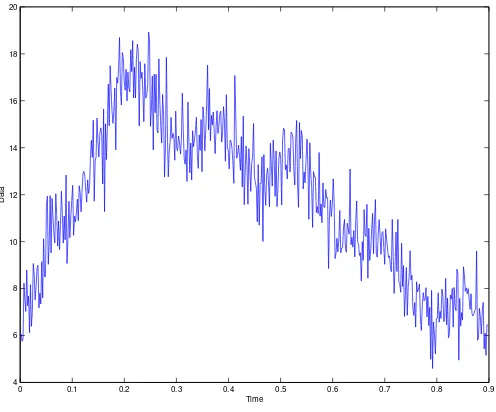
7.9 Recorded Data From iPhone: The data is recorded using iPhone camera. 155
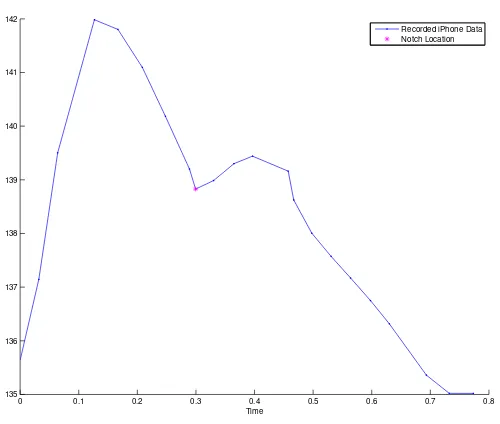
7.10 Extracted IMF from the Recorded iPhone Data 156
7.11 EF Comparison: The vertical axis shows the EF found by 2D
echocardiography. The horizontal axis shows the EF calculated by the InF algorithm. The two dotted green lines show ±15% error offset from the
expected 45 Degree line. 157
8.1 C∞ Compact Support Mollifier 167
List of Tables
3.1 Comparison of the STFR Methods 54
CHAPTER 1
Introduction
1.1. Preamble
Accessing and utilizing the information hidden in such signals requires methods for processing and analyzing signals. Such methods must be able to denoise and analyze the signal in order to properly process the data. Mathematically, the easiest way to construct a signal processing method is to project the recorded signal on a predetermined algebraic basis or dictionary. A classical method of doing this task is the Fourier Transform (FT) method and a more recent one is the Wavelet Transform (WT) method [5, 41].
When a signal is periodic, the FT method is a powerful signal processing method. Using the FT method, one can project the data into the orthonormal basis of the Fourier domain (the frequency domain). This transition is a shift from the time do-main to the frequency dodo-main. The FT method can also perform as a robust method for denoising periodic signals. Fast and efficient implementation of FT, namely the Fast Fourier Transform (FFT) method, is popular among scientists and engineers. The shortcomings of the FT method can be categorized into two different groups. The first is the assumption of the periodicity (or stationarity) of the signal.
method that incorporates a time-frequency analysis of the signal by constructing a large dictionary of some orthonormal functions.
The FT and WT methods share one common property: decomposition is per-formed on a predefined basis, which is troublesome if the signal is not stationary. Recently, Norden Huang proposed Empirical Mode Decomposition (EMD), a new method of adaptive signal processing [30, 32, 33] in which the basis of the projection is adaptive. EMD which uses multiscale data-driven decompositions called Intrinsic Mode Functions (IMFs), is a step forward in data analysis. It has eliminated most of the issues present in the FT and WT methods.
In particular, EMD can produce a faithful extraction even if the signal is not periodic, and makes a sparser time-frequency analysis of the data. In fact, projection into a basis is not the ultimate goal in many recently developed signal processing methods. Researchers wish to have a projection that is as sparse as possible. In other words, it is important to have a representation of the signal in a basis by keeping only a few coefficients containing the pertinent information. In fact, in these methods, one should project the observed signal on a large overdetermined basis (dictionary [10, 12, 42]).
Since the IMFs are extracted adaptively from the data in EMD, the final decompo-sition is in general sparser than FT or WT method the extractions. If the data has a certain frequency scale-separation property, the extracted IMFs convey certain phys-ical properties of the signal. Unfortunately, the empirphys-ical nature of the the EMD’s decomposition makes it hard to analyze the results rigorously. In order to eliminate this problem, Hou and Shi have proposed a rigorous mathematical system as a coun-terpart of the EMD method [25, 24, 26]: the Sparse Time-Frequency Representation (STFR) method.
1.1.1. Scope of the Thesis. The main focus of this thesis is to further develop
STFR method that can analyze non-periodic signals and can robustly deal with sig-nals polluted with noise. Second, we propose and prove the convergence of a new STFR method that can easily analyze intrawave signals, signals with intense Fre-quency Modulation (FM) that cannot currently be handled using Hou and Shi’s STFR methods [25, 24, 26].
Technically speaking, this analysis can be done by relaxing the definition of the dictionaries that Hou and Shi have already used, see (1.2.3). To the best of our knowledge, this is the first time that intrawave signals can be extracted with high accuracy by an adaptive method.
This thesis also presents some real physical applications of our methods. We show that our methods can be applied in diverse fields like dynamical systems and cardiovascular signals. We demonstrate that our method is capable of extracting useful physical and biomedical information from the signals. Such information can possibly be used in system identification and medical diagnosis.
Finally, the thesis also clarifies theoretical understanding of the nature of IMFs. We show that an IMF can have infinitely many representations and that consequently, the uncertainty principle is an indispensable part of oscillating signals. Lacking a unique representation does not decrease the merit of any adaptive data analysis method, including the STFR method, but only shows the richness of the field and requires that an adaptive method can pick a certain representation based on a fixed preference.
1.2. A Brief Introduction to the STFR Method and its Applications
All STFR methods are based on the assumption that a relatively big subclass of the oscillatory signals are signals of the form
with only one extrema between the zeros of the signal, in which the envelope is strictly positive,a(t)>0, and the phase functionθ(t) is a one-to-one, strictly increasing map
between the time coordinate, t, and the phase coordinate, θ. The time derivative of
this phase function is called the Instantaneous Frequency (IF). With some abuse of notation, we can say that the STFR methods deal with signals that have both Amplitude Modulation (AM) and Frequency Modulation (FM). The type of signal, in Equation (1.2.1) is called an Intrinsic Mode Function (IMF) in STFR and EMD terminology. A number of methods can extract each IMF from a combination of many IMFs, with different levels of accuracy. Methods that perform such extraction well include, but are not limited to, EMD [32], EEMD [56], Optimization based EMD [27], Wavelet [41], STFR [25, 24, 26], and Synchrosqueezed wavelet transforms [17]. However, when it comes to signals with strong frequency modulation, these methods have difficulties extracting a unique IMF specifically when the data is polluted with noise. Among these methods, the STFR method provides a better physical and mathematical understanding.
Physically speaking, θ(t) carries information about the rate of the change of the
signal in time. The envelope of each IMF is set to be from a certain collection of functions. In mathematical terms we can express it as
(1.2.2) a(t)∈V (θ(t)) s.t. a(t)>0,
where
(1.2.3) V (θ) = span (
1,cos θ λ
!
,sin θ λ
!
|λ >2 )
.
A finite linear combination of a collection of the IMFs is called an Intrinsic Signal (IS),
(1.2.4) s(t) =
M
X
i=1
ai(t) cosθi(t).
1.2.1. EMD Method. Most of the non-adaptive time-frequency signal
analy-sis methods are based on the projection of a signal on to a predetermined baanaly-sis or dictionary, such as a Fourier transform (FT) or Wavelet transform (WT). However, since the projection of the signal is on a predefined set of functions, the extraction is not adaptive and, possibly, not sparse. In order to get a better time-frequency resolution, the intuition is to project the signal on an adaptive basis that is found from the signal itself. Empirical Mode Decomposition and the more recent Ensemble Empirical Mode Decomposition were developed to do just that.
Empirical Mode Decomposition (EMD) methods were originally proposed to over-come the problem of predetermined bases which was hampering a proper sparse de-composition in the WT and FT methods. EMD [32] tries to find the basis of decom-position adaptively from the original signal in an empirical way. The EMD method uses Intrinsic Mode Function (IMF) [32] as constructing blocks of signals. An EMD definition of an IMF is:
Definition. An IMF is a function that satisfies the following two conditions:
• The number of extrema and the number of zero crossings are equal or differ at most by one on the whole data set
• The mean value of the envelopes defined by the local maxima and the local minima is zero at any point.
EMD decomposes a signal into an extracted IMF and a residue through a sift-ing process. The extracted IMF is then post-processed to find the Instantaneous Frequency (IF) either through Hilbert Transform (HT) or another sifting process [32, 33]. To summarize, for a signal x(t), the decomposition looks like
x(t) =
n
X
k=1
ck(t) +rn(t),
1.2.2. Ensemble Empirical Mode Decomposition (EEMD) Method. EMD
is highly sensitive to noise. In order to fix this shortcoming, Wu and Huang [56] pro-posed EEMD in 2009. EEMD minimizes noise effects by adding white noise to the signal. While the EMD and EEMD methods have attracted a lot of attention, they lack a theoretical basis. The STFR methods were introduced to fill the empirical gap.
1.2.3. STFR Methods. Although STFR methods were inspired by the EMD
and EEMD methods [32, 56], they make use of techniques from compressive sensing theory [10, 12] and matching pursuit [42]. Compressive Sensing (CS) and Matching Pursuit (MP) methods try to find a sparse reconstruction of an observed signal from a predefined finite large dictionary. STFR, on the other hand tries to find a sparse reconstruction of an observed signal from a predefinedinfinitelarge dictionary. STFR methods use two major steps: they first construct a highly redundant dictionary of all IMFs, namelyD, and then find the sparsest decomposition by solving a non-linear
and non-convex optimization problem (1.2.5)
M inimize M
Subject to: s(t) = PM
i=1ai(t) cosθi(t), ai(t) cosθi(t)∈D, i= 1, ..., M, which is an L0 minimization problem. We explain possible approximations by which one can find a close solution of this problem. Hou and Shi have proposed a number of algorithms for approximating this problem [25, 24, 26] by decomposing the signal into two parts, a meana0 and a modulated oscillatory part, namely the IMF,a1cosθ:
s(t) = a0(t) +a1(t) cosθ(t),
1.2.3.1. Total Variation Method. Hou and Shi [24] proposed theT V3 minimization of the form
(1.2.6) M inimize T V
3(a0) +T V3(a1)
Subject to : s(t) =a0(t) +a1(t) cosθ1(t), θ
0
1(t)>0,
as an approximation to the original problem (1.2.5). This problem is solved in an iterative manner. First, an initial guess on θ1 is set. Then based on that, the value of
a1is approximated and the phaseθ1is again updated. This procedure is repeated until there is no progress in updating the phase function. This approach is an exponential step compared to the EMD and EEMD methods; however, the algorithm is not stable to noise.
1.2.3.2. Periodic Fourier-based Sparse Time-Frequency Method. To address the noise instability problem, Hou and Shi, proposed the Periodic Fourier-based STFR method [25], which performs well on periodic data even in the presence of noise. This method implicitly solves
M inimize ks(t)−a(t) cosθ(t)k22
Subject to: a(t) cosθ(t)∈D
using a Fast Fourier Transformation (FFT) iterative scheme. The Periodic STFR algorithm works in the following way: an initial guess is proposed on the phase functionθ0. In the first step, the whole signal is mapped to the phase function space
and the Fourier transform of the signal is then found in that space. At this step, the possible candidates for the envelope functions are found. Later, the new phase function is updated and the algorithm begins a new iteration.
While this algorithm works well for periodic data, the algorithm does not extract the IMFs properly for non-periodic data.
L1-norm regularized with L2-norm optimization rather than FFT for each iteration.
Nevertheless, it can successfully be applied to non-periodic signals and also to signals polluted with noise.
In the non-periodic STFR algorithm, we assume that the envelopes of the IMFs have a sparse structure in their respective dictionary. This assumption is not far from reality since we are using an infinitely large dictionary when we try to extract IMFs. This assumption can be formulated in the following way:
(1.2.7)
M inimize
a,b,θ δ(ka(λ)k1+kb(λ)k1) +ks(t)− A(t) cosθ(t)k 2 2
Subject to: A(t) = ´2∞a(λ) cosθ(t)λ +b(λ) sinθ(t)λ dλ,
dθ(t) dt >0.
In this formulation, the envelopeA(t) of the IMFA(t) cosθ(t) is assumed to have a
sparse structure that is captured byka(t)k1+kb(t)k1. In this formulation, the
dictio-nary is used explicitly by A(t) = ´2∞a(λ) cosθ(t)λ +b(λ) sin θ(t)λ dλ. The following
example shows the performance of this type of STFR.
Example. We tested the algorithm on a signal with a linear trend and two
con-stant envelope and frequency IMFs,f(t) = 6t+ cos (8πt) + 0.5 cos (40πt) (see Figure
1.1). The algorithm extracted IMFs (see red lines in Figures 1.2-1.4). Besides some tiny boundary misalignment, the extractions were accurate, suggesting that the non-periodic STFR method is accurate away from the boundaries.
When compared with other STFR methods, the only shortcoming of the Non-Periodic STFR method is the speed of the algorithm.
1.2.4. Extraction of Intrawave, Sharp, and Rare Event Signals using
Sparse Time-Frequency Method. In general, intrawave signals are oscillatory
signals that have intense frequency modulation in at least one θ-coordinate. By
0 0.1 0.2 0.3 0.4 0.5 0.6 0.7 0.8 0.9 1 −1
0 1 2 3 4 5 6 7 8
Figure 1.1. Signal with a Linear Trend: The horizontal axis is the time variable and the vertical one is the signal itself.
0 0.1 0.2 0.3 0.4 0.5 0.6 0.7 0.8 0.9 1
−1 0 1 2 3 4 5 6
Found IMF Vs real IMFs
0 0.1 0.2 0.3 0.4 0.5 0.6 0.7 0.8 0.9 1 −2
−1 0 1 2 3 4 5 6
Found IMF Vs real IMFs
Figure 1.3. Extraction of the first IMF: The extracted IMF is in red. As can be seen, except from the boundaries the extraction is faithful.
0 0.1 0.2 0.3 0.4 0.5 0.6 0.7 0.8 0.9 1
−1 0 1 2 3 4 5 6
Found IMF Vs real IMFs
absence of noise. However, neither EMD nor EEMD can extract even one intrawave IMF in the presence of noise. If the frequency modulation becomes even more intense, the resulting signal is called a sharp signal. Analyzing these IMFs has so far been a challenging problem in signal processing. Rare events are IMFs with compact support in the time domain. A rare event is essentially like a spike. Adaptive methods like EMD/EEMD are not able to process such signals with acceptable accuracy.
Since the main difficulty in dealing with intrawave signals comes from their wide band representation in the frequency domain, which cannot be properly analyzed using methods with explicit or implicit narrow band filters, we propose a method that modifies the normal envelope dictionary in an STFR framework in order to extract intrawave signals with high accuracy. This small modification, which is enlarging the STFR filter, allows us to treat intrawave signals without major changes to the original STFR Algorithms. Furthermore, we show that although enlarging the filter requires that the IMF components of the IS must have enough separate time-frequency representations, the method is not problematic when extracting non-separable time-frequency IMFs from a signal provided they are extracted simultaneously.
Not only is the algorithm that we use to extract the IMFs stable, then, it is also stable to noise perturbation. The EMD/EEMD methods fail to extract the two IMFs properly. In fact all other adaptive methods fail to extract one IMF with intrawave frequency modulation in the presence of noise, let alone two IMFs with intrawave characteristics that have mode mixture.
1.2.5. Analysis of Convergence of Sparse Time-Frequency Method. We
prove that for any signal, whether intrawave or not, increasing the filter span reduces extraction error. We show that STFR converges to an IMF that is close to one of the IMF representations, but with an error associated with the width (span) of the filter. We assume that an IS can be represented in the following format:
for f1(t)> 0, dθdt =θ0 > 0 and t ∈[0,1]. We assume that the signal is periodic with mean zero. The main convergence theorem states that:
Theorem. Assume that the instantaneous frequency in equation (1.2.8) isM0-sparse; i.e. θ0 ∈VM0 =span
n
ei2πkt,|k| ≤M
0, k ∈Z
o
. Furthermore, assume that
fˆ0,θ¯(k) ≤
C0
|k|p,
fˆ1,θ¯(k) ≤
C0
|k|p
for C0 > 0 and p≥ 4. If the initial guess satisfies
F(4θ
0)0
1
2πM0 ≤
1
4, then there exists an η0 >0 such that forL > η0 we have
F(θ−θ
m+1)0
1 ≤ Γ1λ
2p−2L−p+2+ 1 2
F(θ−θ
m)0 1
for λ >1 and Γ1 >0. Here, ˆfθ¯(k) =
´1 0 f
¯
θe−i2πkθ¯dθ¯and (F(g)) k =
´1 0 g(t)e
−i2πktdt. This theorem can be generalized to the case where the signal is polluted with noise. Take
(1.2.9) f(t) = f0(t) +f1(t) cosθ(t) +=,
where = is a periodic perturbation to the original signal.
Theorem. Assume that the instantaneous frequency in equation (1.2.9) isM0-sparse; i.e. θ0 ∈VM0. Furthermore, assume that
fˆ0,θ¯(k) ≤
C0
|k|p,
fˆ1,θ¯(k) ≤
C0
|k|p
for C0 > 0 and p≥ 4. If the initial guess satisfies
F(4θ
0)0
1
2πM0 ≤
1
4, then there exists an η0 >0 such that forL > η0, and k=k∞ ≤0 (0 sufficiently small) we have
F(θ−θ
m+1)0
1 ≤ Υ0(L, λ)k=(t)k∞+ Γ1λ
2p−2L−p+2+1 2
F(θ−θ
m)0
These theorems explain only that we have a convergent algorithm, not that the algorithm’s extraction is unique. Uniqueness is a difficult theoretical problem that requires further research for more clarification.
1.2.6. Applications of Sparse Time-Frequency Method. In this thesis, we
study the application of STFR in two different fields: dynamical systems and cardio-vascular disease diagnosis.
1.2.6.1. Dynamical Systems: In many scientific applications that requires signal analysis, such as biological investigations, the complexity of the underlying physi-cal problem is perplexing and the appropriate governing equation that describes its dynamics is unknown. Researchers would like to be able to determine whether the underlying dynamical system is linear or nonlinear, including quantifying the degree of any nonlinearity.
We present a method for quantifying the nonlinearity of IMFs given by the STFR method. The main idea is to establish a connection between the IMFs and classical second order differential equations. We show that each IMF can be associated with a solution of a second order ordinary differential equation of the form ¨x+p(x, t) ˙x+ q(x, t) = f(t). This method provides a new way to interpret the hidden intrinsic
information contained in the extracted IMF of a signal.
1.2.6.2. Cardiovascular Disease Diagnosis: Cardiovascular Diseases (CVD) are one of the main causes of death in the United States every year [39]. With an in-creasing number of deaths every year, there is a need to develop new CVD diagnosis methods.
It is assumed that before and after the dicrotic notch, we have the following simple waveforms for the general IMF of the aortic pressure wave at time t:
si =aicosωit+bisinωit+ ¯p, i= 1,2.
This assumption has shown its credibility as an index to characterize the heart and cardiovascular diseases [44]. In this formula, i = 1 corresponds to the behavior of
the IMF before the valve closure, and i = 2 to the behavior of the IMF after that.
Here, ai, bi are constants and correspond to the envelopes of the IMF. The constants
ω1, ω2 correspond to the InFs of the IMF. ¯pis the mean pressure during the heartbeat period.
Take [0, T] to be the whole period of the pressure wave and T0 as the location of the dicrotic notch: 0< T0 < T. Also, define the indicator function as
1[x,y)(t) =
1, x≤t < y,
0, else.
Now, the main IMF of the pressure waveform can be expressed as
S(ai, bi,p, ω¯ i;t) = (a1cosω1t+b1sinω1t+ ¯p)1[0,T0)(t) +
(a2cosω2t+b2sinω2t+ ¯p)1[T0,T)(t).
The goal is to extract the IMF carrying most of the energy and consequently the InFs, ω1, ω2, from the observed aortic pressure waveform f(t). Taking t as a continuous variable, one can use the least squares minimization to find the unknowns.
minimize
ai,bi,ωi,¯p
kf(t)−S(ai, bi,p, ω¯ i;t)k 2 2
subject to a1cosω1T0+b1sinω1T0 = a2cosω2T0+b2sinω2T0, a1 = a2cosω2T +b2sinω2T.
We employed the InF algorithm on pressure wave signals collected from human beings (both invasively using a catheter and non-invasively using an iPhone camera) and dogs (invasively using a catheter). We found that heart performance (the Ejection Fraction1 (EF)) can be predicted using the normalized values of the InFs and the normalized value of ¯p. The performance of the InF algorithm clearly shows potential
for use in health care systems.
1Ejection Fraction is essentially a measure of the percentage of blood leaving the heart in each
CHAPTER 2
Literature Review
While there are different methods for signal processing, this chapter provides an introductory overview of the more prevalent methods of signal decomposition and processing, focusing on Fourier methods, Wavelet methods, and Empirical Mode Decomposition methods, as well as a brief review of the Total Variation (TV) STFR method[24], a first generation STFR method. Further details on these topics can be found in the references cited in this chapter. This overview follows the steps of the work by Guignard [23].
2.1. Fourier Methods
The classical approach to signal decomposition, Fourier analysis or Fourier Trans-form, was first proposed by French mathematician Joseph Fourier, who initially used it to solve heat transfer problems [7]. The most famous because of its simplicity and accuracy, Fourier analysis decomposes a signal over a frequency space. Here, we briefly introduce the method in mathematical terms.
2.1.1. Fourier Series.
Definition 1. Take the 2π-periodic real function f ∈ L1(0,2π), and N ∈
N. The
Partial Fourier Series of order N of the function f is defined by
(2.1.1) FN(f(t)) = a0+ N
X
n=1
(ancos (nt) +bnsin (nt)),
having
a0 = 1 2π
ˆ 2π
0
f(t)dt,
an= 1
π
ˆ 2π
0
bn= 1
π
ˆ 2π
0
f(t) sin (nt)dt.
This real definition can be extended into the complex form.
(2.1.2) FN(f(t)) =
N
X
n=−N
cneint,
with
(2.1.3) cn=
1 2π
ˆ 2π
0
f(t)e−intdt.
The Fourier Series of a function, if exists, is defined as
F(f(t)) = lim
N→∞FN (f(t)).
In order to extend the Fourier Series from L1(0,2π) functions into L2(0,2π), we first
need to show that the set
(2.1.4)
(
1
√
2π,
cos (mt)
√
π ,
sin (nt)
√
π )
,
is an orthonormal set for m, n∈N. This can be shown using the relations
ˆ 2π
0
cos (mt) sin (nt)dt= 0,
ˆ 2π
0
sin (mt) sin (nt)dt=
π, m=n
0, m6=n ,
and
ˆ 2π
0
cos (mt) cos (nt)dt=
π, m=n
0, m6=n .
The following theorem shows that the set (2.1.4) is an orthonormal basis forL2(0,2π)
[5].
Theorem 1. Let f ∈L2(0,2π). Then
lim
where kFN(f(t))−f(t)k2 =
´2π
0 |FN(f(t))−f(t)| 2
dt
1 2
. Furthermore, the Par-seval’s identity is satisfied
ˆ 2π
0
|f(t)|2dt= 2π
N
X
n=−N
|cn| 2
.
2.1.2. Fourier Transform (FT). The Fourier transform is the continuous
ver-sion of the Fourier Series. Here the function is not necessarily periodic and it is defined on the whole real axis.
Definition 2. Let f ∈L1(R). Then, the Fourier Transform of f is defined as
F(k) = √1
2π
ˆ ∞
−∞
f(t)e−iktdt.
If F ∈L1(
R), the function f can be recovered by
f(t) = √1
2π
ˆ ∞
−∞
F(k)eiktdk.
To properly define the Fourier Transform if f ∈ L2(
R), but is not in L1(R), one
must find a sequence of functions fN ∈L1(R)∩L2(R) which converges to f in the
L2 sense. Then the above definition can be used for fN as N goes to infinity.
2.1.3. Fast Fourier Transform (FFT). In practice, the recorded signal is
al-ways in a discrete format, f = (f0, . . . , fN−1)T. Without loss of generality, one can
assume that the data is recorded on a uniform mesh, tn = 2πnN , forn = 0, . . . , N −1. Using the trapezoidal rule, one can evaluate (2.1.3) to find the Fourier Series F =
(F0, . . . , FN−1)T in a discrete way:
Fk = N−1
X
n=0
fne−
i2πkn
N ,
for k = 0, . . . , N −1. The original signal can be recovered using
fn= 1
N
N−1
X
k=0
Fke
i2πkn
Now, the discrete Fourier transform can be be written in a matrix multiplication form. Take the following Vandermonde matrix by lettingω =e2Nπi.
M=
1 1 1 · · · 1
1 ω ω2 · · · ωN−1
1 ω2 ω4 · · · ω2(N−1)
... ... ... ... ... 1 ωN−1 ω2(N−1) · · · ω(N−1)2
Hence, F =Mf. This matrix multiplication needs O(N2) operations. However, by rearranging the terms in odd and even members in f, the algorithm can speed up to O(NlogN) [15]. The latter is called the FFT method. In fact, the FFT method is
a descendant of the divide and conquer algorithms.
2.1.4. Windowed Fourier Transform (WFT). Since Fourier Series suffers
from the fact that there is no information about temporal instances in the Fourier domain, WFT was proposed by Gabor [41]. WFT analyzes a small part of the signal by multiplying it by a window function that is real, symmetric and non-zero:
Fg(k, s) = √1 2π
ˆ ∞
−∞
f(t)g(t−s)e−iktdt.
whereg is the window function. While this provides information regarding the
time-frequency nature of the signal, it does not completely find the time-time-frequency con-tent of the signal. Depending on the length of the support of the window function, one can get different time-frequency resolutions due to the Heisenberg Uncertainty Principle. Furthermore, it is almost impossible to distinguish between the different time-frequency contents of the different components of a signal that is made up of many AM-FM signals.
2.1.5. Heisenberg Uncertainty Principle. A time signal f and its Fourier
transform F cannot be simultaneously localized in a small domain of the time and
including the WFT, can exactly state whether a certain frequency has happened at a certain time.
To enable better time-frequency resolution, the Wavelet Transform (WT) was introduced [16]. WT does not defy the Heisenberg Uncertainty Principle; however, it tries to present a decomposition that eliminates the principle’s side effects as much as possible.
2.2. Wavelet Methods
Wavelet Transform was introduced to analyze a signal at different scales more accurately than WFT [16]. WT extracts the details of a signal at different time and frequency scales.
2.2.1. The Wavelet Transform. A wavelet is a complex function ψ : R → C
satisfying the following conditions: (1) ψ ∈L2(
R)
(2) Cψ := 2π
´
R∗
|F(ψ)(a)|2
|a| da <∞,
whereF(ψ) is the FT of ψ, andR∗ =R− {0}. A wavelet dictionaryDis the dilation
and translations of the wavelet ψ:
(2.2.1) D={ψa,b(t),(a, b)∈R∗ ×R},
where ψa,b(t) = |a|
−1
2 ψt−b
a
. The parameters a, b are the scaling and translational
parameters respectively. The wavelet transform of a signal is defined as the inner product of the signal f and the wavelet function:
(2.2.2) Wf(a, b) := hf, ψa,bi=|a|
−1 2
ˆ ∞
−∞
f(t)ψ t−b a
! dt.
One can recover the original function from the transform by
(2.2.3) f = 1
Cψ
ˆ
R∗×R
The parameter b is a translational parameter that can spot the occurrence, in the
time domain of a certain frequency, which is characterized by the scaling parameter
a. Hence, the wavelet transform Wf(a, b) conveys the information regarding the
time-frequency content of a signal. Numerical approximation of Wavelet Analysis is called Multiresolution Approximations.
2.2.2. Multiresolution Approximations. A fast and numerically feasible
ap-proximation of a signal at different scales requires an orthonormal basis of L2(R) at
different scales, in other words, an orthogonal projection on {Vj}j∈Z, as defined in Definition 3, so that the behavior of the signal at different scales can be captured. Here we present the properties of multiresolution spaces [41]:
Definition 3. The sequence of closed subspaces of L2(
R), namely {Vj}j∈Z, is a multiresolution approximation, if the following properties are satisfied:
1- Translation Invariance: f(t)∈Vj ⇔f(t−2jn)∈Vj for all (j, n)∈Z2. 2- Nesting: Vj+1 ⊂Vj for all j ∈Z.
3- Scaling: f(t)∈Vj ⇔f
t
2
∈Vj+1 for all j ∈Z. 4- Separation: ∞T
j=−∞Vj ={
0}.
5- Density: ∞S
j=−∞
Vj =L2(R).
6- Existence of Riesz Basis: There existsθsuch that{θ(t−n)}n∈
Zis a Riesz basis
of V0.
Using this definition, the following theorem constructs a family of orthonormal basis for Vj [41].
Theorem 2. Let {Vj}j∈Z be a multiresolution approximation and φ be the scaling function satisfying
F(φ) (ξ) = F(θ) (ξ)
P∞
k=−∞|F(θ) (ξ+ 2kπ)|
Then the family {φj,n}n∈Z is an orthonormal basis of {Vj}j∈Z. Here, φj,n is defined as
φj,n = 1
√
2jφ
t−2jn 2j
! .
To find the orthonormal basis of L2(R), one must first find the orthogonal
com-plement of Vj, namelyWj, in Vj−1,
Vj−1 =Vj ⊕Wj.
This can be achieved using Theorems 3 and 4 [5, 41].
Theorem 3. Let φ be a scaling function and let ψ be the function that satisfies
F(ψ) (ξ) =eiξ2H ξ
2+π
!
F(φ) (ξ).
HereH(ξ) = √1
2
P∞
n=−∞hne−inξ, withhn =hφ(t), φ−1,n(t)i. Then the family{ψj,n}n∈Z
is an orthonormal basis of {Wj}j∈Z, with
ψj,n = √1 2jψ
t−2jn 2j
! .
Theorem 4. The family{ψj,n}(j,n)∈Z2 , is an orthonormal basis of L2(R).
These theorems enabled the development of the Fast Wavelet Transform (FWT) algorithm. The FWT algorithm decomposes an approximationfj ∈Vj into a coarser approximation fj+1 ∈ Vj+1 and the details wj+1 ∈ Wj+1 and is then applied to
fj+1 ∈Vj+1. In other words, for a K−1 step algorithm we have
fj =fj+K+ j+K
X
k=j+1
wk.
For further details of the algorithm, see [41].
the extraction is not adaptive. In order to get a better time-frequency resolution, the intuition is to project the signal on an adaptive basis that is found from the signal itself. Empirical Mode Decomposition and the more recent Ensemble Empirical Mode Decomposition were developed to do just that.
2.3. Empirical Mode Decomposition (EMD) Methods
Empirical Mode Decomposition (EMD) methods were originally proposed to over-come the problem of predetermined bases which was hampering a proper sparse de-composition in the WT and FT methods. EMD [32], which tries to find the basis of decomposition adaptively from the original signal in an empirical way, has gained much acceptance in the engineering and scientific community [30, 31].
2.3.1. EMD Algorithm. The EMD method uses Intrinsic Mode Function (IMF)
[32] as constructing blocks of signals. IMFs are defined slightly differently in different methods. Here, we present an EMD definition of an IMF.
Definition 4. An IMF is a function that satisfies the following two conditions:
• The number of extrema and the number of zero crossings are equal or differ at most by one on the whole data set
• The mean value of the envelopes defined by the local maxima and the local minima is zero at any point.
EMD decomposes a signal into an extracted IMF and a residue through a sifting process. The extracted IMF is then post-processed to find the Instantaneous Fre-quency (IF) either through Hilbert transform or another sifting process [32, 33]. To summarize, for a signal x(t), the decomposition looks like
x(t) =
n
X
k=1
ck(t) +rn(t),
Algorithm 1EMD Sifting Algorithm
• 1: k = 1
• 2: Find all local extrema ofx(t)
• 3: Interpolate the minima (using cubic spline) to get the lower envelope
emin(t)
• 4: Interpolate the maxima (using cubic spline) to get the upper envelope
emax(t)
• 5: Compute the meanm(t) = emax(t)+emin(t)
2
• 6: Extract the detaildk(t) = x(t)−m(t)
• 7: ifdk(t) satisfies the definition of an IMF then
• 8: return c(t) = dk(t)
• 9: else
• 10: x(t) =dk(t)
• 11: k =k+ 1
• 12: go to 2. • 13: end if
decreasing, or has only one local minimum or maximum. The original EMD sifting algorithm, which is explained in Algorithm 1 [23], extracts only one IMF from the signal. Hence, when one IMFc(t) is extracted from the signalx(t), then x(t)−c(t)
is considered to be a new signal (if it is not already a residual) and the sifting process is now performed on this new signal. This procedure is done repeatedly until all IMFs are extracted.
There is a problem with the sifting algorithm: the sifting process can inadvertently eliminate physical information about the extractions by over-smoothing. In order to prevent such an error, a stopping criterion is needed [32]. Taking a parameter like
SD =
N
X
i=1
|dk(ti)−dk+1(ti)|2 (dk(ti))2
,
it is possible to define an empirical stopping criterion. Here, it is assumed that the signal is sampled on discrete points ti, i= 1, . . . , N. Usually, if SD is less than 0.2 or 0.3, the sifting process must stop. Unfortunately, this is another empirical nature of
the algorithm.
residue. The extractions finally stop when the residual is too small or it is monotonic. Once all the IMFs are extracted, the IF can be found by the Hilbert transform or another sifting process on the IMF [33]:
First, the Hilbert transform of the j-th IMF cj is defined as
hj(t) = 1
π
∞
−∞
cj(τ)
t−τdτ.
Next, the analytic signal of the Hilbert transform is defined as
zj(t) = cj(t) +ihj(t) = aj(t)eiθj(t).
At the end, the IF is defined as the time derivative of θj(t). In other words, ωj(t) = dθj(t)
dt . The problem with this approach is that the found IF is based on a certain definition that is derived from an analytic signal.
2.3.2. Ensemble Empirical Mode Decomposition (EEMD) Algorithm.
EMD is highly sensitive to noise. In order to fix this shortcoming, Wu and Huang [56] proposed EEMD in 2009. EEMD minimizes noise effects by adding white noise to the signal. The method then follows with finding the IMF, repeating the same procedure with many other realizations of the white noise, and finally take the average of these IMFs as the corresponding IMF. The number of times that the white noise is added is called the ensemble number E. The EEMD algorithm is detailed in Algorithm 2,
[23].
The total number of IMF extractions should remain the same throughout each time that the noise is added to the signalxi(t), which is a shortcoming of the EEMD. The proposed number is usuallyblog2Nc−1 for a signal of lengthN [56]. This is again
Algorithm 2EEMD Algorithm
• 1: for i= 17−→E do
• 2: Let wi(t) be a white noise series
• 3: Computexi(t) = x(t) +wi(t)
• 4: Perform the decomposition of xi(t) using the EMD method:
xi(t) = n
X
j=1
cj,i(t) +rn,i(t),
• 5: end for
• 6: Compute the (ensemble) mean IMFs
cj(t) = 1
E
E
X
i=1
cj,i(t), forj = 1, . . . , n.
2.4. STFR Methods
Although STFR methods were inspired by the EMD and EEMD methods [32, 56], they make use of techniques from compressive sensing theory [10, 12] and matching pursuit [42]. Compressive Sensing (CS) and Matching Pursuit (MP) methods try to find a sparse reconstruction of an observed signal from a predefined finite large dic-tionary. STFR, on the other hand tries to find a sparse reconstruction of an observed signal from a predefined infinite large dictionary. STFR methods use two major steps: they first construct a highly redundant dictionary of all IMFs, namely D, then
find the sparsest decomposition by solving a non-linear and non-convex optimization problem (2.4.2), an L0 minimization problem. Solving it is fundamentally difficult. In the coming parts, we explain possible approximations by which one can find a close solution of problem (2.4.2).
In order to explain the STFR methods, we need some preliminary definitions. The set of the collection of IMFs constitute a dictionary. However, before defining the dictionary of IMFs, we need another definition.
Definition 5. The envelope functions set V (θ) is
V (θ) = span (
1,cosθ λ,sin
θ
λ |λ≥λ0 )
where λ0 is called the level of smoothness.
A common value for λ0 is 2 so that the frequencies of the envelope terms are always less than or equal to 1
2, in θ-coordinate. This states that the envelope is not as oscillatory as cosθ.
Definition 6. The IMF dictionary D is defined as
(2.4.1) D= (
a(t) cosθ(t)|a(t)∈V (θ(t)), a(t)>0,dθ(t) dt >0,
dθ(t)
dt ∈C
) .
The goal of the STFR methods is to find the sparsest decomposition among all possible IMFs in a dictionary. In mathematical terms, the sparsest decomposition of the signal is to be found by solving a nonlinear optimization problem
(2.4.2)
M inimize M
Subject to: s(t) = PM
i=1ai(t) cosθi(t), ai(t) cosθi(t)∈D, i= 1, ..., M. The assumption behind this optimization problem is that the nature of the signal is nothing but an IS. This problem is an L0 minimization. Like other optimization problems, the constraints(t) =PM
i=1ai(t) cosθi(t) can be relaxed into an inequality inL2-norm if noise (or approximation error) is present in observation.
The optimization problem (2.4.2) is NP hard. Hou and Shi have proposed a number of algorithms for approximating this problem [25, 24, 26] by decomposing the signal into two parts, a mean a0 and a modulated oscillatory part, namely the IMF,
a1cosθ:
s(t) = a0(t) +a1(t) cosθ(t),
a preset value. This part of the STFR methods is essentially the same as the one we observed in the EMD and EEMD methods.
2.4.1. Total Variation (TV) Method. To find a good acceptable
approxima-tion, Hou and Shi [24] proposed an adaptive STFR method based on total variation minimization, the TV STFR method. They used TV to impose a smoothness condi-tion on the meana0(t) and envelopea1(t) functions. It is well known that minimizing the total variationT V (g) =´ab|g0(x)|dx would generate the “stair case.” As a result,
Hou and Shi proposed the T V3 minimization1 of the form
(2.4.3) M inimize T V
3(a0) +T V3(a1)
Subject to : s(t) =a0(t) +a1(t) cosθ1(t), θ
0
1(t)>0,
as an approximation to the original problem (2.4.2). This enforces a higher order regularity of the local median and envelope. Minimizing the third-order total variation of any function tends to produce a piecewise constant approximation to the third order derivative of the function. Thus, aT V3 minimization tends to produce a cubic spline approximation fora0(t) anda1(t). In this sense, this method is similar to that of the EMD method.
This problem is solved in an iterative manner. First, an initial guess on θ1 is set. Then based on that, the value of a1 is approximated and the phase θ1 is again updated. This procedure is repeated until there is no progress in updating the phase function. Here, the definition of the dictionary is not used explicitly. The smooth-ness requirements of the mean a0 and the envelope a1 are enforced through a T V3 minimization. This approach is an exponential step compared to the EMD method and fixed-basis methods like FT and WT methods. Unfortunately, the algorithm is not stable to noise.
1T Vn(g) =´b
a|g
(n+1)(x)|dx=