R E S E A R C H
Open Access
Cubic time algorithms of amalgamating gene
trees and building evolutionary scenarios
Vassily A Lyubetsky
1*, Lev I Rubanov
1, Leonid Y Rusin
1,2and Konstantin Yu Gorbunov
1Abstract
Background:A long recognized problem is the inference of the supertreeSthat amalgamates a given set {Gj} of
treesGj, with leaves in eachGjbeing assigned homologous elements.
We ground on an approach to find the treeSby minimizing the total cost of mappingsαjof individual gene trees
GjintoS. Traditionally, this cost is defined basically as a sum of duplications and gaps in eachαj. The classical
problem is to minimize the total cost, whereSruns over the set of all trees that contain an exhaustive non-redundant set of species from all inputGj.
Results:We suggest a reformulation of the classicalNP-hard problem of building a supertree in terms of the global minimization of the same cost functional but only over species treesSthat consist of clades belonging to a fixed setP(e.g., an exhaustive set of clades in allGj). We developed a deterministic solving algorithm with a low degree
polynomial (typically cubic) time complexity with respect to the size of input data.
We define an extensive set of elementary evolutionary events and suggest an original definition of mappingβof treeGinto treeS. We introduce the cost functionalc(G,S,f) and define the mappingβas the global minimum of this functional with respect to the variablef, in which sense it is a generalization of classical mappingα.
We suggest a reformulation of the classicalNP-hard mapping (reconciliation) problem by introducing time slices into the species treeSand present a cubic time solving algorithm to compute the mappingβ. We introduce two novel definitions of the evolutionary scenario based on mappingβor a random process of gene evolution along a species tree.
Conclusions:Developed algorithms are mathematically proved, which justifies the following statements. The supertree building algorithm finds exactly the global minimum of the total cost if only gene duplications and losses are allowed and the given sets of gene trees satisfies a certain condition. The mapping algorithm finds exactly the minimal mappingβ, the minimal total cost and the evolutionary scenario as a minimum over all possible
distributions of elementary evolutionary events along the edges of treeS.
The algorithms and their effective software implementations provide useful tools in many biological studies. They facilitate processing of voluminous tree data in acceptable time still largely avoiding heuristics. Performance of the tools is tested with artificial and prokaryotic tree data.
Reviewers:This article was reviewed by Prof. Anthony Almudevar, Prof. Alexander Bolshoy (nominated by Prof. Peter Olofsson), and Prof. Marek Kimmel.
Keywords:Phylogenetics, Fast algorithms, Tree inference, Species tree, Tree amalgamation, Tree reconciliation, Supertree, Evolutionary events, Gene duplication, Gene loss, Horizontal gene transfer, Gene gain, Time slices
* Correspondence:[email protected]
1Institute for Information Transmission Problems, The Russian Academy of
Sciences (Kharkevich Institute), Bolshoy Karetny per. 19, Moscow 127994, Russia
Full list of author information is available at the end of the article
Background
Problems in supertree inference
DenoteSa tree of species or other taxonomic units, pro-teins, etc. The long recognized problem is to infer a treeS
that amalgamates a given set {Gj} of treesGj, with leaves
in eachGjbeing assigned homologous sequences from an
j-th family of homologous elements. Only leaf names, not sequences themselves, are considered. Henceforth, assume that leaves inSare labeled with species namesx, leaves in eachGj–with species-gene namesx-y(gene“y”exists in
species “x”); paralogs are allowed. Refer to S as aspecies tree, and to eachGjas agene tree.
We elaborate a traditional approach from [1,2] to find
the tree S such that it minimizes the total cost of
map-pings of individual gene treesGjintoS.
Traditionally, some cost c(G,S) of mapping of a gene
tree G into a species tree S is defined. Choosing a
par-ticular definition of c(G,S) (ref. e.g. to [2,3] and see Results) is not essential in terms of solving the classical
problem below. For a given set {Gj} of gene trees the
total costis defined as
c Gj ;S
¼X
j
c Gj;S
or
c Gj ;S
¼X
j
kj:c Gj;S
ð1Þ
wherekjare certain weights. The classical problemis to
find suchSthat globally minimizes the functionalc({Gj},
S), where S runs over the set of all species trees that
contain an exhaustive non-redundant set of species from all inputGj. SuchSis called asupertreefor the given set
{Gj}. Denote V0 a set of all species names occurring in
leaves of the input trees Gj. Thus, the classical problem
is to find the global minimum of cost functional (1) over all species treesSthat possess the setV0of leaf names.
The supertree building problem is NP-hard, i.e., any
algorithm to solve it must possess an exponential complex-ity (if NP ≠P). Numerous heuristics exist (e.g. in [4-6]), which however do not provide evaluations of the runtime of corresponding algorithms. UnlessNP=P, none of them can possess a polynomial complexity and be proved to find the true global minimum.
We propose a reformulation of the classical problem and develop an effective deterministic algorithm that meets many biological prerequisites (Description of the
first algorithm and Results). Namely, the supertree S is
sought for as a global minimum of (1) butS runs over a
set of such species trees that mostly contain clades present in input trees Gj, [3,7,8]. A set of species names
assigned to leaves of a subtree in Gj with the root vis
called a clade (of vertex v in Gj) and denoted by cl(v).
The set P includes all clades from trees Gj and
additionally the set of species names V0. Such P is
re-ferred to as a standard set. Its cardinality has the order ofnm, wherenis the number of gene trees, andmis the total number of species. For the standard setP, the algo-rithm’s running time is cubic and determined by formula (2) below.
Further, suppose thatcl(v1),cl(v2) are the clades of two
noncomparable verticesv1,v2in a treeGj, and the
inter-section I(v1,v2) of these clades is not empty. Optionally,
the sets cl(vi) – I(v1,v2), (i=1, 2) are also included in P;
and for each vertexvthat is ancestral tovi (i=1 ori=2)
but not to another vertex from the pair v1,v2, the setcl
(v)– cl(vi) is included inP. In so doing, horizontal gene transfers are accounted forin a species tree, ref. to [9].
IfPincludes any other nonempty subsets ofV0and its
cardinality is arbitrary, the algorithm remains cubic in time but with respect to cardinality |P| of set P, ref. to formula (3) below.
Therefore, the non-standard problem formulated in
this study consists of finding the global minimum of functional (1) among species treesSthat have the set of leaves V0 and a set of clades belonging to a fixed setP.
Thus,Pis a parameter of the problem and of the solving
algorithm. The algorithm operates equally with any P.
The solution is also referred to as asupertree or a“ lim-ited supertree”with respect toP.
A mapping of Gj into S, as well as defyning any
sce-nario, requires a pre-defined fixed set of elementary evo-lutionary events. The standard set (of events) contains
only gene duplications and losses. The extended set (of
events) additionally contains horizontal gene transfers, gains, etc. The list of elementary evolutionary events and their definitions are given in Description of the first al-gorithm. Henceforth, edges in a species tree are referred
to as tubes to contrast the difference with the edges in
gene trees.
With the standard event set, the algorithm possesses the running time of
O n m 3ðnþmÞ ð2Þ
For simplicity, here we assume that the average num-ber of leaves in given treesGjis multiple ofm.
If set P has an arbitrary cardinality, the mentioned
time has the order of
O Pj j3þj jP2nmþj jPm3 ð3Þ Let a set {Gj} of gene trees and its associated P be fixed. A setV∈Pis defined asbasicif it is either a single-ton set or can be split into two basic sets. Let us intro-duce the condition
The condition imposes a certain dependency between sets {Gj},PandV0.
With the standard event set and condition (*), the algorithm was mathematically proved [7], which means
that it outputs the true global constrained minimum of
the corresponding functional.
It is difficult, however, to mathematically prove the algorithm for the case of the extended event set and/or a relaxation of condition (*). We believe that including horizontal gene transfers still produces valid results [7], and/or condition (*) can be relaxed.
The authors are unaware from published literature of
analogous approaches to find a mathematically proved
supertree incubic time.
In Testing of the algorithms we present testing of the supertree building algorithm with artificial and biological data.
A relevant biological discussion of our approach is provided in [8]. The mapping cost in [3] is similar to the cost from [2] in the case of standard event set.
Problems in inferring evolutionary scenario
Patterns of gene evolution possess a number of various types of events that co-occur with the species evolution. Identification of these types and assembling elementary events into an evolutionary scenario is crucial for under-standing the evolutionary histories of genes, genomes, species, and higher taxonomic lineages, ref. e.g. to [10-12]. Important is to create a model that incorporates all known event types, as well as a model of co-evolution of regulatory systems, genes and species, e.g. [13]. Studies (e.g. in [14]) show the importance of considering suboptimal (in terms of the total cost) solutions in searches, as those might rep-resent optimal scenarios when the costs of elementary events are slightly varied. This problem is partially tackled in Second scenario design: a random process on the graph.
In pioneer papers [2], thecost c0(G,S) is defined through
themappingα(G,S) of a given treeGintoSbasically as a sum of duplications (pairs <x, z>, where α(x)=α(z)) and gaps (verticesy, where there is noxfor whichy=α(x)). For
the givenGandS, the mappingαcan be computed as a
global minimum of the functional c0(G,S,f) that depends
on the variablefrunning over a suitable set of mappings
fofGintoS; such αcan be obtained in linear time with respect to the size of input data, and c0(G,S) becomes
equal toc0(G,S,α). Definitions of the cost and mapping
are closely related to the definition of the evolutionary scenario, i.e., a pattern of elementary evolutionary events
that a gene undergoes along the branches of tree S. An
important part of this definition is the choice of allowed elementary evolutionary events and their costs. In [2] the list included only gene duplications and losses. We consider the extended set of elementary evolutionary events listed in the Methods, and the novel definition of
cost c(G,S) (see Computing the total cost of binary gene trees against the species tree).
If horizontal gene transfers are allowed, any mapping algorithm suffers from an intrinsic prohibition of gene transfers across different levels of the species tree. If this prohibition holds, the problem of building the globally minimal (i.e., globally minimizing the cost functional) mapping ofGintoSisNP-hard.
In order to circumvent the NP-hard nature of the
problem and develop a polynomial time algorithm to solve it, the concept of time slices in species treeS was introduced [3,15,16]. This concept is in some sense related to an earlier approach to date tree vertices [17]. The concept is biologically justified, although its correct definition is still to be developed.
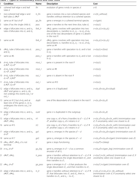
More precisely, edges of S can be broken by inserting
additional vertices, thus formally producing another tree
S0, Figure 1; in the special case S=S0. It imposes time
slices inS such that any horizontal transfers are allowed but only within one slice. The algorithm of building time slices [3,15] constructs the tree S0 such that the k-th
slice contains all edges distant by the amount ofkedges from the root. Naturally, any two consecutive edges in
S0belong to different slices.
Recall that edges inS0andSare referred to astubesto
contrast the difference with the edges in gene trees; inserted vertices split a tube into a succession of new tubes.
The generalization of mapping α is proposed for the
case of the extended set of elementary evolutionary events listed in Description of the first algorithm. This
R R
S R'
d0
S0 R'
d0
d*
1 2 3 d*
1 2 3
Figure 1A transition from treeSto treeS0.Leaves 1, 2, 3 contain in-group species, leafd*contains an auxiliary outgroup species. Leafd*is connected to the root by theoutgroup tube
(shown in bold). All tubes acquire additional vertices during transition toS0(right, shown in bold) to delimit time slices (here four slices are separated by dashed lines). Each slice thus contains one segment of the outgroup tube inS(left), which forms the
outgroup tubesinS0(each shown in bold). Any such segment, as well as the outgroup leaf-species, are denoted asd*. The root tube
generalization denotes the mapping β. Its definition and details of computing are provided under First scenario de-sign: the event tree. Equivalently,βcan be defined as the global minimum of the costc(f) over a set of mappingsf
ofGintoS0(this definition is not provided).
We developed an algorithm that reconciles any gene tree
G and tree S0, i.e., computes a rigorous (mathematically
proved) minimal mapping β of G into S0 in time
O(|G|×|S0|), which gives O(|S|3) for the time slices
building algorithm from [3,15]. Recall that | | is the cardinality of a corresponding set; in terms of trees it is the cardinality of the set of vertices. As above, for simplicity we assume that the average number of
leaves in G is multiple of m. The “mathematically
proved” means that β is the true global minimum of
the cost c(f). The mathematical proof is given in
[3,13], and is reproduced with definitions from [3,13] in the later paper [18].
Note that in [16] the biologically important case of the loss of a horizontally transferred gene in the donor (in that study, the case cannot be reduced to a composition of events) is not considered, and the study claims a poly-nomial runtime of the algorithm yet not specifying the polynomial degree.
Objectives
One block of objectives is: (i) to formulate the problems and hypotheses in building supertrees and evolutionary scenarios, (ii) to describe the algorithm of solving the non-standard problem of building a supertree (referred to as thefirstalgorithm) and to introduce the Super3GL pro-gram that implements the algorithm [19] (See Description of the first algorithm and Results), (iii) to compare the program with known supertree inferring tools (Testing of the algorithms).
We describe comparisons with two recognized com-puter programs in Implementation of the second algo-rithm, testing against other well-known software tools produced similar results. A rigorous comparison using artificial data implies having a sound algorithm to simu-late gene trees on a known species tree topology. This
problem needs further research and justification, how-ever a particular algorithm was proposed in [8].
The next block objectives is: (iv) to present the concept of the evolutionary scenario based on either mappingβor a random process of gene evolution (see First scenario de-sign: the event tree - Stochastic characteristics of the second scenario design), (v) to describe solutions to con-comitant problems, viz. computing the originally intro-duced costc(G,S) (see Conclusion) and the transition from a polytomous tree to the corresponding binary tree (the
“binarization”operation). For convenience, these algorithms
in complex are referred to as the second algorithm.
Implementation of the first algorithm and Implementation
of the second algorithm detail the implementations of the first and second algorithms, accordingly [19,20].
Methods
Description of the first algorithm
The algorithm is applicable to both an arbitrary set of evolutionary events and an arbitrary set P. In this gen-eral case the algorithm is heuristic and is tested in Test-ing of the algorithms (data partially shown). As noted in the Background, the exact condition necessary and suffi-cient for the algorithm to be mathematically proved is unknown to the authors.
Given is a set of rooted gene treesGjwith allowed
poly-tomies. To pre-process unrooted trees, a simple php script was developed to root trees. The script is available at the Web page [19] and its description is given in Additional file 1.
The first algorithm consists of two phases:
I. building the set {S(V)|V}, where the variableVruns over all basic sets (ref. to the Background), andS(V) is the corresponding (to a givenV)basic tree(this notion is explained below);
II. assembling the set of basic treesS(V) into the sought-for supertreeS*.
Phase I is rigorous (mathematically proved), at least when only gene duplications and losses are considered, and condition (*) is true. However, we operate with the full set of elementary evolutionary events (see Table 1 below), in which case the algorithm isheuristic.
If V0 is a basic set then S(V0) can already be
consid-ered an outcome of the algorithm (omitting Phase II). However, our experiments show that engaging Phase II improves the result quality.
I) The first phase (Phase I) consists of five steps:
I.1)Optional tree pruning. An inextensible subtree ofGj
with all leaves belonging to a speciessis called the
occurrenceof speciess(inGj). For each speciess
that occurs less thanptimes (a parameter of the algorithm) in the given set {Gj} of gene trees, every gene of this species is removed from allGj. After such trimming in eachGj“pendant”edges are removed together with their origins. Next, all gene trees that become empty or contain only one species are also removed. Such a reduced set of gene trees is still denoted by {Gj}. This step is trivial but might be useful.
Table 1 Types of evolutionary events and their costs
i Condition Name Description Cost
0 cohered leaf edgeeand leaf tubed
fin evolution of geneeends in speciesd c=0
1 non-cohered leaf edgeeand leaf tubed,d≠d*
tr_fin geneeevolves into a non-cohered species and transfers without retention to a cohered species
c=с(tr_without)
2 same as #1 butd=d* ga_fin geneeemerges in a cohered terminal species c=с(gain)
3 tubedhas the single childd1 pass geneetransfers to the next time slice, tubed1 c=c(e,d1)
4 edgeebifurcates intoe1ande2, tubedbifurcates intod1andd2
fork_lr d≠d0: geneeevolves with speciation into two descendants:e1transfers tod1,e2–tod2;d=d0: one of the two descendants of geneeis absent in the rootR
c=c(e1,d1)+c(e2,d2)
5 same as #4 fork_rl d≠d0: geneeevolves with speciation into two descendants:e1transfers tod2,e2–tod1;d=d0: same as #4
c=c(e2,d1)+c(e1,d2)
6 d≠d0, tubedbifurcates intod1 andd2
pass_l geneetransfers with speciation tod1and is lost ind2
c=c(e,d1)+c(loss)
7 same as #6 pass_r geneetransfers with speciation tod2and is lost ind1
c=c(e,d2)+c(loss)
8 d=d0, tubedbifurcates into
d1≠d*,d2=d*
nout_l geneeis present in the rootR c=c(e,d1)
9 d=d0, tubedbifurcates into
d1=d*,d2≠d*
nout_r same as #8 c=c(e,d2)
10 d=d0, tubedbifurcates into
d1=d*,d2≠d*
out_l geneeis absent in the rootR c=c(e,d1)
11 d=d0, tubedbifurcates into
d1≠d*,d2=d*
out_r same as #10 c=c(e,d2)
12 edgeebifurcates intoe1ande2,
d≠d* and genese1ande2do not undergo the eventsout_lor
out_r
dupl geneeindduplicated c=c(e1,d)+c(e2,d)+c(dupl)
13 same as #12 butd=d0and at least one of the genese1ore2 undergoes the eventsout_lor
out_r
dup0 one of the descendants ofeis absent in the rootR c=c(e1,d)+c(e2,d)
14 edgeebifurcates intoe1ande2,
d=d*
outd geneeis duplicated in the outgroup c=c(e1,d)+c(e2,d)
15 edgeebifurcates intoe1ande2,
d≠d*,d≠d0
tr1 one copye1ofefromdtransfers tod' ~ d,d'≠
d*, another copye2oferetains ind
с=c(e1,d')+c(e2,d)+c(tr_with) (minimization over
d', if uncertainty select one closest tod)
16 same as #15 tr2 one copye2ofefromdtransfers tod' ~ d,d'≠
d*, another copye1oferetains ind
с=c(e2,d')+c(e1,d)+c(tr_with) (minimization over
d', if uncertainty select one closest tod)
17 edgeebifurcates intoe1ande2,
d=d*
ga1 genee1emerges in the speciesd' ~ d с=c(e1,d')+c(e2,d)+c(gain) (minimization overd')
18 same as #17 ga2 genee2emerges in the speciesd' ~ d с=c(e2,d')+c(e1,d)+c(gain) (minimization overd')
19 e≠e0, d≠d*,d≠d0,dis not terminal
sl geneestops functioning c=c(e,d*)+c(sleep)
20 e=e0,d=d* ga_big genee0emerges ind' ~ das a common
ancestor of allGi
с=c(e0,d')+c(gain_big) (minimization overd')
21 d≠d*,d≠d0 tr_pass geneetransfers without retention tod' ~ d, d'≠
d*, that produces the single descendantd'1, and then transfers tod'1
c=c(e,d'1)+c(tr_without) (minimization overd', if uncertainty select one closest tod)
22 e≠e0, d=d* ga_pass geneeemerges ind' ~ dthat produces the
single descendantd'1, and then transfers tod'1
c=c(e,d'1)+c(gain) (minimization overd')
23 edgeebifurcates intoe1ande2,
d≠d*,d≠d0
tr_lr geneetransfers without retention tod' ~ d, d'≠ d*, that bifurcates intod'1andd'2, thene1 transfers tod'1, ande2–tod'2
с=c(e1,d'1)+c(e2,d'2)+c(tr_without)
I.3)Constructing the set of“good”vertices.LetGjbe binary. Given a setV∈P, a non-root vertexvof tree
Gjis calledgood(with respect toV) if
clð Þ v V; clð Þv0 ⊈V ð4Þ
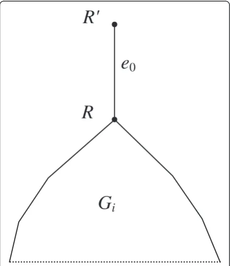
wherev'is the parent vertex ofv. The root of the tree is considered good if the first condition in (4) is true. Now letGjbe polytomous. We assume thatGjcontains an additional edgee0located upwards from the root as shown in Figure2. Given a setV∈P, a vertexvof treeGjis called
good(with respect toV) if at least one of its children obeys condition (4) or the first condition in (4) if vis the super-root. For each setV∈P, theset R(V) of good vertices in all source gene treesGjis composed. If a binary treeGjis also considered polytomous, these two definitions give, generally
defining, different sets of good vertices but of equal cardinality. It is enough, as only the cardinality of the setR(V) is considered further.
I.4)Finding basic sets and their partitions in the set P.
For each fixed non-singleton basic setV(inP), all partitioning variants are considered, i.e., all variants defined by the equalityV = V1+V2, where non-empty disjoint setsV1,V2are themselves basic.
I.5)Building basic trees S(V)and computing their costs.
For each basic setV, the basic treeS(V) along with its costc(V) is defined and computed by induction. The treeS(V) for a singleton setVconsists of one root-leaf vertex assigned a species fromV; the cost
c(V) of thisS(V) is zero. The induction step for a fixedV: for each partition variantV = V1+V2the valuec(V1,V2) =c(V1) +c(V2) +Cd+Clis Table 1 Types of evolutionary events and their costs(Continued)
24 same as #23 tr_rl geneetransfers without retention tod' ~ d, d'≠d*, that bifurcates intod'1andd'2, thene1 transfers tod'2, ande2–tod'1
с=c(e1,d'2)+c(e2,d'1)+c(tr_without)
(minimization overd', if uncertainty select one closest tod)
25 e≠e0, edgeebifurcates intoe1 ande2,d≠d*
ga_lr geneeemerges in speciesd' ~ dthat bifurcates intod'1andd'2, thene1transfers tod'1, and
e2–tod'2
с=c(e1,d'1)+c(e2,d'2)+c(gain) (minimization overd')
26 same as #25 ga_rl geneeemerges in speciesd' ~ dthat bifurcates intod'1andd'2, thene1transfers tod'2, and
e2–tod'1
с=c(e1,d'2)+c(e2,d'1)+c(gain) (minimization overd')
27 d≠d*,d≠d0 tr_l geneetransfers without retention to species
d' ~ d, d'≠d* that bifurcates intod'1andd'2, and then transfers tod'1and is lost ind'2
с=c(e,d'1)+c(tr_without)+c(loss) (minimization overd', if uncertainty select one closest tod)
28 same as #27 tr_r geneetransfers without retention to species
d' ~ d, d'≠d* that bifurcates intod'1andd'2, and then transfers tod'2and is lost ind'1
с=c(e,d'2)+c(tr_without)+c(loss) (minimization overd', if uncertainty select one closest tod)
29 e≠e0, d=d* ga_l geneeemerges in speciesd' ~ dthat bifurcates intod'1andd'2, and then transfers tod'1and is lost ind'2
с=c(e,d'1)+c(gain)+c(loss) (minimization overd')
30 same as #29 ga_r geneeemerges in speciesd' ~ dthat bifurcates intod'1andd'2, and then transfers tod'2and is lost ind'1
с=c(e,d'2)+c(gain)+c(loss) (minimization overd')
31 edgeebifurcates intoe1ande2,
d≠d*,d≠d0
tr_dupl geneetransfers without retention to species
d' ~ d, d'≠d*, and then duplicates
c=c(e1,d')+c(e2,d')+c(tr_without)+c(dupl) (minimization overd', if uncertainty select one closest tod)
32 edgeebifurcates intoe1ande2,
e≠e0, d=d*
ga_dupl geneeemerges in speciesd' ~ d,and then duplicates
c=c(e1,d')+c(e2,d')+c(gain)+c(dupl) (minimization overd')
33 edgeebifurcates intoe1ande2,
d≠d*,d≠d0
tr_double geneetransfers without retention to species
d' ~ d, d'≠d*, then its copye2transfers tod”~ d,
d”≠d”,d”≠d*, and copye1–tod'; or vice versa replacingd'withd"ande1withe2
c=c(e1,d')+c(e2,d")+c(tr_without)+c(tr_with) (minimization over pair <d', d">, if uncertainty select a pair closest todas per the sum of distances)
34 e≠e0, edgeebifurcates intoe1 ande2,d=d*
ga_double geneeemerges in speciesd' ~ d,then its copy
e2transfers tod" ~ d, d"≠d', and copye1retains ind'; or vice versa replacingd'withd"ande1 withe2
c=c(e1,d')+c(e2,d")+c(gain)+c(tr_with) (minimization over pair <d’, d">)
Considerias the number of the event (and the row number) in a fixed enumeration pattern;“Condition”defines the applicability of the event to current pair <e,d>;“Name”is the event type;“Description”is the event synopsis;“Cost”contains formulas to compute the costs of scenarios initiated from an event in a current row. A notationd~d'designates that“tubesdandd'differ and belong to the same time slice”. The constantsc(dupl),c(loss),c(gain),c(gain_big),
computed, and the minimum (over all partitions ofV).
c Vð Þ ¼ minfc Vð 1;V2ÞjV ¼V1þV2g
is found, where Cd is the total cost of duplications on
edge V (we equally denote by V the set of leaf species, the root edge and the root vertex of the corresponding subtree), and Cl is the total cost of losses on edges V1
andV2, see Figure3. BothCdandClare defined below.
A partition <V1,V2> that minimizes the functionalc(V)
over all partitions of V is called the minimal partition
(of V). Once the minimal partition is found, the tree S
(V) is obtained by joining treesS(V1) andS(V2) and
root-ing them at the joint vertex and edge, as shown in Figure 3.
Thus, to calculate the total costsCdandCl, aset r(V1, V2) of vertices v in all Gj is constructed such that one
child vertex of vbelongs to R(V1), and the other –to R
(V2) (ifvis binary). A polytomous vertexvis included in r(V1,V2) ifvpossesses at least one child satisfying (4) for V1and one satisfying (4) for V2. The total cost of
dupli-cations on edge Vis calculated as Cd=cd · (|R(V1)|+|R
(V2)|–|R(V)|–|r(V1,V2)|), where | | denotes the
cardinal-ity of a set, andcdis the cost of one duplication (the
al-gorithm parameter). The total cost of losses in edgesV1
and V2is calculated as Cl =cl · (|R(V1)|+|R(V2)|–2|r(V1, V2)|), where cl is the cost of one loss (the algorithm
parameter).
Additionally, the weight of the tree S(V) is calculated with the formula
w Vð Þ ¼ 1þca
m
c V0
c Vð Þ
c Vð Þ0
where a is the number of leaves in S(V), m is the total
number of species, andcis the algorithm parameter
(de-fault isc=10). Here the partitionV'is closest to the min-imal partition in terms of the cost; if no other partition exists, it is assumed thatw(V) = 1. The weights are used at Phase II of the algorithm.
Phase I (steps I.1-I.5) ends with removing all basic trees containing less than 3 leaves. The obtained set of weighted basic trees is the outcome of Phase I of the first algorithm.
Operating time of Phase I for the standard P has the
order ofO((n·m)3), and for anyP–the order isO(|P|3+ |P|2nm). A rigorous cubic complexity and mathematical proof (in the special common case) are the advantages of the Phase I algorithm comparing to known heuristic methods.
II) The second phase of the first algorithm (Phase II).
This phase is heuristic. For any species tree S with the
leaves-species set W and the basic tree S(V), define the
cost c(S(V),S) as the cost of mapping α or β of the tree
S'(V) intoS(the cost ofβis defined in see Computing the total cost of binary gene trees against the species tree below). Here, S'(V) is obtained from S(V) by pruning all
R'
R
G
i
e
0
Figure 2An additional“root”edge between the“super-root”R' and the initial rootRin treeGj.This root is used to define the set
R(V), since the vertexR'can be good. The root edgee0is analogous to the root tubed0in Figure 1.
S
(
V
)
S
(
V
1)
S
(
V
2)
V
1V
2V
Figure 3TreeS(V) for a fixed partitionV=V1+V2.HereV,V1,V2 designates both the corresponding vertex and the edge upwards from this vertex. TreesS(V1) andS(V2), as well as their costsc(V1) and
c(V2), are already known from induction, andCd+Clcorresponds to
leaves containing species outside W together with their edges.
The cost c(S) of any species tree S is defined as the sum of costs c(S(V),S) over all basic trees S(V), or, op-tionally, each cost is multiplied byw(V). Thus,
c Sð Þ ¼X S Vð Þ
w Vð Þ:c S Vð ð Þ;SÞ
where summation is done over all basic trees S(V) or,
equally, over all basic setsVwith cardinality higher than or equal to 3. As above, let V0be the set of all species
contained in leaves of allGj.
The initial step of Phase II.The algorithm enumerates all triplet-leaved trees S with three leaves-species from
V0 and selects one with the minimal cost c(S). This S
constitutes the seed partial supertree in the below procedure.
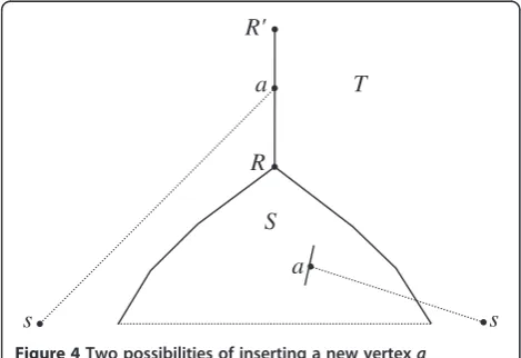
The inductive step of Phase II. In the current partial supertreeS with the setWof leaves-species (a subset of
V0), each edge is attempted for insertion of a new vertex
a connected to a species s from V0, and for placing a
new root a above the current root, Figure 4. Among
such possible extensions T of S, we choose the tree T
with the minimal cost с(T); it supersedes the current
partial supertree S. Extensions are attempted until all
species fromV0are added to the current treeS, and the
algorithm halts. The eventual S is the sought-for
super-treeS*. The end of Phase II.
Additional file 1 contains a more detailed description of Phase II, including the assessment of vertex reliability
in the final supertree and overall supertree reliability. It also presents a simplified version of Phase II.
The second algorithm: reconciliation of gene and species trees and building evolutionary scenarios
Given are a set {Gj} of rooted polytomous gene trees
(paralogs are allowed), a rooted binary species treeSand
a treeS0obtained fromSby inserting one or several
ver-tices into tubes to delimit time slices, Figure 1. EachGj
and the tree S0 are attributed the root edge e0 and the
root tubed0as depicted in Figure 2. If the indexj is
ir-relevant,Gjis equivalent toG.
The set of species is fixed, with one “accessory” out-group leafd* added to the tree root. For the species tree, the notations of terminal tubes, leaves and speciesx (in-cluding the outgroup) are unified to define identical objects. For gene trees, the identical objects are terminal edges, leaves and leaf notationsx-y. The correspondence between leaf notationsx-yinGandxinSandS0is fixed
as the gene-species correspondence (gene “y” exists in
species“x”).
The second algorithm refers to a complex of algo-rithms to solve four separate problems as described below in Computing the total cost of binary gene trees against the species tree - Stochastic characteristics of the second scenario design.
Ordering used in the algorithm
All gene trees Gj are enumerated (indexj can be
omit-ted). Under a fixedj, triplets <e,d,i> are enumerated as follows. EdgeseinGare visited in the order of descend-ing distance from the root (from deeper to shallower levels), and from left to right within the same level. Tubesdin S0are visited in the order of descending the
level of the time slice (upwards to the root). Within a slice, for each e ≠e0tubes are visited from left to right
starting from the outgroup d*, and for the root edge e0
the left-to-right visiting ends with the outgroupd*. Here
d* is a segment of the outgroup tube in tree Sthat falls within the current time slice. Next, the 35 types of gene
evolution events i are visited in the order specified in
Table 1, withirunning from 0 to 34.
All trees G considered (see Conclusion) are binary.
Encountered polytomous trees are binarized. The binari-zation procedure is described in Additional file 2.
Computing the total cost of binary gene trees against the species tree
In Table 1, each row provides the event name and de-scription (third and fourth columns, respectively), and the last column defines the cost of <e,d,i>.
Letjspecify the treeG,erun over its edges, anddrun over tubes inS0. Define
cminðe;d;jÞ ¼cminðe;dÞ ¼minic eð ;d;iÞ ð5Þ
where с(e,d,i) is the cost specified in the last column of Table 1 if the current pair <e,d>satisfies the condition de-fining the particular event type. In computingсmin(e,d) the
arguments <e,d>are enumerated according to the order-ing specified in The second algorithm: reconciliation of
S
a
a
s
s
T
R'
R
gene and species trees and building evolutionary scenar-ios. Figure 5 exemplifies an induction step.
The minimum of (5) is attained at the“minimal”event (the “minimal” row in Table 1) i. Certain events imply the minimization over the variable tubed'or the pair of tubes <d',d">; the minimal value of the variable is re-ferred to as the“minimal parameter”.
The value сmin(e0,d0) is denoted as c(G,S), recall that G=Gj. The value
X
j
cminðe0;d0;jÞ is denoted asc({Gj}, S) and referred to as the total cost of the input set {Gj}
of binary gene trees against the treeS. Thetotal costof the supertreeS*is denoted asc({Gj},S*).
The value сmin(e, d) can be interpreted as a “
condi-tional cost”, i.e. the cost of an optimal evolutionary
sce-nario if it initiates from edge e in tube d and evolves
into terminal leaves with cohered pairs of genes-species.
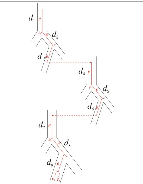
First scenario design: the event tree
Each treeG(or its binarizationG') is associated with the
first scenario(the event tree) Tof the evolution of gene
Galong the species treeS0. The tree vertices correspond
to certain pairs <e,d>, the root–to the pair <e0,d0>, the
leaves–to pairs formed with a terminal edge and a
ter-minal tube obeying the “species-gene”relation. The tree edges can be unary (ordinary) or binary, i.e., pairs of unary edges originated from a single vertex. The algo-rithm of constructingToverGis similar to the binariza-tion procedure detailed in Addibinariza-tional file 2.
During the forward run (described in Computing the total cost of binary gene trees against the species tree) each pair <e,d> is assigned the minimal eventiaccording to (5)
and its minimal parameters. The backward run starts from the pair <e0,d0>. At each step either a binary edge is
pro-jected from vertex <e,d> into vertices denoted as <е1,d'1>
and <е2,d'2> (case 1), or a unary edge is projected into
ver-tex <e,d'> (case 2), whered'1,d'2,d'are the minimal
para-meters. The edge is tagged with the event namei. Case 1 implies a bifurcation resulted from the minimal event.
By definition, the cost of the first scenarioTis the cost of the input treeGagainstS0, i.e.c(T) =c(G, S0). It can
be detailed with the amounts of different event types in-ferred in tubes of the species tree, the total amount of events, the individual event costs, etc.
Themappingβis equivalent toT, and the cost ofβis equal to the cost of Tas substantiated below. It is easy
to show that for each е in G there are vertices inT of
the form <e,d> with different tubesd. Each such tube
d1,. . .,dl is associated inTwith the unique
correspond-ing eventitthat occurred on edgeeinside tubedt(such it tags the unique edge originated from vertex <e, dt>
inT). By definition,β(e)={d1,. . .,dt,. . ., dl}. The setβ(e)
can be interpreted as a path. Consider first d1 that is
closest to the root inS0. If tubesdtanddt+1are
compar-able then dtis closer to the root, otherwisedt+1accepts
a transfer from dt (Figure 6) or dt+1 is a child of the
accepting tube. The set β(e) forms in S0 a connected
path defined by the scenarioTand consisting of
repeti-tions of edgeeand transfers without retention. This def-inition of β(e) requires a clarification: events it are
determined by β(e) and S0, except for the last event il.
Therefore, β(e) can be expressed as β(e)={d1, . . ., dl; il}.
For mappingβlet us definec(β) =c(T).
The event treeTcan be easily recovered with a known
β, which is however not of interest becauseTis used as
G
G
1G
2e
1e
2e
G
1G
2e
1e
2e
e
c
(
G
1,
S
)
c
(
G
2,
S
)
d
d'
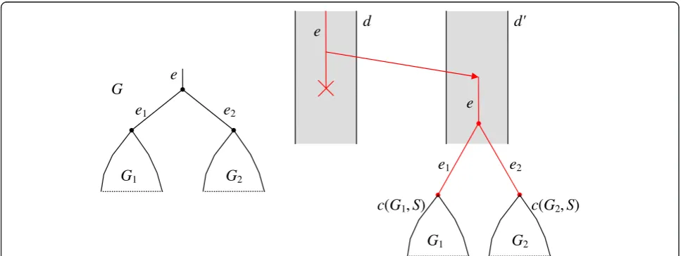
Figure 5The inductive step in computing the costc(G,S).On the left is an illustration of assembling the treeGfrom subtreesG1andG2. Here
e
1 2
d
1
d
2
d
3
d
4
d
5
d
6
d
7
d
8
d
9
e
e
e
e
e
e
e
e
e e
the first scenario. Note thatβis the global minimum of the cost functionalc(f), where fis any admissible
distri-bution of edges in G along tubes in S0; we omit exact
definitions here.
Second scenario design: a random process on the graph
In First scenario design: the event tree, the scenario Tis constructed during consecutive selection of minimal events in the tubes. However, the discarded alternatives may represent events with just slightly higher costs. As true event costs are unknown, it becomes an important consideration. We describe a novel approach to construct the scenario as a random process on the graph, which allows us to take suboptimal scenarios into account.
Fix a natural number k (the “degree of ramification”, the algorithm parameter).
For each G, construct a directed acyclic graph(DAG)
Rwith unary and binary edges, vertices corresponding to
pairs < e, d >, and the root < e0, d0 >. The edges are
tagged with event names i1, . . ., il (where l ≤ k) from
Table 1. During the forward run of the algorithm, unlike with the first scenario (event tree)T, not one butk“best” (in terms of the cost) unary or binary edges are pro-jected from each vertex < e, d > and tagged with the event i, i.e. i takes kor less values at each vertex. Each edge is assigned conditional probability piand
uncondi-tional probability p(e, d, i) of undergoing evolutionary
events i. Under k = 1 the evolution is deterministic,
i.e., the probabilities are either 0 or 1, and edges receiv-ing the probability of 1 constitute the first scenarioT.
Leaf pairs < e, d> cohered by the “species-gene” cor-respondence constitute the leaves in DAG, with no out-going edges. A non-cohered pair < e, d > projects an edge into the cohered pair <e, х>, where xis the tube that terminates with the species assigned to the leaf e.
This edge is tagged with the probability pi=1 and the
row number 1 (Table 1). A pair <e,d*> also projects an edge into a cohered pair <e,х>; the edge is tagged with
pi=1 and the row number 2 (Table 1).
The above paragraph describes the start of induction in the construction of DAG. The induction step is more sophisticated and is described in Additional file 2.
Intuitively, DAG describes the evolutionary branching of a gene described by the treeGalong a species described by the treeS. For eachG, the value p(e,d, i) assigned to the DAG edge <e,d,i> is a probability of inclusion of the edge into the event tree. Starting from vertex < e0, d0>
and arriving into < e, d >, choose its i-th outgoing edge with the probabilitypi. If a unary edge is chosen, proceed
to its terminus; if a binary edge is chosen, the process bifurcates into the termini of the edge.
Note that the lower the cost c(e, d, i), the higher the
probability pi. For the second scenario, the algorithm
computes not the cost but the expectation of the
number and total cost of various event types. The
expec-tations depend on parameter k, which default value is
10. Computer simulations show that higher k produce
similar expectations.
The first scenario is the best in terms of the cost, the second scenario incorporates a number of good solu-tions (the threshold set indirectly byk). Underk= 1 the scenarios coincide, and cost expectations coincide with the costs. Under k> 1 the second scenario is a refine-ment of the first scenario. E.g., if duplications in the root tube are absent in the best scenario but present in sub-optimal solutions, the second scenario will show their expectation already atk= 10.
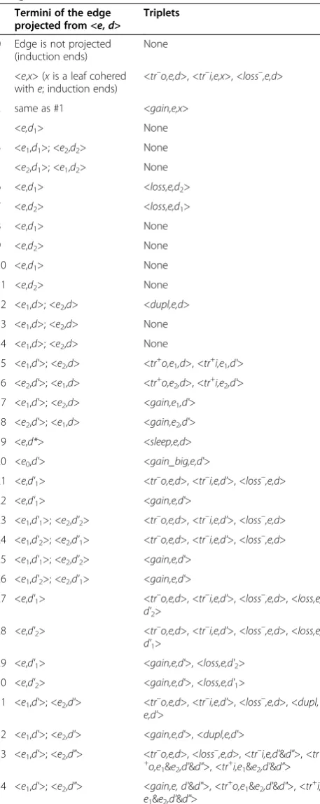
Stochastic characteristics of the second scenario design
Denote anI-typea fixed setIof tags selected by the user. The third column of Table 2 contains the following tags:
gene gain (gain), origin of the common ancestor of all
genes (gain_big), gene duplication (dupl), gene loss
(loss), gene transfer from a tube with retention (tr+o), gene transfer from a tube without retention (tr–o), gene transfer into a tube with retention (tr+i), gene transfer into a tube without retention (tr–i), loss of the trans-ferred copy in the donor (loss–). Other tags can be added to define event types in terms of DAG.
Denote aT-type a set T of edges with all descendant
leaves marked with * in one or several trees Gj (a
dis-junctive union over j). An example is a set of ancestral ribosomal or mitochondrial genes.
Letube a fixed tube. The given setIand tubeudefine the set X of edges inRj: edge iin DAG is included inX
if one of the triplets at the intersection of the third
col-umn and thei-th row in Table 2 contains the first
mem-ber belonging to Iand the third member being the tube
u. Denote this condition i ∈ I,u. Note that the second
and third members of any triplet are uniquely deter-mined by the terminus/termini of edgei, ref. to Table 2.
Analogously, given sets I and T define the set X of
edges inRj: edgeiin DAG is included inXif one of the
triplets at the intersection of the third column and the
i-th row in Table 2 contains the first member belonging
to I and the second member being an edge from T.
Denote this conditioni∈I, T.
Compute expectations of the parameters of the sto-chastic process described in Second scenario design: a
random process on the graph, the “amount of events
fromIin tubeu” f(I,u) and the “amount of events from
Ion edges fromТ”g(I,Т):
f Ið ;uÞ ¼X j
X
e;d
X
<e;d>→i; i∈I;u
p eð ;d;j;iÞ
in the notationd'&d" the summands foru = d'oru = d"
are halved.
For the givenIandТthe value ofg(I,Т) is
g Ið;TÞ ¼X j
X
e;d
X
<e;d>→i; i∈I;T
p eð ;d;j;iÞ
Ifiis one of the last two rows in Table 2, then in the no-tationе1&е2the summands fore1∈Tore2∈Tare halved.
In some cases, one may be interested to know the mathematical expectation of the total cost of events rather than their amount. The expectations are obtained using the formulas:
cf Ið ;uÞ ¼X j
X
e;d
X
<e;d>→i; i∈I;u
ci:p eð;d;j;iÞ
cg Ið ;TÞ ¼X j
X
e;d
X
<e;d>→i; i∈I;T
ci:p eð ;d;j;iÞ
Under k =1 all expectations equal the number of
events or the cost values.
More general characteristics can also be estimated, such as the sum
X
u;i∈I
cf Ið;uÞ ð6Þ
of expectations of the event costs over all tubesuand all events i from I, where I includes the gene gain (gain),
origin of the common ancestor of all genes (gain_big),
gene duplication (dupl), loss (loss), transfer from a tube (tr–oилиtr+o), loss of the transferred copy in the donor (loss–). Other setsIcan be used in (6).
Denote the sum (6) as the cost of the second scenario.
Results and discussion
The models and algorithms described in the Methods are original developments of the authors and largely comprise the results of the study. This section details their implementation, testing on various data, and other relevant results.
Implementation of the first algorithm
The Super3GL program accepts a set of rooted gene treesGj, which are allowed to contain polytomous
verti-ces (ref. also to Additional file 1).
The program produces a supertree that amalgamates the set of input trees, allowing for duplications, gains, losses and horizontal transfers as evolutionary events, and imposes no condition onP(e.g. condition (*)); thus, the program realizes the heuristic algorithm described in Description of the first algorithm.
The input and resulting trees are in the Newick paren-thesis format. If requested, the reliability of each super-tree vertex is included in the super-tree notation as a length of
Table 2 Definitions of events in the second scenario design (in the DAG)
i Termini of the edge projected from <e,d>
Triplets
0 Edge is not projected (induction ends)
None
1 <e,х> (хis a leaf cohered withe; induction ends)
<tr–o,e,d>, <tr–i,e,х>, <loss–,e,d>
2 same as #1 <gain,e,х>
3 <e,d1> None
4 <e1,d1>; <e2,d2> None
5 <e2,d1>; <e1,d2> None
6 <e,d1> <loss,e,d2>
7 <e,d2> <loss,e,d1>
8 <e,d1> None
9 <e,d2> None
10 <e,d1> None
11 <e,d2> None
12 <e1,d>; <e2,d> <dupl,e,d>
13 <e1,d>; <e2,d> None
14 <e1,d>; <e2,d> None
15 <e1,d'>; <e2,d> <tr+o,e1,d>, <tr
+
i,e1,d'>
16 <e2,d'>; <e1,d> <tr+o,e2,d>, <tr
+
i,e2,d'>
17 <e1,d'>; <e2,d> <gain,e1,d'>
18 <e2,d'>; <e1,d> <gain,e2,d'>
19 <e,d*> <sleep,e,d>
20 <e0,d'> <gain_big,e,d'>
21 <e,d'1> <tr–o,e,d>, <tr–i,e,d'>, <loss–,e,d>
22 <e,d'1> <gain,e,d'>
23 <e1,d'1>; <e2,d'2> <tr–o,e,d>, <tr–i,e,d'>, <loss–,e,d>
24 <e1,d'2>; <e2,d'1> <tr–o,e,d>, <tr–i,e,d'>, <loss–,e,d>
25 <e1,d'1>; <e2,d'2> <gain,e,d'>
26 <e1,d'2>; <e2,d'1> <gain,e,d'>
27 <e,d'1> <tr–o,e,d>, <tr–i,e,d'>, <loss–,e,d>, <loss,e, d'2>
28 <e,d'2> <tr–o,e,d>, <tr–i,e,d'>, <loss–,e,d>, <loss,e, d'1>
29 <e,d'1> <gain,e,d'>, <loss,e,d'2>
30 <e,d'2> <gain,e,d'>, <loss,e,d'1>
31 <e1,d'>; <e2,d'> <tr–o,e,d>, <tr–i,e,d'>, <loss–,e,d>, <dupl, e,d'>
32 <e1,d'>; <e2,d'> <gain,e,d'>, <dupl,e,d'>
33 <e1,d'>; <e2,d"> <tr–o,e,d>, <loss–,e,d>, <tr–i,e,d'&d">, <tr
+
o,e1&e2,d'&d">, <tr
+
i,e1&e2,d'&d">
34 <e1,d'>; <e2,d"> <gain,e, d'&d">, <tr+o,e1&e2,d'&d">, <tr
+
i, e1&e2,d'&d">
the incoming edge; the general reliability of the super-tree can also be computed.
Super3GL is written in C++ as a command-line utility and optionally accepts a configuration file to avoid re-typing non-default arguments. As mentioned above, the
algorithm consists of two phases. Phase I, which builds
a set of basic trees, cannot be interrupted. Phase II,
which builds the final supertree from the set of basic
trees incrementally by induction, is independent from the first phase and can be interrupted and resumed at any time.
The program automatically detects the MPI environ-ment of version 1.2 or above; in which case it runs the parallel version of the algorithm. Detailed information about the program performance and scalability is given in the user’s manual.
Both 32-bit and 64-bit versions of Super3GL were tested on MS Windows and Linux on a stand-alone
computer with 1–4 CPUs, as well as on the MVS-100K
cluster of the Joint Supercomputer Center of the Russian Academy of Sciences [21] using up to 2048 CPUs.
The source code of Super3GL for Linux can be obtained free of charge from the Web page [19] under the GNU General Public License version 3.
Implementation of the second algorithm
Embed3GL implements all operations discussed in The second algorithm: reconciliation of gene and species trees and building evolutionary scenarios. The program inputs a set of gene treesGjthat are allowed to contain
polytomous vertices and paralogs. All trees are rooted, otherwise the algorithm from Additional file 1 is pre-applied.
The original species treeSand its modified versionS0
are provided as one tree: the name of each vertex in the
parenthesis notation ofS is followed by an integer
num-ber, the “length” of the incoming tube. This value indi-cates the number of “new” tubes in S0 that form in the
place of the“old”tube inSby inserting additional verti-ces. The default length of 1 means that no new vertex is inserted. A separate program, also available at the Web page [20], can be applied for time-slicing of a given spe-cies tree, which will be converted into the required tree format.
Each new tube d is attributed to a certain old tube,
d¼d dð Þ. It allows to compute characteristics of the old tube based on those of new tubes, which is frequently of
interest. For instance, one may need X
d∈d
f dð Þ, where
d∈d means that the new tube dis a part of the old tube
d¼d dð Þ, andfis the desired characteristic.
The Embed3GL program is written in C/C++ as a command-line utility and optionally accepts a
configu-ration file to avoid re-typing of non-default arguments. The program automatically detects the MPI environ-ment (version 1.2 or above), in which case it impleenviron-ments an effectively parallelized version of the algorithm.
The input gene trees are provided in the Newick par-enthesis format as one or several files; the species tree is provided in the same notation in a separate file. All operations mentioned in The second algorithm: recon-ciliation of gene and species trees and building evolu-tionary scenarios can be performed serially or in any desired combination.
The Embed3GL program executables for 32/64-bit
Windows along with the user’s manual and usage
exam-ples are freely available at the Web page [20]. The source code for Linux can be obtained free of charge from the same page under the GNU General Public License ver-sion 3.
Testing of the algorithms
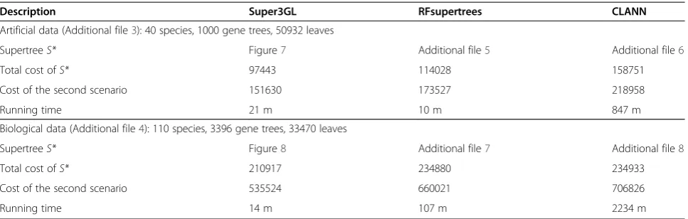
The Super3GL performance and results were compared against recognized supertree building programs on artifi-cial and biological data. All comparisons were done in the uniprocessing mode on an Intel Xeon 2.0 GHz plat-form. Stochastic programs were run several times and the best result of the series was used for comparison. Super3GL was run once because its algorithm is deter-ministic. Selected comparisons with RFsupertrees [5] and Clann version 3.0.2 [22] are presented in Table 3. All programs were run with default parameter settings.
The three programsused the same input filesprovided
in Additional file 3 (artificial data) and Additional file 4 (biological data).
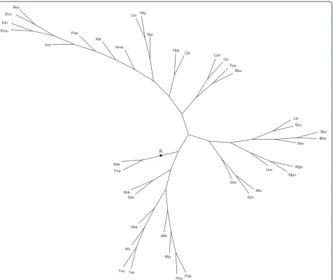
Algorithms comparison with artificial data
Artificial trees were randomly generated from a known species tree S*. An exampleS* with 40 leaves is given in
Figure 7. An example set {Gj} of 1000 generated gene
trees is given in Additional file 3. Trees contain 50,932 leaves in total. The method used to generate gene trees on a given species tree is described in [8], p. 166. As mentioned below, the procedure of trees simulation along a topology needs further study and justification.
Super3GL reconstructed the known species tree in
95% cases, S = S*. The two other programs used the
same set of input trees but often constructed supertrees essentially different fromS*; ref. e.g. to Additional files 5 and 6. The total costs of mapping of {Gj} into S are as
well presented in Table 3.
On the Robinson-Foulds distance
study) in terms of minimizing this functional. In essence, this functional is a measure of distance between the given set {Gj} and the supertreeS.
Different approaches to measure this distance are known.
Thus, theRF-functional RF Gj ;S
¼X
j
RF Gj;S
is a
sum of Robinson-Foulds distances [5,23] betweenGjandS
over allGj. A rigorous comparison between the functionals RF({Gj},S) over allGj. A rigorous comparison between the
functionals RF({Gj}, S) and c Gj ;S
¼X
j
c Gj;S
requires a separate systematic study. Below are some pre-liminary considerations.
Assume that tree S contains the set of leaves V0, and
consider only species notations in leaves ofGj. Typically,
each Gj contains less species than S, and computing a
RF-distance requires pruning of certain amount of
spe-cies from S for each current Gj. Properties of the RF
-functional need to be studied.
Under the absence of paralogs, the minimization of theRF-functional is equivalent to maximization of clades
matching between the topologies of Gj and S. In terms
of mappingα, it is the maximization of cases when only
one edge of the gene tree enters a tube of the species tree (i.e. the edge origin is mapped into the tube origin
or earlier, and the edge terminus – into the tube or
later). In biological terms, this speciation event is not associated with acquisition of paralogs. The authors are
unaware of any research that interprets the RF-measure
in terms of gene evolution events.
As with the mapping cost, the problem of minimizing the RF-functional is NP-hard, unless the tree Scontains
only clades belonging to a pre-defined setP. When this
non-standard statement is assumed, the problem is solved with our algorithm exactly as described in this study for the cost functional. The proposed algorithm is universally applicable to any functional defined in terms
of mapping edges. A natural example in case of paralogs is the minimization of the total amount of edges that enter tubes of the species tree. The described cost
func-tional performs better than RF-functional even in the
special case, where only gene duplications and losses are considered.
Algorithms comparison with biological data
Biological datais a set of unrooted gene trees provided by the courtesy of Prof. James McInerney (National Uni-versity of Ireland, Maynooth). The trees were rooted using the procedure described in Additional file 1 to ob-tain the set of 3396 gene trees for 110 prokaryotic spe-cies. The trees contain 33,470 leaves in total. The set is provided in Additional file 4.
The supertree built by Super3GL is shown in Figure 8. It coincides mainly with the species tree from [24], with the same differences as between the tree of [24] and a later genomic tree of [25], which suggests support for our supertree building method. Supertrees built by the two other programs (ref. to Additional files 7 and 8) es-sentially differ from the mentioned trees [24,25].
Trees presented in Figure 8 and Additional files 7, 8 were not manually edited.
A comparative biological interpretation of our
obtained supertree and the topology of other two trees also favors the Super3GL result. Consider four widely accepted phylogenetic patterns:
1) Archaebacteria and Eubacteria form two separate basal domains;
2) Spirochaetes are monophyletic within Eubacteria; 3) Bacilli, Clostridia, Lactobacilli,Mycoplasmaand
other Mollicutes constitute a separate monophyletic lineage within Eubacteria;
4) Proteobacteria are monophyletic within Eubacteria and contain the monophyletic subclade ofα-Proteobacteria.
Table 3 Comparison of Super3GL with RFsupertrees and CLANN version 3.0.2
Description Super3GL RFsupertrees CLANN
Artificial data (Additional file3): 40 species, 1000 gene trees, 50932 leaves
SupertreeS* Figure7 Additional file5 Additional file6
Total cost ofS* 97443 114028 158751
Cost of the second scenario 151630 173527 218958
Running time 21 m 10 m 847 m
Biological data (Additional file4): 110 species, 3396 gene trees, 33470 leaves
SupertreeS* Figure8 Additional file7 Additional file8
Total cost ofS* 210917 234880 234933
Cost of the second scenario 535524 660021 706826
Running time 14 m 107 m 2234 m
The tree in Figure 8 represents all four patterns. The tree in Additional files 7 contains only pattern 4, but splits Archaebacteria into a paraphyletic grade, separates spiro-chaetes (Borrelia, Leptospira, Treponema) among three distant lineages, places Clostridia+Mollicutes and Bacilli +Lactobacilli into different clades, the latter also contain-ing a spirochaeteTreponema. The tree in Additional file 8 does not show any of the four patterns: Archaebacteria are not basal, Spirochaetes largely intermix with other
bacteria, Phytoplasma and Clostridia enter the Archaebac-teria clade, Bacilli and Lactobacilli are mixed with
Bacter-oidetes,Mycoplasma–with selected Chlamydiae, mostα
-Proteobacteria are scattered between early diverging lineages,RickettsiaandEhrlichiaare placed in two differ-ent distant clades. All trees, however, show minor devia-tions from the biologically expected topology at a more shallow level. Thus, Leifsonia is always placed closer to
Bifidobacterium than to other actinomycetes; in Figure 8
R
Figure 7The artificial species treeS* used to simulate sets {Gj} of gene trees (40 species).The tree root is denoted byR. One of the simulated sets {Gj} is presented in Additional file 3. The Super3GL program applied to {Gj} reconstructed the known supertreeS* in 95% cases. The
total mapping cost equals 97443. Leaf notations: Archaea:Archaeoglobus fulgidus(Afu),Halobacterium sp. NRC-1(Hbs),Methanococcus jannaschii
(Mja),Methanobacterium thermoautotrophicum(Mth),Thermoplasma acidophilum(Tac),Thermoplasma volcanium(Tvo),Pyrococcus horikoshii(Pho),
Pyrococcus abyssi(Pab),Aeropyrum pernix(Ape),Sulfolobus solfataricus(Sso); Gram-positive bacteria:Streptococcus pyogenes(Spy),Bacillus subtilis
(Bsu),Bacillus halodurans(Bha),Lactococcus lastis(Lla),Staphylococcus aureus(Sau),Ureaplasma urealyticum(Uur),Mycoplasma pneumoniae(Mpn),
Mycoplasma genitalium(Mge);α-Proteobacteria:Mesorhizobium loti(Mlo),Caulobacter crescentus(Ccr),Rickettsia prowazekii(Rpr);β-Proteobacteria:
Neisseria meningitidis MC58 (Nme);γ-Proteobacteria:Escherichia coli K12(Eco),Buchnera sp. APS(Buc),Pseudomonas aeruginosa(Pae),Vibrio cholerae
Pasteurellaceae enter Enterobacteriaceae. Such artifacts might indicate sampling errors of the data in Additional file 4.
Compare the evolutionary scenario designs defined in Methods. The two designs are compared in Table 4 on the basis of the same set of input gene trees.
Table 3 (the“cost of second scenario” row) details the comparison of the three programs. Note that comparing programs against the first and second scenarios pro-duces the same result. Example expectations of the total
(over all tubes) event costs for the two scenarios are given in Table 4.
Analyses used the NCBI taxonomy [26]. Trees were visualized with TreeView [27] and Dendroscope [28].
The rooting algorithm for unrooted trees is trivial and explained in Additional file 1.
Conclusions
The problem of optimal amalgamation of a set of trees has a long history. This problem can be generalized into
Ρ
1
2
3
4
α
searching for an“average”graph of a given set of graphs. In the phylogenetic context, that will describe the desired supertree. Such graph will globally minimize the total sum of differences between each reconciled tree and the supertree. Pioneer studies (ref. to [2] and further references provided therein) defined the difference be-tween the trees Gand Sin terms of the cost с(G, S) of
mappingαof one tree into another. Under this concept,
searching for a supertree was naturally viewed as
search-ing for the global minimum of the functional
X jc Gj;S
referred to as thecostof the amalgamation
of treesGj.
The set of admissible trees Swas not always explicitly specified for this functional. Its minimum was implied to
be found among all species trees that contain species
present in all amalgamated input trees. Under this state-ment, the problem cannot be rigorously solved in poly-nomial time.
We suggest a reformulation to search for the supertree among species trees that contain clades present in the set of input trees or, more generally, belonging to a
pre-defined set Р. We developed a deterministic algorithm
that finds the supertree for any givenPin the time cubic
of |P|. Moreover, for a special common case the
algo-rithm was mathematically proved to find exactly the glo-bal minimum of the total amalgamation cost.
The software implementation of the developed algo-rithm performs faster and more accurately comparing to known tools of inferring supertrees. Empirical testing was done with artificial and biological data. However, for its rigorous statistical verification a sound comparative framework to cross-test supertree building algorithms is still to be developed.
Of basic importance to approach the tree amalgam-ation problem is to define evolutionary events that can biologically explain a correct amalgamation. The authors developed a detailed list of such events, which is far
more extensive than found in current literature. The ul-timate definition of an evolutionary scenario will require further research. We suggest two approaches to build scenarios. Their corresponding algorithms are mathem-atically proved and possess a cubic complexity to the in-put data size.
Additional files
Additional file 1:Rooting algorithm for unrooted trees. Computational complexity of the first algorithm and reliability of the supertree. Alternative design of Phase II.
Additional file 2:Transition from a polytomous to binary tree. Inductive step of constructing a directed acyclic graph.
Additional file 3:Input gene trees (artificial data).(viewable by e.g. TreeViewX).
Additional file 4:Input gene trees (biological data).(viewable by e.g. TreeViewX).
Additional file 5:Supertree built by RFsupertrees for artificial data from Additional file3.In the unrooted topology, the two outlined subtrees swapped with respect to the correct tree in Figure 7. The total mapping cost is 114028.
Additional file 6:Supertree built by CLANN version 3.0.2 for artificial data from Additional file3.In the unrooted topology, the two set-off edges are misplaced with respect to the correct tree in Figure 7. The total mapping cost is 158751.
Additional file 7:Supertree built by RFsupertrees for biological data from Additional file4.The tree root is denoted byR. Additional file 8:Supertree built by CLANN version 3.0.2 for biological data from Additional file4.The tree root is denoted byR.
Competing interests
The authors declare that they have no competing interests.
Authors' contributions
VAL and KYG proposed the model, definitions and statements, chose source data. VAL, KYG and LYR compared different tools. LIR wrote software and performed the computations. All authors wrote and approved the final manuscript.
Authors' information
VAL (alternative transcriptions of the last name: Lyubetskii, Liubetskii, Liubetskiii, Liubetskii) graduated from Moscow State University, Faculty of Table 4 Example characteristics of the first and second scenario designs
Artificial data Biological data
Scenario characteristics 1st design 2nd design 1st design 2nd design
Total cost / expectation 97443.4 151629.7 210917.0 535524.0
Total cost / expectation of gains 60.0 358.4 53448.0 77040.5
Total cost / expectation of losses 38024.0 56660.0 98376.0 187600.5
Total cost / expectation of duplications 26796.0 34324.6 38286.0 44639.6
Total cost / expectation of transfers 32563.4 60168.3 17887.0 223854.8
Total cost / expectation of the gain_big events 0.0 118.4 2920.0 2388.6
Running time <1m 2m 15m 41m
Mathematics and Mechanics, Ph.D. and D.Sc. in Math (theoretical computer science, mathematical logic, algebra and number theory), full professor. LIR graduated from Moscow Institute of Electronics and Mathematics, Faculty of Applied Mathematics, Ph.D. in Tech (system analysis, information management and processing).
LYR graduated from Moscow State University, Faculty of Biology, Ph.D. in Life Sciences (molecular biology and evolution).
KYG graduated from Moscow State University, Faculty of Mathematics and Mechanics, Ph.D. in Math (mathematical logic, algebra and number theory). The authors are affiliated with the Laboratory for mathematical methods and models in bioinformatics, Institute for Information Transmission Problems of the Russian Academy of Sciences (Kharkevich Institute), and with Moscow State University. Web: http://lab6.iitp.ru/en/
Reviewers’comments
Reviewer’s report 1 Prof. Anthony Almudevar
University of Rochester, United States of America
I have reviewed the paper and support publication, and have no specific comments.
Quality of written English: Acceptable
Reviewer’s report 2
Prof. Alexander Bolshoy (nominated by Prof. Peter Olofsson) Institute of Evolution, University of Haifa, Israel
1) The authors propose a non-standard reformulation of the traditional NP-hard supertree building problem. Choosing a particular definition of the cost
c(G,S) of mapping of a gene treeGinto a species treeSthe classical problem is to find suchSthat globally minimizes . I believe that Lyubetsky et al. propose natural reformulation of the classical problem. They propose to consider only such species treesSthat contain clades present in input treesGi. However, it took me time to get to the conclusion that such
reformulation is organic and follows from the evolutionary nature of the problem. I think that the authors should include a wordy informal explanation of the reformulation. This passage will help to non-mathematicians easier accept the contents.
Response.The described algorithm of supertree construction performs equally with any parameter P. Importantly, its runtime is cubic to the cardinality of P. If the set P contains all subsets of V0our formulation coincides with the classical
statement, and the supertree is not constrained in terms of its constituent clades. In this case, alike other algorithms, our algorithm becomes exponential to the size of input data. Its runtime can be set arbitrarily, in which case it will use a heuristic search and may not find the mathematically proved minimum of the functional.
The algorithm’s runtime becomes cubic if |P| is linear to the input data size, which is the case when P contains only clades present in all input trees. Biologically, this choice of P can be justified by constraining the supertree to contain only relationships present in the input data, thus not inventing artificial groupings of species. The correctness of the algorithm under this condition is the major hypothesis of the study. Its formal proof is not straightforward (at least to the authors), however it was empirically verified in this study on various data.
2) The authors have developed an algorithm to solve the supertree construction problem with time complexityO(n3). Description of the
algorithm is long and difficult for understanding. It is OK but I would propose to add informal“popular-science”description in addition to the rigorous proof.
Response.Intuitively, our algorithm of supertree construction resembles an algorithm of finding the minimum of a function of one variable defined on a segment. If solutions are known on two parts of the segment, the solution on their union can also be obtained. Analogously, if correct supertrees S1and S2 defined on two disjoint subsets V1andV2of the species set V0are known, the
solution for the union V1[V2is also known, it is the joining of trees S1andS2 under the new root, Figure3. If the setV1is small (e.g., a triplet) then tree S1is found exhaustively. Remember that“tree S1is defined on set V1”means thatV1 is the set of species assigned to leaves of S1.Such reduction from V0toward subsets is not always possible as the subsets need to belong to a pre-defined set P at each step of reduction.
Parameter P is introduced to avoid the exponential growth of the variants space during the backward run of the algorithm from small subsets to total V0,which makes the algorithm’s runtime cubic to the size of |P|.
During phase I the algorithm constructs the master set of supertrees on subsets of the set V0,the basic trees on the basic subsets. During phase II (transition from T to S) the basic trees are used to compute the cost (or quality in Additional file 1) to choose the optimal extension of the current supertree T. The two alternative versions of phase II define this cost differently but both utilize the set of basic trees obtained during phase I.
3) A term“tube”appears on page 16 for the first time while the definition appears on page 20.
Response.Corrected. The term“tube”refers to an edge in the species tree to contrast the difference between edges in the species and gene trees. Edges of gene trees are visualized within the species tree tubes (Figures 5–6), which explains the etymology. Trees contain the root edge or the root tube (Figures 1–2).
4) On page 20 starts“the second algorithm”. I would propose to add informal“popular-science”description of the algorithm before introducing the terms“tube”,“scenario”,“evolutionary event”, etc.
Response.The algorithm of constructing supertrees is referred to as the
“first algorithm”.“The second algorithm”is a collection of algorithms described under The second algorithm: reconciliation of gene and species trees and building evolutionary scenarios. It starts with the description of computing the originally introduced cost c(G,S) of reconciling the gene and species trees. This algorithm is utilized in phase II of the first algorithm. The first algorithm can also be run with the classic cost c0(G,
S) defined [2], in which sense pre-applying“the second algorithm”is not mandatory. However, modeling shows that using the cost c(G,S) produces more accurate results (data not shown).
Thus, numbering of the algorithms is conventional but their usage is mutual.
Each elementary evolutionary event described in Table 1 is supplied with a rule to compute the costc(e,d,i) of the triplet <e,d,i>, whereiis the initial event of the optimal (first) scenario that originates at the vertex <e,d>.
The idea behind computing the costc(G,S) is similar to the one described in Response 2. If forG1andG2the costsc(G1,S),c(G2,S) are known andGis a disjunctive sum of setsG1,G2, i.e.G1[G2, then the
algorithm infers that the costc(G1[G2,S) equalsc(G1,S)+c(G2,S)+х, whereхis the total cost of elementary evolutionary events that occurred along the root edgeewithin tubes ofS(Figure 5). Indeed, the costs of elementary events that o