Rejection of the Feed-Flow Disturbances in a
Multi-Component Distillation Column Using a Multiple Neural
Network Model-Predictive Controller
Jazayeri-Rad, Hooshang*+
The Petroleum University of Technology, P.O. Box 63431, Ahwaz, I.R. IRAN
ABSTRACT: This article deals with the issues associated with developing a new design methodology for the nonlinear model-predictive control (MPC) of a chemical plant. A combination of multiple neural networks is selected and used to model a nonlinear multi-input multi-output (MIMO) process with time delays. An optimization procedure for a neural MPC algorithm based on this model is then developed. The proposed scheme has been tested on a model of an 18-plate multi-component distillation column. The algorithm provides excellent disturbance rejection for this process.
KEY WORDS: Multi-component distillation column, Neural networks, Nonlinear Model-predictive control.
INTRODUCTION
In recent years, many papers and applications of MPC have appeared in the open literature. MPC has been successfully applied in chemical process industries. The MPC algorithm has many attractive features such as dead time compensation, multi-variable control and handling of system constraints.
The MPC algorithm optimizes the process outputs over some finite future time interval known as the prediction horizon P. At the current time step, the future outputs are predicted using a dynamic model of the process. This model is used to compute the present and future M (M P) control actions (control horizon), which minimize a user-specified performance index.
After the M-th time step, it is assumed that the control action is constant. Only the first of the resulting optimal inputs is implemented on the process. This entire process is repeated at each time step.
The choice of model representation is an important issue in MPC. A linear MPC system utilizes a simple transfer function model to represent the process. In practice, most of the systems encountered in chemical engineering have sever nonlinear dynamics. However, controllers based on a linear approximation of the process are only effective in a limited range around the nominal operating conditions. In a nonlinear MPC, a nonlinear dynamic model is used. Such models are accurate over a
* To whom correspondence should be addressed.
+ E-mail: jazayerirad@ put.ac.ir
broad range of operating conditions. Therefore, a nonlinear MPC allows processes to be run over a larger operating range without controller retuning.
A number of nonlinear modeling techniques have been proposed in the literature [1-2]. Recently, neural networks are utilized to provide viable process models [3-6]. This is due to their ability to approximate virtually any arbitrary mapping between a known input and output space. In this study, a nonlinear MPC strategy based on artificial neural networks is presented for the control of a chemical plant.
A single neural network (NN) model may be used to predict the process outputs. However, this model may not be able to extract all relevant information from the data set and the prediction error increases. In order to maximize accuracy on future predictions in this work, a combination of multiple neural networks is employed to model the system.
The organization of this paper is as follows. First, the methodology for combining the neural networks is presented. Second, an MPC optimization algorithm employing the proposed model is described. Lastly, the performance of the proposed model is demonstrated through application to a chemical process example. In this study, a model of a multi-component distillation column is studied to illustrate the technique discussed here. Using a full-order rigorous model with tray-by-tray calculations, the column is simulated. This process contains interaction among the variables and is nonlinear.
MULTIPLE NEURAL NETWORKS
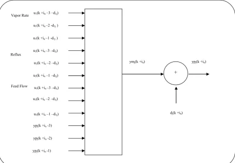
A combination of multiple neural networks is used to model a 3-input 2-output nonlinear dynamic system. As shown in Fig. 1, the proposed system consists of a two-dimensional array of neural network blocks. Each block consists of a one-step-ahead predictive neural model, NNj, which is identified to represent each output yj of the
MIMO system. Therefore, each block represents a multiple-input single-output (MISO) subsection of the whole MIMO system. All blocks in the j-th row utilize the same model as NNj. These models are employed to
predict the future outputs of the output yj over the
prediction horizon of P time steps.
The neural models are multi-layer feed-forward neural networks containing one hidden layer. The hidden layer contains 10 neurons. The activation function used for the neurons in the hidden layer is a Hyperbolic
Tangent function. A linear activation function is used for the single output node of each network. Fig. 2 shows the details of a typical NN block used in this system. As shown in this figure, past and current samples of each process input ui, and past and current output samples of
the process output yj are used as inputs to the network.
At time k, the input vector to the block NNj( in) is
defined as: ), d -3 -i (k u [ 1) -i (k
Ij n 1 n 1j (1) ), d -1 -i (k u ), d -2 -i (k
u1 n 1j 1 n 1j
), d -2 -i (k u ), d -3 -i (k
u2 n 2j 2 n 2j
), d -3 -i (k u ), d -1 -i (k
u2 n 2j 3 n 3j
), d -1 -i (k u ), d -2 -i (k
u3 n 3j 3 n 3j
, 1)] -i (k yp 2), -i (k yp 3), -i (k
ypj n j n j n T
Where ypj = yj is the j-th measured output of the plant,
dij is the time delay between the i-th input and j-th output
and T is the transpose operator. The future outputs in this vector are supplied by the preceding blocks.
A correction term dj is added to the model output ymj
to obtain the predicted output ypj. The correction term dj
accounts for the difference between the measured plant output and the model output. Each predicted disturbance dj(k + in) for any future time k + in is assumed to be
equal to the present dj(k).
At time k, the in-th predicted output vector is given
by: ... ), 1) -i (k I ( NN [ ) i (k
yp n 1 1 n (2) NNj(Ij(kin-1)),...NNN(IN(kin-1))]T
Where NNj is the j-th output neural network mapping,
and yp(k+in) = [yp1(k+in),… ypj(k+in),… ypN(k+in)]T.
Fig. 1: Two-dimensional array of neural network blocks
Fig. 2: A typical NN block
NN1(in)
NNN(in)
I1(k+in-1)
IN(k+in-1)
Ij(k+in-1)
NNj(in)
I1(k+P-1)
IN(k+P-1)
NN1(P)
NNN(P)
NNj(P)
NN1(1)
NNN(1)
NNj(1)
I1(k)
IN(k)
Ij(k)
ypj(k +in)
Feed Flow
dj(k +in)
ymj(k +in)
+
u1(k +in –2 -d1j )
u1(k +in –1 -d1j )
u1(k +in –3 –d1j)
u2(k +in –3 –d2j)
u2(k +in –1 –d2j)
u2(k +in –2 –d2j)
ypj(k +in -3)
ypj(k +in -2)
ypj(k +in -1)
u3(k +in –3 –d3j)
u3(k +in –1 –d3j)
u3(k +in –2 –d3j)
Reflux Vapor Rate
An attempt was made to identify and use a large one-step-ahead predictor for the MIMO process at each prediction step. However, finding such a large model required further training time and effort. In addition, it was not possible to complete the training to a reasonably small error. The errors for the one-step-ahead MIMO predictors are found to be greater than 0.5. Training iterations are greater than 10000.
Similar results were obtained by using a large P-step-ahead predictor fortheMIMOprocess.These observations may be explained as follows:
(a) The input vector to the MIMO model must contain all the measured outputs, whereas the input vector to the MISO model includes only one measured output.
(b) As shown in equations (1) and (2), each output of the network is related to an input vector. Each input vector generally consists of a distinctive set of pure lags between the network inputs and the output. Therefore, it is not possible to factorize the time lags in a single-step-ahead MIMO predictor.Consequently,we need to employ a long chain of past input samples in the input vector. This largely increases the network weights. Furthermore, the network attempts to approximate the underlying high-order dynamic relationships associated with pure lags. In addition, some of the input samples in this chain are not required to predict certain outputs. For example, if an output has a pure time delay of five sampling times with respect to an input, the current value of this input together with its past four input samples are not needed to determine the underlying relationship, as defined by equations (1) and (2), between the output and input.
Therefore, due to the reduced input and output data dimensionalities in the MISO model and reasonably low-order tight correlations between its inputs and the single output, the resulting model is more accurate. As a result, a combination of MISO models outperforms a single MIMO model.
NONLINEAR OPTIMIZATION
At time k, the task of the nonlinear optimizer is to calculate the present and future control actions which minimize the performance index:
N 1 j n P d 1 ij(k i )
-yp [ E ij n (3)
ydj(k in )]2 /2,
Where yp j(k + in ), in = 1+dij ,…, P and ydj(k + in ),
in = 1+dij ,…, P are the predicted and desired trajectories,
respectively of the j-th controlled variable.
At the current time, the i-th present and future manipulated inputsui(k - dij + in-1), in = dij +1,… dij +M;
dij +M P are calculated repeatedly as:
ui k
new
ui
k
old
E/ui
k
, (4)Where k’ is defined as k’ = k - d
ij + in-1, and is the
step size of the steepest descent method.
According to equation (3), the gradients of the objective function with respect to the manipulated variables can be obtained as:
N 1 j P d 1 i n j n j i ij n )] i k ( yd ) i k ( yp [ ) K ( u /E (5)
[ypj(kin)/ui(k')].
It can be shown that the partial differential of the output ypj of the NN employed in this work with respect
to its i-th input ui can be given by:
H 1 i h 2 i j h ) i , j ( u /yp (6)
[1Ohid(ih))2]1(ih,i),
Where 1 and 2 are connection weights in the first
and second layers, respectively, Ohid(ih ) is the output of
the ih-th neuron in the hidden layer, and H is the number
of neurons in the hidden layer.
Equation (5) is computed by the partial differential chain operations applied to the multiple neural network system.
PROCESS DESCRIPTION AND THE RIGOROUS DYNAMIC MODEL
The column was controlled by a decentralized system employing single-loop controllers. The liquid level in the re-boiler is maintained by varying the bottom product flow rate. The control loops at the top were modified as follows. The reflux flow is controlled by a flow controller. A level controller maintains the liquid level in the reflux drum by manipulating the cooling water to the overhead condenser. The entire liquid distillate was fed back to the column as reflux. By using this control configuration, the flow rate of the liquid distillate was made equal to the reflux flow rate. In order to implement this control scheme, the algorithm for the partial condenser was modified. The partial condenser described in the above reference assumed either a specific heat flux or a condensate temperature, whereas the newly-developed algorithm assumes a precise output condensate flow rate. The condensate rate was chosen to be equal to the reflux rate at each sampling time.
In addition, the column dynamic simulation routines presented in the above reference were modified, and they were coded using the Microsoft Visual C++ programming
environment. The distillation column simulation reflected the nonlinear characteristics and interactive feature of a real process.
The control loops described so far is required for stable operation of the column. To achieve composition control, the MIMO control scheme developed in this study is used. The controlled process variables are the temperatures T2 and T9 on stages 2 and 9 respectively
(counting from the bottom). Using the column simulator discussed in this section, it is found that the tray temperature T9 gives a good indication of heavy component loss out of the top of the tower. In addition, the temperature changes in T2 are substantially large
when the bottom product purity varies.
The steady state values of T2 (T2s) and T9 (T9s) are
105.73 oC and 79.07 oC respectively. The manipulated
variables employed are the reflux flow (L) and the steam valve stem position (V). The steady state values of L (Ls) and V (Vs) are 13 moles/min and 70% respectively. Changes in the feed flow rate (F) are employed as uncontrolled disturbances which tend to drive the controlled variables away from their set points. These changes are considered to be ‘measured’, that is, their effect is fed forward in control calculations. The steady state value of F (Fs) is 25 moles/min.
PROCESS NONLINEARITIES
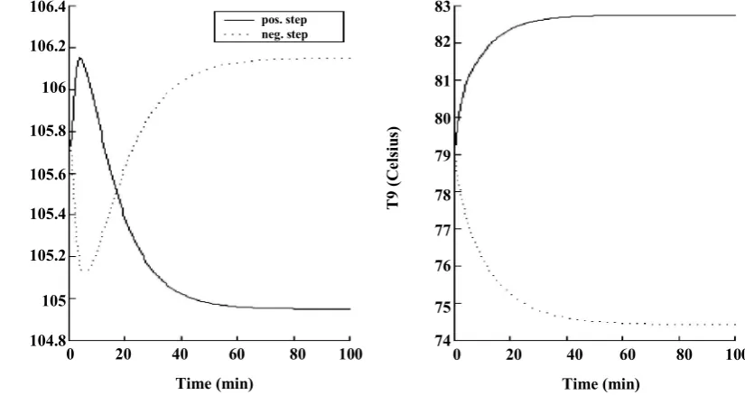
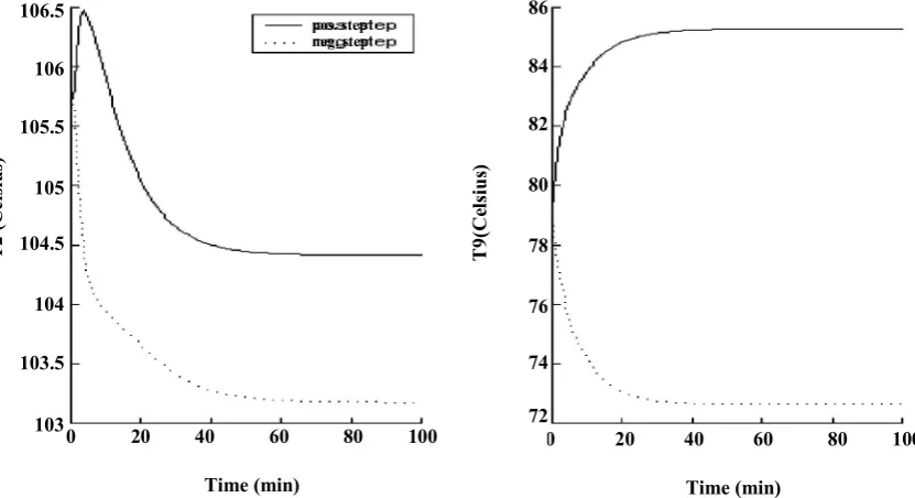
Open-loop temperature responses to step changes in the feed flow (F) are shown in Figs. 3-6. In Figs. 3, 4, 5 and 6 the step sizes are 5% and 10%, 15% and 20% of the steady-state value, respectively. From these figures, it can be seen that the temperature responses to equal positive and negative changes in the feed flow are not symmetrical.
The new steady-state values of the tray temperatures in Figures 3-6 are summarized in table 1. In addition, in this table T1 and T2 are deviations of the tray
temperatures from their corresponding initial operating points. Note that the tabulated values in the ninth column of this table indicate that T2 experiences a sign change
as the magnitude of the step change is altered from –10% to –15% of the steady-state value.
Therefore, the system exhibits dynamic and static nonlinear behavior in the region of operation.
MODELING BY PROCESS IDENTIFICATION
Linear model of the multi-component distillation column
Three dynamic response experiments were carried out in open loop to generate data for constructing the linear dynamic model of the multi-component distillation column. The experiments consisted of manipulating a single input at a time. The other inputs were set at a level indicated by the process condition.
In developing a linear model, one of the inputs was superimposed by a PRBS signal while the other two inputs were kept constant at their steady-state operating conditions. The PRBS sequence length was chosen to be 256 and the pulses had a duration time of 0.5 minutes. Values of inputs and control outputs would be recorded at discrete times. Deviations from the corresponding inputs and outputs steady-state values were used as the identification data to develop the model. In this work, the linear model was determined by extracting the step response data of the plant using the system identification toolbox of the MATLAB software.
Neural model of the multi-component distillation column
Table 1: The new steady-state values of the tray temperatures
F T2 T9 T2 T9 F T2 T9 T2 T9
0 105.73 79.07 0 0 0 105.73 79.07 0 0
5 105.33 81.07 -0.4 2 -5 106.10 76.78 0.37 -2.3 10 104.98 82.73 -0.75 3.66 -10 106.1 74.52 0.37 -4.55 15 104.69 84.11 -1.04 5.04 -15 105.16 73.16 -0.58 -5.91 20 104.45 85.27 -1.28 6.20 -20 103.22 72.63 -2.51 -6.44
Fig. 3: Open-loop temperature responses to 5% step changes in the feed flow
Fig. 4: Open-loop temperature responses to 10% step changes in the feed flow
T2 (C
elsiu
s)
106.3
106.2
106.1
106
105.9
105.8
105.7
105.6
105.5
105.4
105.3
0 20 40 60 80 100
Time (min)
0 20 40 60 80 100
Time (min)
pos. step neg. step
81.5
81
80.5
80
79.5
79
78.5
78
77.5
77
76.5
T9 (C
elsiu
s)
T9 (
C
elsiu
s)
T2 (C
elsiu
s)
0 20 40 60 80 100
Time (min)
0 20 40 60 80 100
Time (min) 83
82
81
80
79
78
77
76
75
74 106.4
106.2
106
105.8
105.6
105.4
105.2
105
104.8
pos. step neg. step
T2 (
C
elsiu
s)
T2 (C
elsiu
s)
T9 (C
elsiu
Table 2: Performance-index values of the controllers based on the linear and neural models of the column
M ISE(LM) ISE(NM) IAE(LM) IAE(NM) ITAE(LM) ITAE(NM) 4 5.0277 0.0263 12.2937 1.6779 600.7990 55.5436 3 5.1106 0.0328 12.3240 2.0356 600.9236 69.8976 2 5.3433 0.1996 12.9279 3.5162 639.6471 124.4246
1 11.4757 2.1960 25.2308 17.6019 1035.6478 629.7830
Fig. 5: Open-loop temperature responses to 15% step changes in the feed flow
Fig. 6: Open-loop temperature responses to 20% step changes in the feed flow
T
2
(C
elsiu
s)
0 20 40 60 80 100
Time (min)
0 20 40 60 80 100
Time (min) 106.5
106
105.5
105
104.5
104
103.5
103
86
84
82
80
78
76
74
72
T9(Ce
lsius
)
pos. step neg. step
T2 (C
elsiu
s)
0 20 40 60 80 100
Time (min)
0 20 40 60 80 100
Time (min) 106.4
106.2
106
105.8
105.6
105.4
105.2
105
104.8
104.6
pos. step neg. step
86
84
82
80
78
76
74
72
T
9
(Ce
lsius
)
T
2
(Ce
lsius
In addition, the column exhibits a nonlinear dynamic behavior.
If an excitation signal is applied at the operating point of the plant to extract its system dynamic and static characteristics, the results are not representative of the static and dynamic characteristics of the process over the entire range of the input variations. Due to the process nonlinearities, these results will be different if other operating conditions or different magnitudes of the excitation signal are implemented.
To capture the process nonlinearities, the tests were run over a wide range of operating conditions, i.e. different reflux flow rate (L), vapor flow rate (V) and the feed flow rate (F). The training was carried out around five samples of operating points on each of the intervals [(Ls-22.3%), (Ls+22.3%)], [(Vs-15.2%), (Vs+15.2%)] and [(Fs-20%), (Fs+20%)], for the variables L, V and F respectively.
At each operating point, a PRBS signal was used to persistently excite each input of the process. The PRBS sequence length was chosen to be 255 for the two manipulated variables L, V and F. The PRBS switching time was chosen to be 0.5 minutes. To avoid actuator restrictions, the magnitude of the PRBS at each input is set equally to its corresponding input amplitude span divided by 10.
RESULTS
MPC using the linear model of the column
Using the step-response data generated in the former section, a predictive controller is designed for the plant. This controller is based on the unconstrained form of the MIMO dynamic matrix control (DMC) law. Details of the derivation of this control algorithm are available in the literature [8].
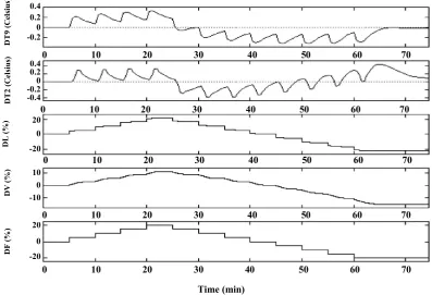
The controller based on the linear model of the column was applied to the plant. The distillation column was then subjected to changes in the feed flow rate (DF) using the multi-level signal as shown in Figs. 7 and 8. These changes take place within the interval of –20% to +20% of the operating feed flow rate. The magnitude of the quantum jump (step size) between one level and the next is equal to 5% of the steady-state value.
In Figs. 7 and 8, measured disturbances in the feed flow (DF), the controlled outputs (DT9 and DT2) and the profiles of the manipulated variables (DL and DV) are
shown. Each input or output value in these figures is shown using the deviation from its corresponding initial operating point (e.g. DL = L-Ls). For control calculations, P is fixed at four and the value of M is varied from 1 to 4. Profiles corresponding to M = 2 and M = 3 are not shown.
The control quality is evaluated by computing the performance criteria for different values of the control horizon M. All the three optimization criteria: ITAE, IAE and ISE are tried. The second, fourth and sixth columns of table 2 contain the values of the performance indices for the MPC systems based on the linear model (LM) of the plant. Referring to these values, one can see that the controller with the value of M = 4 has a superior performance. However, in real control, high value of M can yield more dynamic actions and stability problems can arise. Therefore, a lower value must be chosen for M.
MPC using the neural model of the column
The optimizer developed in the corresponding section was applied to control the column. The model role in the nonlinear MPC algorithm was satisfied by the multiple neural network model described in the related section. At the same time, the first principle model developed in associated section performs the column simulator role.
A similar sequence of changes in the feed flow rate as in the preceding section was made. The results are shown in Figs. 9 and 10. Each controlled output profile in Figs. 7 and 8 is compared to its corresponding profile in Figs. 9 and 10. The consequential assessment reveals that the MPC using the neural model rejects the disturbance much better than does the MPC using the linear model.
The third, fifth and seventh columns of Table 2 contain the values of the performance indices for the MPC systems based on the neural model (NM) of the plant. A comparison of the corresponding performance-index values in each row of this table shows that the response obtained with the MPC algorithm using the neural model is superior to that obtained using the linear model.
CONCLUSIONS
Fig. 7: Profiles of the controlled outputs (DT9 and DT2) and manipulated inputs (DL and DV) for regulatory control using MPC (P=4 and M=4) with a linear model of the column after measured disturbances in the feed flow rate (DF)
Fig. 8: Same as Fig. 7, but M=1
0 10 20 30 40 50 60 70
Time (min) 0 10 20 30 40 50 60 70
0 10 20 30 40 50 60 70
0 10 20 30 40 50 60 70
0 10 20 30 40 50 60 70
0.4 0.2 0 -0.2 0.4 0.2 0 -0.2 -0.4 20 0 -20 10 0 -10 20 0 -20 DT9 (C el sius) DT2 (C el sius) DL (%) DV ( %) DF (% ) Time (min) 0 10 20 30 40 50 60 70
0 10 20 30 40 50 60 70
0 10 20 30 40 50 60 70
0 10 20 30 40 50 60 70
0 10 20 30 40 50 60 70
0.2 0 -0.2
0.2 0 -0.2
20 0 -20
10 0 -10
20 0 -20
DT9
(C
el
sius)
DT2
(C
el
sius)
DL (%)
DV
(
%)
DF (%
Fig. 9: Profiles of the controlled outputs (DT9 and DT2) and manipulated inputs (DL and DV) for regulatory control using MPC (P=4 and M=4) with a neural model of the column after measured disturbances in the feed flow rate (DF)
Fig. 10: Same as Figure 9, but M=1
0 10 20 30 40 50 60 70
Time (min) 0 10 20 30 40 50 60 70
0 10 20 30 40 50 60 70
0 10 20 30 40 50 60 70
0 10 20 30 40 50 60 70
0.05 0 -0.05 -0.1 0.2 0 -0.2 20 0 -20 10 0 -10 20 0 -20 DT9 (C el sius) DT2 (C el sius) DL (%) DV ( %) DF (% ) 0 10 20 30 40 50 60 70
Time (min) 0 10 20 30 40 50 60 70
0 10 20 30 40 50 60 70
0 10 20 30 40 50 60 70
0 10 20 30 40 50 60 70
0.02
0 -0.02 0.04 0.02 0 -0.02 -0.04
20 0 -20
10 0 -10
20 0
-20
DT9
(C
el
sius)
DT2
(C
el
sius)
DL (%)
DV
(
%)
DF (%
derived in this paper provides excellent regulatory performance, as demonstrated for the multi-component distillation column. Simulation results demonstrate the ability of the proposed strategy to outperform the MPC algorithms based on the linear model of the plant.
Received: 3rd may 2003 ; Accepted: 22th December 2003
REFERENCES
[1] Billings, S.A. and Fakhouri, S.Y., Automatica, 18, 15 (1982).
[2] Leontardis, I. J. and Billings, S.A., Int. J. Contorl. 41, 303 (1985).
[3] Temeng, K. O., Schnelle, P.D. and McAvoy, T. J.,
Journal of Process Control, 5, 19 (1995).
[4] Lennox, B., Montague, G. A., Frith, A. M., Gent, G. and Beuan, V., Journal of Process Control, 11, 497 (2001).
[5] Duarte, M., Suarez, A. and Bassi, D., Powder Technology, 115, 193 (2001).
[6] Show, A. M. and Doyle, F. J., Journal of Process Control, 7, 255 (1997).
[7] Franks, R. G. E., John Wiley & Sons, “Modeling and Simulation in Chemical Engineering”, pp. 249-254 (1972).
[8] Garcia, C. E. and Morshedi, A. M., Cehm. Eng. Commun., 46, 073 (1986).