Equivalence and Minimization for Model Checking Labeled Markov Chains

(1)

Equivalence and Minimization for Model Checking Labeled

Markov Chains

Peter Buchholz

Informatik IV, TU Dortmund D-44221 Dortmund, Germany

Jan Kriege

Dimitri Scheftelowitsch

ABSTRACT

Model checking of Markov chains using logics like CSL or asCSL proves whether a logical formula holds for a state of the Markov chain. It has been developed in the last decade to a widely used approach to express performance and dependability quantities for models from a wide range of application areas. In this paper, model checking is extended to prove formulas for distributions rather than single states. This is a very natural way to express certain per-formance or dependability measures that depend on the state of the system rather than on a specific state in the state space of the Markov chain. It is shown that the mentioned logics can be eas-ily extended from states to distributions and model checking algo-rithms can also be easily adopted. Furthermore, new equivalences will be introduced that are weaker than bisimulation but still char-acterize the extended logics.

Categories and Subject Descriptors

G.3 [Probability and Statistics]: Markov Processes ; D.4.8 [Performance]: Stochastic Analysis

General Terms

Performance

Keywords

Model Checking, Labeled Markov Chains, Equivalence

1. INTRODUCTION

Model checking is nowadays widely used in functional and also in quantitative system analysis. The general idea is that one defines a property that a system should observe or should not observe as a formula in a temporal logic and then proves for each state or some states of the system, whether the formula holds or does not hold.

The mentioned approach is natural in functional system analysis where model checking is applied to the states of a labeled transi-tion system (LTS) or automaton and properties are defined in the temporal logic CTL [6]. Model checking can be applied in a fully

automated way after the LTS and the formula have been specified. The corresponding algorithms are efficient in terms of the size of the LTS which, however, may grow exponentially in terms of the system specification. The outcome of model checking is a clear decision which states fulfill the required property and which do not fulfill the property.

The situation is different if model checking is extended to quan-titative systems analysis as done with logics like CSL [1, 4, 3]. In this case, Markov chains with labeled states and possibly labeled transitions are considered. In contrast to functional properties two quantifications can be introduced. First, it can be required that a property has to hold within some time interval and it can be defined that a property holds at least or at most for a given probability. In this situation it is often not natural to prove whether the property or formula holds for a specific state since the state of a stochastic system is usually given as a probability distribution over the set of states. To give a simple abstract example, we consider some for-mula that should hold with a probability of at leastp. If we know that the system is with probabilityqin state 1 where the formula will hold with probabilityp1 <pand it is with probability (1−q)

in state 2 where the formula holds with probabilityp2>p, then the

formula holds if and only ifqp1+(1−q)p2≥p. This result cannot

be achieved with the known approaches where the outcome is that the formula holds in state 2 and does not hold in state 1. The use of distributions rather than states is natural in stochastic systems. Two typical examples are:

• One wants to check whether a formula holds in a specific situation, for example in steady state or after a specific event like a component failure, which cannot be characterized by a single state but by a probability distribution.

• The states of the Markov chain do not correspond to system states since phase type distributions are integrated to model non-exponential timing. In this case the system state corre-sponds to a set of states in the Markov chain and if one knows the time since the phase type distributions has been initiated, a probability distribution over the set of phases can be com-puted and it can be decided whether a formula holds for the distribution which means that it holds for the corresponding abstract system state.

Surprisingly, model checking has, to the best of our knowledge, not been extended to distributions. Distributions contain the common viewpoint of states, because a distribution assigning probability 1 to a single state corresponds to the proof that the state fulfills the formula. However, it is in general not possible to prove formulas that are defined for distributions using state formulas.

In this paper we extend the established logics CSL and asCSL [3] to consider distributions rather than states. This can be done in a

(2)

very natural way and allows one to easily adopt model checking algorithms. A side effect is that new equivalence relations can be defined that preserve logical formulas. It is known that for CSL over states stochastic bisimulation is the equivalence that charac-terizes the logic. However, if one considers CSL over distributions, a weaker relation can be defined which relates distributions and in-cludes the case that a state is related to a distribution over several states. The corresponding equivalence will be defined and it will be outlined that equivalence is still decidable and a minimal, possi-bly non-Markovian, representation can be computed for a Markov chain.

The outline of the paper is as follows. In the next section we briefly review related work. Then we introduce the basic model class, labeled Markov chains in continuous time. In Section 4 equivalence relations are defined and Section 5 introduces the ex-tended logics, presents basic steps for model checking and shows that equivalent Markov models are indistinguishable under the log-ical formulas. All proofs are given in the appendix. Some smaller examples are used as running examples and Section 6 contains re-sults for medium sized examples.

2. RELATED WORK

In the past labeled Markov processes have been defined in var-ious forms. These definitions include stochastic process algebras [17] whose underlying stochastic model can be interpreted as a Markov process, stochastic automata [24] and interactive Markov chains [16] to mention only a few examples. For those Markov processes model checking approaches have been defined as exten-sions to the classical model checking of labeled transition systems or automata [6].

Usually model checking means to prove for each state whether a formula holds or does not hold. For performance or dependabil-ity analysis where time-dependent properties have to be analyzed the model is extended by stochastic timing information resulting in CTMCs. Model checking CTMCs based on the logic CSL has been introduced in [1]. CSL has been extended in several ways, one ex-tension is asCSL [3] that supports transition labels, while CSL con-siders only state labels. Moreover, efficient algorithms have been developed to verify CSL formulas [4]. For more results in this area we refer the interested reader to the overview papers [5, 20].

To decrease the effort for the analysis of Markov chains in gen-eral and in particular for model checking often bisimulation is used to reduce the state space and to obtain a smaller but equivalent representation of the process. Bisimulation for untimed systems has been introduced in [23, 22] and was later extended to discrete time Markov chains in [21] and continuous time Markov chains in [8, 17]. The relation between CSL and bisimulation is derived in [2] and [18] presents several case studies that studied the effect of bisimulation on model checking. While the approaches for bisim-ulation mentioned so far all work at the state level, [13] extended bisimulation to the trace distribution of labeled Markov processes and [14] considers bisimulations if the initial state is given by a distribution rather than a single state. A model checking approach that extends CSL to models with phase type distributions is given in [9]. Finally, [12] presented transformations of Markovian and non-Markovian models that define general equivalence relations and al-low for an efficient minimization of those models.

3. LABELED MARKOV PROCESSES

We consider Markov chains with labeled transitions and states in continuous time following similar models that have been proposed

in the literature over more than two decades [8, 13, 15, 16, 17, 21, 24].

Definition1 (LabeledMarkov chains). A continuous time

la-beled Markov chain (CTLMC) is defined by the tuple

CM= S, ϕ,A,Ge(e∈ A),AP,L,

where

• S={s0, . . . ,sn−1}is a finite set of states,

• ϕ∈[0,1]1,n_{defines a probability distribution over S ,}

• Ais a finite alphabet of transition labels,

• Ge∈Rn≥,0nis for each e∈ Aan n×n transition rate matrix, • AP is a set of atomic propositions, and

• L:S→2AP_{is the state labeling function.}

We often identify states by their number, i.e.,imeanssiif the in-terpretation is clear from the context. Thus, Ge(i,j) is the rate of a transition from si to sj labeled withe. We assume that in every state transitions with label e are either enabled such that

Pn

j=1Ge(i,j) > 0 or disabled such thatPnj=1Ge(i,j) = 0. The model includes CTMCs with only state labels (i.e.,A = ∅). In this case we writeGrather thanGefor the transition matrix. Ob-serve that in contrast to most other definitions of labeled Markov models, the initial distribution is part of the definition. To define a unique initial statesi, vectorϕ=eiis used whereeiis a row vector with 1 in positioniand 0 elsewhere. CTLMCs can be completely described by vectors and matrices. Define fora∈APra ∈ {0,1}n,1 withra(i) =1 ifa∈ L(si) and 0 ifa <L(si). Sometimes we use Ra =diag(ra) which is an×ndiagonal matrix withra(i) in posi-tion (i,i). (ϕ,Ge(e∈ A),ra(a∈AP)) is a short hand notation for a CTLMC. Sometimes we skip the setsAandAP, if they are clear from the context or irrelevant.

Transitions in continuous time Markov chains take place after an exponentially distributed duration. An infinite path of a CTLMC is defined asσ =(s(0),e(0),t(0)),(s(1),e(1),t(1)), . . .wheres(h) ∈

S,e(h)∈ Aandt(h)∈_R≥0is the time between thehth andh+1th

transition or the time before the first transition ifh= 0. A finite path is given by

σ= (s(0),e(0),t(0)),(s(1),e(1),t(1)), . . . , (s(|σ| −1),e(|σ| −1),t(|σ| −1)),s(|σ|)).

σ(h)=(s(h),e(h),t(h)) forh<|σ|,s(h) forh=|σ|and undefined otherwise. σi

h for 0 ≤ h ≤ i ≤ |σ|is the subpath including the elementshthroughi.

LetG¯e=diag(Ge1) andI G¯ =Pe∈AG¯ebe the diagonal matrix of transition rates, then

Dens(σ)=

|σ|−1 Y

h=0

e−t(h)G¯(s(h),s(h))Ge(h)(s(h),s(h+1))

defines the value of the probability density for the pathσ.Ωiis the set of all paths of lengthiandΩis the set of all finite paths.

For the definition of equivalent behavior, events and/or state pro-positions are observed and not detailed states. Thus, a sequence ς=

(a0,e0,t0), . . . ,(a|ς|−1,e|ς|−1,t|ς|−1),a|ς|

whereah ∈AP,eh ∈ A andth ∈ R≥0 is a finite observable behavior. If for a CTLMCA

(3)

all finite observable behaviors. For a CTLMC and an observable behavior, the density is given by

Dens(ϕ,Ge,ra)(ς)=ϕ

        

|ς|−1 Y

h=0

Rahe

−thG¯_G

eh

        

ra|ς|.

Running Examples

Thefirst exampleis a CTLMC (ϕ,G,ra(a∈AP={a,b})) without transition labels where

G=

               

0 0 0 µ0

0 0 0 µ1

0 0 0 µ2

λ0 λ1 λ2 0                

,

statess0, . . . ,s2are labeled withaand states3is labeled withb.

4. EQUIVALENCE OF LABELED MARKOV

CHAINS

We first define equivalence of CTLMCs as a natural adoption of trace equivalence for labeled Markov processes [13].

Definition 2. Two CTLMCs(ϕ,Ge(e ∈ A),ra(a ∈ AP))and (υ,He(e∈ A),sa(a∈ AP))are equivalent if and only if∀ς ∈ Υ:

Dens(ϕ,Ge,ra)(ς)=Dens(υ,He,sa)(ς).

In the following we define different equivalences for CTLMCs ba-sed on the minimal non-Markovian representation of Markov mod-els developed in [12] and extended to compositional modmod-els in [10]. These general equivalence relations are extensions to bisimulation on distributions as defined in [14].

LetCM₁ =(ϕ,Ge(e∈ A),ra(a∈ AP)) andCM2 =(υ,He(e∈

A),sa(a∈AP)) be two CTLMCs withmandn<mstates, respec-tively. Then the following relations are defined:

1. CM1 ∼ CM2holds if and only if there exists a matrixV∈ Rm,nwithV1In=1Im, such thatϕV=υ,GV¯ =V ¯H,∀e∈ A: GeV=VHeand∀a∈AP:RaV=VSa.

2. CM1' CM2holds if and only if there exists a matrixW∈ Rn,mwithW1Im =1In, such thatϕ=Wυ,W ¯G =HW,¯ ∀e∈

A:WGe=HeWand∀a∈AP:WRa=SaW.

Ifm=na third relation is defined:

3. CM1 CM2holds if and only if there exists a matrixU∈ Rn,nwithU1I=1, such thatI ϕU=υ,GU¯ =U ¯H,∀e∈ A :

GeU=UHeand∀a∈AP:RaU=USa.

The first relation is a natural extension of strong lumpability [19] and bisimulation for labeled Markov chains [8, 16, 17]. For strong lumpability or bisimulation matrixVcontains only elements from

{0,1} which implies that in each row ofV exactly one element equals 1, the remaining elements are 0. Thus, strong lumpabili-ty and bisimulation describe a mapping where one state from the larger state space is mapped on exactly one element in the smaller state space. In the more general definition used here, a state in the larger state space is represented by a weighted sum of states from the smaller state space. In a similar way, the second equivalence can be related to weak lumpability of Markov chains [19]. For de-tails we refer to [11].

The following theorem shows that any of the above equations assures equivalence, a proof is given in the appendix.

Theorem 1. Two CTLMCsCM1andCM2that are in one of the

relations∼,'orare equivalent.

ζ,De,ra

∼

ζ(1)_,_D(1)

e ,r

(1)

a

∼

' _'

η(2)_,_F(2)

e ,s

(2)

a

η,Fe,sa

ζ(2)_,_D(2)

e ,r

(2)

a

η(1)_,_F(1)

e ,s

(1)

a

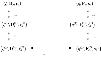
Figure 1: Relation≈for CTLMCs

From [12] it can be concluded thatUis non-singular and that the matricesVandWhave full rank, such that we can find a left- and right-inverse, respectively, i.e.V#_V₌_I_and_WW#₌_I.

Now, assume that two CTLMCs, (ζ,De,r) with mstates and (η,Fe,sa) withnstates are given. Then the two processes are in relation≈if the diagram in Figure 1 commutes. For each step in the diagram, an efficient algorithm exists that computes a minimal equivalent representation according to the required relation. Com-putation of the matricesVandWand the corresponding minimal representations can be done with the staircase algorithm from [12] with an effort inO(|A| ·m4_{) for CTLMCs of order}_m_{. Matrix}_U_can

be computed with an effort inO(|A| ·m3_{) for processes of order}_m

using algorithms for the solution of Sylvester equations [7]. The following corollary follows from Theorem 1.

Corollary 1. If two CTLMCs are in relation≈, then they are

equivalent.

Running Examples

For thefirst exampleassume thatµ0,µ1and letp=(µ2−µ1)/(µ0−

µ1). Then define matrices

V=

               

1 0 0

0 1 0

p 1−p 0

0 0 1

               

, H=

          

0 0 µ0

0 0 µ1

λ0+pλ2 λ1+(1−p)λ2 0           

and the CTLMC (υ=ϕV,H,sa(a∈ {a,b})). Assume that the last state is labeled withband the first two states are labeled witha. Then (υ=ϕV,H,sa(a∈ {a,b})) is in relation∼to (ϕ,G,ra). Ob-serve that the new process is a CTLMC if and only ifp ∈ [0,1].

5. MODEL CHECKING LABELED MARKOV

CHAINS

Different logics have been defined for model checking Markov chains with state and transition labels. Usually model checking means to prove for each state whether a formula holds or does not hold. This viewpoint has been transferred from qualitative system analysis to quantitative system analysis using transition probabili-ties or rates. However, if the state is defined in terms of a distri-bution rather than a unique state, as it is the case here and in [13], then a formula should hold with respect to a distribution which does not necessarily mean that it has to hold for all states with non-zero probabilities as shown below.

(4)

all cases we extend the logics to check a formula for a CTLMC with a given initial distribution. By defining an initial distribution equal toei, this includes the common case, where a formula is checked for statesi. We extend the two logics CSL and asCSL in the men-tioned way resulting in logics dCSL and dasCSL, where the letter d stands for distribution.

We begin withdCSLwhich is defined over CTLMCs without transition labels such thatCM=(µ,G,ra(a∈AP)).

Definition3 (dCSL). A dCSL formula is defined as Γ::= DS_Z_p(Φ)| DP_Z_p(Ψ)

whereZ∈ {≤,≥}, p∈[0,1], I⊂R≥0is some non-empty interval,Φ

is a state formula

Φ::=tt|a|Φ∧Φ| ¬Φ| S_Z_p(Φ)| P_Z_p(Ψ)

andΨis a path formula

Ψ::= ΦUIΦ|XIΦ.

The syntax and semantics of the state and path formulas is as in CSL [1, 4].

For a state distribution formulaΦand state s ∈ S, s |= Φor

s 6|= Φholds. Letr_Φbe a vector withr_Φ(i) = 1 ifsi |= Φand 0 otherwise. As beforeR_Φ = diag(rφ). Furthermore we define

for some transition matrix of a CTLMCGand a state formulaΦa matrixG[Φ] as the matrix that results fromGwhen all states where

Φdoes not hold are made absorbing. This means thatG[φ] (i•)= (0, . . . ,0) ifsi6|= ΦandG[φ] (i•)=G(i•) ifsi|= Φ1.

Then for some distributionµ,

µ|=DS_Zp(Φ) ⇔ µrΦZp. (1)

Forµ=ei,Z=≥andp=1,µ|=DSZp(Φ) is equivalent tosi|= Φ which shows that for any CSL formula an equivalent dCSL formula exists.

To handle path formulas we define in accordance to [4]γ(σ,h)=

t(h), the time spent between theh−1th andhth transition at path σanda@t = s(h) where Ph−1

j=1t(j) ≤ tand Ph

j=1t(j) > t. The

latter sum is, of course, only defined for paths of a length≥h. The following two sets are defined

Ωi(Φ1UIΦ2) = σ|s(0)=si∧ ∃t∈I:a@t|= Φ2∧

∀t0_<

t:a@t0_|_{= Φ1}

Ωi(XIΦ) =

_σ_|

s(1)|= Φ∧γ(σ,0)∈I

Under appropriate measurability conditions the probability of an arbitrary path fromΩi(·) is well defined (see [4]) and can be com-puted from the following equations

q_Φ₁U[t1,t2 ]_Φ₂ = e

t1(G[Φ1]−G¯[Φ1])_R

Φ1e

(t2−t1)(G[Φ1∧¬Φ2]−G¯[Φ1∧¬Φ2])_r

Φ2(2) fort1>0

q_Φ₁U[0,t2 ]Φ2 = e

t2(G[Φ1∧¬Φ2]−G¯[Φ1∧¬Φ2])_r

Φ2 fort1=0 (3) qX[t1,t2 ]Φ = e

−t1G¯

Z t2

t=t1

e−tG¯_Gr

Φdt

whereI =[t1,t2] with 0≤t1 ≤t2. Observe that for dCSL

transi-tions are not labeled such that we can writeGrather thanGe. The vectorsq_Φ₁U[t1,t2 ]_Φ₂andqXt₁Φcan be computed efficiently using

uni-formization as shown in [4].

1_{Observe that the definition of}_G[_Φ_{] corresponds to}_G[_¬_Φ_{] in}

[4] such that the equations syntactically differ but have the same semantics.

Distributionµobserves the distributional path formulas, if the following equations hold.

µq_Φ

1U[t1,t2 ]Φ2Zp ⇔ µ|=DPZp

Φ1U[t1,t2]_Φ2

µqX[t1,t2 ]ΦZp ⇔ µ|=DPZp

Xt1Φ

Observe that the major effort to verifyµ|=DP_Z_p(. . .) is required to compute the vectorsq. in (2,3). After the vectors are available

at most one inner product has to be computed. This means that the asymptotic effort to verify dCSL formulas is the same than the effort to verify CSL formulas.

The following theorem shows the relation between≈and dCSL formulas, the proof can be found in the appendix.

Theorem 2. LetCM1 =(ϕ,G,ra(a∈ A))andCM2 =(υ,H,

sa(a∈ A))be two CTLMCs withCM1≈ CM2, then for any dCSL

formulaΓ:

ϕ|= Γ ⇔ υ|= Γ.

Finally, we consider the extension of asCSL todasCSLwhich fol-lows the same ideas used for the definition of dCSL.

Definition4 (dasCSL). A dasCSL formula is defined as Γ::=DS_Zp(Φ)| DPZp(Ψ)

whereZ∈ {≤,≥}, p∈[0,1], I⊂_R≥0is some non-empty interval,Φ

is a state formula

Φ::= tt|a|Φ∧Φ| ¬Φ| S_Zp(Φ)| PZp(Ψ)

andΨis a path formula

Ψ::=αI

which is formally defined below.

For the definition of path formulas we follow [3]. αis a program that specifies properties which have to hold for finite paths. Pro-grams are specified by the following grammar

α::= ε|(Φ,e)|α;α|α∪α|α∗

whereΦis a dasCSL state formula ande∈ A ∪ {√},√is a symbol that does not belong toA. We defineα0 =εandαi =α;αi−1for

i ≥ 1. Symbol ; denotes the concatenation of two programs and α∗

the Kleene star, the n-fold sequential composition for arbitrary

n>0.

The set of pathsΩ(α) that fulfill the programαcan be defined inductively from the following sets of finite paths

Ω(ε) = σ_{| |}σ_|=

0

Ω(Φ,e) = σ_|

s(0)|= Φ∧e(0)=e

Ω(Φ,√) = _σ_|

s(0)|= Φ∧ |σ|=0

Ω(α1;α2) = σ| ∃h∈ {0,1, . . . ,|σ| −1}:

σh

0∈Ω(α1)∧σ

|σ|

h ∈Ω(α2) o

Ω(α1∪α2) = σ|σ∈Ω(α1)∪Ω(α2) Ω(α∗

) = σ_{| ∃}

h≥0 :σ∈Ω(αh)

A pathσbelongs to the setΩ(αI_{), if}_σ_∈_Ω₍_α_{) and}P|σ|−1

h=0 t(h)∈I.

Since programs are regular expressions they can be equivalently characterized as the language of a finite acceptor. This acceptor can be transformed into a deterministic acceptor which means that for each pathσ, there exists a unique run of the acceptor and the path is accepted if it ends in a final state. Details of the construction of the acceptor for a programαand a CTLMCCMcan be found in [3].

For some programαand CTLMCCMletDA=(Z,B, δ,z0,F)

(5)

• Zis a finite set of states,

• Bis an alphabet of transition labels of the form (Φ,e) where

Φis a state formula forCMande∈ A,

• δ:Z× B →Zis the (deterministic) transition function,

• z0∈Zis the unique initial state, • F ⊂Zis the set of final states,

be a deterministic automaton that accepts exactly the paths ofCM

that result in a successful run of programα. Observe that√does not appear as transition inscription here. The generation of the de-terministic automaton including the elimination of√is described in [3].

To check µ |= DP_Zp

αI

, we build the composed automaton

DA × CMCM= S, ϕ,A,Ga,AP,L

without transition labels which can be interpreted as a CTLMC without transition labels. We build the automaton on the complete state spaceZ×Swhich might contain unreachable states and is not necessary for model checking but helps to prove the preservation of formulas by the previously proposed equivalence relations.

The composed automaton is

CM0=DA × CM= Z×S, υ,∅,F,AP0,L0

where

• υ= ϕ,0, . . . ,0

,

• F is a matrix of order|Z| · |S| × |Z| · |S|which is built by

|Z| × |Z| submatricesFz,z0 of order |S| × |S|where F_z_,_z0 =

P

(Φ,e):δ(Φ,e)=z0RΦGe,

• AP0₌

AP∪ {f in}withf in<AP,

• L0

(z,s)=

(

L(s) ifz<F,

L(s)∪ {f in} ifz∈ F.

Then model checking can be performed using standard methods for the new CTLMC. Letrf inbe a vector with 1 in positioniif

si=(s,z),z∈ F and 0 otherwise. IfI=[0,t], then vector qαI =et(F[¬f in]−F¯[¬f in])rf in (4) is computed by a transient analysis and

ϕ|=DP_Zp

αI

⇔ υqαI Zp. (5)

ForI=[t1,t2] with 0<t1≤t2, vectorqαIis computed in two steps

which are explained in [3]. We first compute the vector

ˆ

qαI =e(t2−t1)(F[¬f in]−F¯[¬f in])rf in (6) by a transient analysis. This corresponds to the second step de-scribed in [3]. Then

qαI =et1(F−

¯ F)_q_ˆ

αI (7)

is computed and used in (5) to check the formula. Again the asymp-totic effort to check a dasCSL formula for distributionµis the same than the effort to check the same formula in asCSL for a single state because the evaluation of (6) and (7) requires much more time than the computation of the final result by an inner product (dasCSL) or by selecting a single element (asCSL).

Theorem 3. LetCM1 =(ϕ,G,ra(a∈ A))andCM2 =(υ,H,

sa(a ∈ A)) be two CTLMCs withCM1 ≈ CM2, then, for any

dasCSL formulaΓ:

ϕ|= Γ ⇔ υ|= Γ.

The proof can be found in the appendix.

6. EXAMPLES

6.1 An M/M/1 Queue

We consider a simple M/M/1 queue with capacity 5 as a running example to present dasCSL model checking. Arrivals occur with rateλ =1, the service rate isµ =2. The CTLMC corresponding to the system is shown in Fig. 2. We use two transition labelsa

and b. ais used for normal transitions where either a customer arrives or is served,bis used for customers that are lost due to a full queue. The atomic propositionemptyis associated with state

s0. The other states are labeled withbusy. We analyze the system

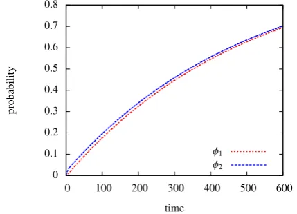
for two different scenarios regarding the initial distribution of the queue length. The distributionµ1 =[0.4,0.3,0.2,0.1,0,0] models

a normal load, while distributionµ2=[0.1,0.15,0.2,0.3,0.15,0.1]

models a high load.

Then, dasCSL is used to investigate the probability that at most 2 customers are lost before theemptystate is reached again within the nextttime units. The deterministic automaton describing the

q0 q1 q2 q3

empty,a

busy,a

·,b

busy,a

empty,·

·,b

busy,a

empty,·

·,b

·

Figure 3: Deterministic Automaton

mentioned property is shown in Fig. 3. It accepts inputs that vio-late the property mentioned above, i.e. sequences with more than two blocked customers before theemptystate is reached. The com-posed automaton has a 24×24 matrixF. The submatrices are given byFq0,q0 = Ga,Fq0,q1 = Fq1,q2 = Fq2,q3 =Gb,Fq1,q0 =Fq2,q0 = RemptyGa,Fq1,q1=Fq2,q2=RbusyGaandFq3,q3=Ga+Gb. All other submatrices are zero. With these matrices we evaluated Eq. 4 for different values fortbetween 0 to 600. The probabilitiespfor that µi|=DP≤p

α[0,t]

is fulfilled are shown in Fig. 4.

0 0.1 0.2 0.3 0.4 0.5 0.6 0.7 0.8

0 100 200 300 400 500 600

probability

time φ1

φ2

Figure 4: Results for the Queueing Example

6.2 A PH/PH/1 Queue

(6)

s0 s1 s2 s3 s4 s5

λ,a

µ,a

λ,a

µ,a

λ,a

µ,a

λ,a

µ,a

λ,a

µ,a

λ,b

Figure 2: CTLMC of Queueing example

coefficient of variation 10). For the service time distribution we choose a 2-phase hyperexponential distribution with initial state vector (0.97559,0.024405) and phase rates (1.99512,0.04881) (i.e., a distribution with mean 1 and squared coefficient of variation of 20). The queue has a maximal capacity of 10 and we add an ad-ditional absorbing state that is entered, if a customer arrives to a fully occupied queue. States can be described by a triple (i,j,k) wherei∈ {−1,0, . . . ,10}. i=−1 defines the absorbing state, and

i= 0, . . . ,10 describes the number of customers in the queue. j

indicates the phase of the hyperexponential distribution for the ar-rivals and becomes 0 fori=−1. Similarly,kindicates the phase of the hyperexponential distribution for the service and becomes 0 for

i=−1 andi=0. Thus, the state space consists of 43 states, 2 states where the queue is empty, 40 states with 1 through 10 customers in the queue and one absorbing state indicating an overflow. We assume that the two states describing the empty queue observe an atomic propositionemptyand the absorbing state observes atomic propositionfull. Transitions are not labeled.

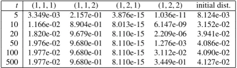
t (1,1,1) (1,1,2) (1,2,1) (1,2,2) initial dist. 5 3.349e-03 2.157e-01 3.876e-15 1.036e-11 8.124e-03 10 1.166e-02 8.904e-01 8.013e-15 6.147e-09 3.152e-02 20 1.820e-02 9.679e-01 8.110e-15 2.209e-06 3.941e-02 50 1.976e-02 9.680e-01 8.110e-15 1.276e-03 4.086e-02 100 1.977e-02 9.680e-01 8.110e-15 3.112e-02 4.090e-02 500 1.977e-02 9.680e-01 8.110e-15 3.449e-01 4.127e-02

Table 1: Value ofpfor whichDP>p

¬emptyU[0,t]_{f ull}_{holds for}

the PH/PH/1 queue.

The goal is now to computeDP>p

¬emptyU[0,t]_{f ull}_which

equals the probability that a customer is lost before the system be-comes empty. We assume that the analysis begins immediately af-ter the first customer arrived to an empty system. Thus, the system can be in one of four states (1,1,1), (1,1,2), (1,2,1) and (1,2,2). This implies that the initial distribution can be easily computed from the two initial vectors of the hyperexponential distributions. Naturally, this defines a distribution and not a single state. Table 1 shows the probabilitiespfor which the formula holds for different values oft, for the initial distribution and for the different states in which the system can be in for population 1. Obviously,pdepends heavily on the state and model checking of the isolated states does not answer the question whether the formula holds for the system or does not hold. Whereas it holds with some probability between the extreme values for the states when the distribution is considered. Standard CSL cannot be used to express the required property.

6.3 The Workstation Cluster

The workstation cluster is a widely used benchmark in stochastic model checking [18]. The model describes two clusters of worksta-tions connected via a backbone net and each cluster itself is realized by a star topology with a central switch andNworkstations. The system providespremiumservice as long as at leastNconnected workstations are available andminimumservice if at leastdN/2e

connected workstations are available. We assume that states are

la-beled withminif they provideminimumbut notpremiumservice, they are labeled withpremif they providepremium service. As shown in [18] stochastic bisimulation can be applied to reduce the state space of the model by a factor of approximately two, a fur-ther reduction with the equivalence relation presented here is not possible.

A typical formula for the analysis of the workstation cluster is

DS≥p

minU[0,t]_prem

which states that the system delivers min-imumservice and recovers withintunits of time to a state where

premium service is provided without reaching a state where the service level drops below minimum. Typically one would like to analyze the formula starting from the point where the service drops frompremiumtominimum.

The formula can be checked forCM= S, ϕ,∅,G,{min, prem, none},L

whereG−G¯ is the generator matrix of the CTMC de-scribed by the workstation cluster. Letϕ¯(G−G)¯ =0be the sta-tionary vector of the CTMC which is for the example unique since the CTMC is ergodic. Then the initial vector for the mentioned situation is computed as

ϕ(i)=

        

0 ifmin<L(si) P

j:prem∈L(s j)ϕ(¯j)G(j,i) P

k:prem∈L(sk)Pl:min∈L(sl)ϕ(¯k)G(k.l) ifmin∈L(si)

Then the until formula can be evaluated as described above.

7. CONCLUSIONS

We presented an extended approach for model checking Markov models with labeled transitions and states. In contrast to known approaches, distributions rather than single states are considered. It is shown that common logics can be easily extended to adopt this viewpoint and that the approach allows one to extend equivalence relations that preserve logical formulas beyond bisimulation. The use of distributions can be applied to prove properties of a system that hold after specific events that have been observed but do not necessarily imply that the system is in a specific state. Examples are arrivals or departures of customers, failure of components or even the steady state distribution conditioned on some subset of the state space. It is quite natural to ask whether a system fulfills a formula in such a situation which is possible with the extended log-ics proposed here but cannot be analyzed with standard approaches for model checking. Standard model checking algorithms can be easily adopted for the extended logics whereas the introduction of the new equivalence relations is a real extension of bisimulation at state level since bisimulation no longer characterizes the smallest system that is indistinguishable under a formula. The latter aspect will be investigated in the future.

(7)

8. REFERENCES

[1] A. Aziz, K. Sanwal, V. Singhal, and R. Brayton. Model checking continuous time Markov chains.ACM Trans. on Computational Logic, 1(1):162–170, 2000.

[2] A. Aziz, V. Singhal, and F. Balarin. It usually works: The temporal logic of stochastic systems. In P. Wolper, editor,

CAV, volume 939 ofLecture Notes in Computer Science, pages 155–165. Springer, 1995.

[3] C. Baier, L. Cloth, B. Haverkort, M. Kuntz, and M. Siegle. Model checking Markov chains with actions and state labels.

IEEE Transactions on Software Engineering, 33(4):209–224, 2007.

[4] C. Baier, B. Haverkort, H. Hermanns, and J.-P. Katoen. Model checking algorithms for continuous time Markov chains.IEEE Transactions on Software Engineering, 29(7):524–541, 2003.

[5] C. Baier, B. Haverkort, H. Hermanns, and J.-P. Katoen. Performance evaluation and model checking join forces.

Comm. ACM, 53(9):76–85, 2010.

[6] C. Baier and J.-P. Katoen.Principles of Model Checking. MIT Press, 2008.

[7] R. H. Bartels and G. W. Stewart. Solution of the matrix equation AX+XB=C.Comm. ACM, 15:820–826, 1972. [8] P. Buchholz. Markovian process algebra: composition and

equivalence. In U. Herzog and M. Rettelbach, editors,Proc. of the 2nd Work. on Process Algebras and Performance Modelling, pages 11–30. Arbeitsberichte des IMMD, University of Erlangen, no. 27, 1994.

[9] P. Buchholz, J. Kriege, and D. Scheftelowitsch. Model checking stochastic automata for dependability and performance measures. InDSN, 2014.

[10] P. Buchholz and M. Telek. Composition and equivalence of Markovian and non-Markovian models. InQEST, pages 213–222. IEEE Computer Society, 2011.

[11] P. Buchholz and M. Telek. Rational processes related to communicating Markov processes.J. Appl. Probab., 49(1):40–59, 2012.

[12] P. Buchholz and M. Telek. On minimal representations of rational arrival processes.Annals OR, 202(1):35–58, 2013. [13] L. Doyen, T. A. Henzinger, and J.-F. Raskin. Equivalence of

labeled Markov chains.Int. J. Found. Comput. Sci., 19(3):549–563, 2008.

[14] C. Eisentraut, H. Hermanns, J. Krämer, A. Turrini, and L. Zhang. Deciding bisimilarities on distributions. In

Quantitative Evaluation of Systems - 10th International Conference, QEST, volume 8054 ofLecture Notes in Computer Science, pages 72–88. Springer, 2013.

[15] H. Hansson and B. Jonsson. A logic for reasoning about time and reliability.Formal Aspects of Computing, 6:512–535, 1994.

[16] H. Hermanns.Interactive Markov Chains: The Quest for Quantified Quality, volume 2428 ofLecture Notes in Computer Science. Springer, 2002.

[17] J. Hillston. A compositional approach for performance modelling. Phd thesis, University of Edinburgh, Dep. of Comp. Sc., 1994.

[18] J.-P. Katoen, T. Kemna, I. S. Zapreev, and D. N. Jansen. Bisimulation minimisation mostly speeds up probabilistic model checking. In O. Grumberg and M. Huth, editors,

TACAS, volume 4424 ofLecture Notes in Computer Science, pages 87–101. Springer, 2007.

[19] J. G. Kemeny and J. L. Snell.Finite Markov chains. University series in undergraduate mathematics. VanNostrand, New York, repr edition, 1969.

[20] M. Z. Kwiatkowska, G. Norman, and D. Parker. Stochastic model checking. In M. Bernardo and J. Hillston, editors,

SFM, volume 4486 ofLecture Notes in Computer Science, pages 220–270, 2007.

[21] K. Larsen and A. Skou. Bisimulation through probabilistic testing.Information and Computation, 94:1–28, 1991. [22] R. Milner.Communication and concurrency. Prentice Hall,

1989.

[23] D. Park. Concurrency and automata on infinite sequences. In

Proc. 5th GI Conference on Theoretical Computer Science, pages 167–183. Springer, 1981.

[24] B. Plateau. On the stochastic structure of parallelism and synchronisation models for distributed algorithms.ACM Performance Evaluation Review, 13:142–154, 1985.

APPENDIX

Proof of Theorem 1

We show the proof for relation∼. LetCM1=(µ,Ge(e∈ A),ra(a∈

AP)) of ordermandCM2=(ψ,He(e∈ A),sa(a∈AP)) of ordern be in relationCM1∼ CM2. Then

RaGeV=RaVHe=VSaHe

for alla∈ AP, alle∈ A. Observe thatRaV=VSaimpliesra = Vsasince

RaV1I=Ra1I=raandRaV1I=VSa1I=Vsa.

Observe that

etG¯_V ₌ P∞

h=0

tG¯h

h!V =

∞

P

h=0

tG¯h_V

h!

= V

tI+tH¯

+P∞

h=2

tG¯h_V

h! = V

∞

P

h=0

tH¯h

h! =VetH¯e.

(8)

Using Eq. 8 we have for an arbitrary observable behaviorς ∈ Υ

that

Dens(ψ,He,sa)(ς) = ψ         

|ς|−1 Y

h=0

Sahe

−thH¯_H

eh

        

sa|ς|

= µV

        

|ς|−1 Y

h=0

Sahe

−thH¯_H

eh

        

sa|ς|

= µRahe

−thG¯_G

ehV

        

|ς|−1 Y

h=1

Sahe

−thH¯_H

eh

        

sa|ς|

= µ

        

|ς|−1 Y

h=1

Rahe

−thG¯_G

eh

        

Vsa|ς|

= µ

        

|ς|−1 Y

h=1

Rahe

−thG¯_G

eh

        

ra|ς|

For the proofs of'andthe relations

WetG¯ =etH¯WandetG¯U=UetH¯

can be shown similarly to Eq. 8. Then the proofs follow immedi-ately by observing

(8)

Proof of Theorem 2

We have to prove the theorem for the 3 equivalences used in Fig. 1. If each equivalence preserves the result of dCSL formulas, then the same holds for relation≈. The detailed proof for relation∼will be presented, the proofs for'andare very similar.

For the following proofs we considerCM1 =(ϕ,G,ra) of order

mand CM2 = (υ,H,sa) of ordern(< m) that are in relation∼ which impliesϕV=υ,GV=VHandRaV=VSa. We first prove the theorem for state formulasΦthat do not contain an until or next operator.

IfΦ = tt, thenR_Φ =Rtt =ImandImV= VIn. Observe that the first identity matrix is of ordermand the second of ordern. If

Φ =a∈AP, thenRaV=VSa=VIn[a] by assumption.

Now assume thatR_Φ₁V=VR_Φ₁andR_Φ₂V=VR_Φ₂, thenR¬_Φ₁=

I−R_Φ₁andR_Φ₁∧_Φ₂=R_Φ₁·R_Φ₂such that

R¬_Φ₁V=ImV−RΦ1V=VIn−VRΦ1=VR¬Φ1, R_Φ₁∧_Φ₂V=R_Φ₁R_Φ₂V=R_ΦVS_Φ₂=VS_Φ₁S_Φ₂=VS_Φ₁∧_Φ₂.

Consequently, the relations between the matrices holds for all for-mulas built from the logical composition of atomic propositions.

We continue with the analysis ofS_Zp(Φ) and assumeRΦV = VSΦwhich impliesrΦ=VsΦ. Then letϕ¯ =limt→∞ϕet(G−

¯ G)_and

¯

υ=limt→∞υet(H−H¯). SinceGV=VHandGV¯ =V ¯Hthe relation

lim t→∞υe

t(H−H¯)₌

lim t→∞ϕe

t(G−G¯)

V

can be easily shown in a similar way as Eq. 8. Therefore, also ¯

ϕV=υ¯holds. This implies

¯

ϕr_Φ=ϕ¯Vs_Φ=υ¯s_Φandϕ|=S_Zp(Φ) ⇔ υ|=SZp(Φ).

Now we consider the path formulaΦ1U[t1,t2]Φ2_{. According to (2)} we have

q1

Φ1U[t1,t2 ]Φ2 = e

t1(G[Φ1]−G¯[Φ1])_R Φ1e

t(G[Φ1∧¬Φ2]−G¯[Φ1∧¬Φ2])_r Φ2, q2

Φ1U[t1,t2 ]Φ2 = e

t1(H[Φ1]−H¯[Φ1])_S Φ1e

t(H[Φ1∧¬Φ2]−_G¯_[_Φ₁∧¬_Φ₂])_s Φ2.

We assume thatR_Φ_iV = VS_Φ_i holds for i = 1,2, i.e. formu-lasΦ1,Φ2have already been evaluated and equivalence has been proved. Since (G−G)V¯ =V(H−_{H) we also have}¯

(G[Φi]−G[¯ Φi])V=RΦi(G−G)V¯ =VSΦi(H−H)¯ =V(H[Φi]−H[¯ Φi])

and

G[Φ1∧ ¬Φ2]−G[¯ Φ1∧ ¬Φ2]V=VH[Φ1∧ ¬Φ2]−G[¯ Φ1∧ ¬Φ2].

Then

q1

Φ1U[t1,t2 ]Φ2 = e

t1(G[Φ1]−G¯[Φ1])_R

Φ1e

t(G[Φ1∧¬Φ2]−G¯[Φ1∧¬Φ2])_r

Φ2

= et1(G[Φ1]−G¯[Φ1])_R

Φ1e

t(G[Φ1∧¬Φ2]−G¯[Φ1∧¬Φ2])_Vs

Φ2

= et1(G[Φ1]−G¯[Φ1])_R

Φ1Ve

t(H[Φ1∧¬Φ2]−H¯[Φ1∧¬Φ2])_s

Φ2

= Vet1(H[Φ1]−H¯[Φ1])_S Φ1e

t(H[Φ1∧¬Φ2]−H¯[Φ1∧¬Φ2])_s Φ2

= Vq2

Φ1U[t1,t2 ]Φ2 which implies

ϕq1

Φ1U[t1,t2 ]Φ2=ϕVq

2

Φ1U[t1,t2 ]Φ2=υq

2 Φ1U[t1,t2 ]Φ2 and

ϕ|=DP_Zp

Φ1U[t1,t2]_Φ2

⇔ υ|=DP_Zp

Φ1U[t1,t2]_Φ2

.

Finally, we analyzeXI(Φ) and define q1X[t1,t2 ]Φ=e

−t1G¯

Zt2

t=t1

e−tG¯GrΦdtandq2X[t1,t2 ]Φ=e

−t1H¯

Z t2

t=t1

e−tH¯HsΦdt.

Then

q1X[t1,t2 ]Φ=e

−t1G¯

Z t2

t=t1

e−tG¯GrΦdt =e−t1G¯

Z t2

t=t1

e−tG¯GVsΦdt

=e−t1G¯

Z t2

t=t1

Ve−tH¯_Hs

Φdt =e−t1G¯_V

Z t2

t=t1

e−tH¯_Hs

Φdt =Ve−t1H¯_V

Z t2

t=t1

e−tH¯HsΦdt =Vq2X[t1,t2 ]Φ which implies

ϕq1

X[t1,t2 ](Φ)=ϕVq

2

X[t1,t2 ](Φ)=υq

2

X[t1,t2 ](Φ) and

ϕ|=DP_Zp

X[t1,t2](Φ)

⇔ υ|=DP_Zp

X[t1,t2](Φ)

A recursive application of the transformations implies that the identities hold for all state and path formulas. The proofs for the relations'andare again similar. Since the equivalence between

dCSL formulas holds for all transformations, it also holds along the diagram in Fig. 1.

Proof of Theorem 3

Again we show the proof for∼, the proofs for the remaining rela-tions are similar. We considerCM1 = (ϕ,G,ra) of ordermand

CM2 = (υ,H,sa) of order n(≤ m) withCM1 ∼ CM2 which

implies the existence of a matrix V such that ϕV = υ, GV = VHand RaV = VSa. It is sufficient to show equivalent behav-ior on path formulas, as the rest follows from Theorem 2. We consider a dasCSL path formulaαI_{. For the path formula first a} non-deterministic program automata is generated which depends only onα. Then from the non-deterministic automaton and the CTLMC a deterministic automaton is generated. The construc-tion depends only on the accepting paths of the CTLMC (see [3, Sect. 6.1]) which means that for automata in relation≈the same deterministic automaton is generated since the paths are identi-cal due to the equivalence of the processes. Thus, we obtain a finite acceptor DA = (Z,B, δ,z0,F). The satisfiability

proper-ties ofαI _in _CM

1 and CM2 depend on the composed automata CM0₁ = DA × CM1 = Z×S1, υ1,∅,F1,AP0,L0andCM

0

2 =

DA × CM2 = Z×S2, υ2,∅,F2,AP0,L0. Letϕ |= DPZp

αI_. We want to show that it is equivalent toυ|=DP_Z_pαI_{. For this,} we consider the matrix

V0=

                   

V 0 · · · 0

0 V · · · 0

..

. ... ... ...

0 · · · 0 V

                   

.

It is easy to see thatF1V0 will be a matrix consisting of

subma-trices which have the formP

(Φ,a):δ(Φ,a)=z0R_ΦG_aVforz,z0 ∈Z. By assumption, we know that this is equal toP

(Φ,a):δ(Φ,a)=z0R_ΦVH_a = VP

(Φ,a):δ(Φ,a)=z0S_ΦH_a, so we getF₁V0 = V0F₂. Also by assump-tion we get υ1V0 = V0υ2. For label vectors t1a in CM1 and t2a in CM2, it is also easy to see that they are products ofZ and

ra and respectively, Z andsa; thus, we also haveT1aV

0 ₌

V0

T2

a. Thus, it follows that the product automata are bisimilar, and thus, ϕ|=DP_Zp

αI

⇐⇒ υ|=DP_Zp

αI

Equivalence and Minimization for Model Checking Labeled Markov Chains