A Study of Multicollinearity in Estimation of Coefficients in
Ridge Regression
Dr Manoj Kumar Mishra
Assistant Professor, AGBS Patna, Amity University, India
Abstract - Frish (1934) proposed
ˆ
R = (X
X
+ k I)1X
Y
in lieu of
ˆ
= (X
X
)1X
Y
for the estimate of parameter vector,. It has showed that
ˆ
Rhas smaller mean square error than OLS estimator, provided k is small enough and the standard regression model holds. Tychonoff (1943) proposed a ‘Tikhonov Regularization (TR)’ and used most commonly for ill-posed problems. However, it was the time when more and more qualities of RR came to light that the controversy arose. This paper discusses and applies analogue of RR for the estimation of the coefficients when explanatory variables are correlated.Key Words: Ridge Estimate, Biasing Parameter, Variance, Inflation Factor, Multicollinearity
1. INTRODUCTION
Singh (2013) discusses that Perhaps Powel Ciompa first used the term ‘Econometrics’ in around 1910, although the credit is given to R. Frisch for coining the term in 1926 and for establishing it as a subject in the sense in which it is known today. Multicollinearity may arise in any study coping with several explanatory variables. In this situation the usual procedure of ordinary least squares (OLS) is not applicable because of the existence of near or severe multicollinearity. Johnson, Reimer and Rothrock (1973) resorted to a symptomatic definition: “Multicollinearity is the name given to general problem which arises where some or all of the explanatory variables in a relation are so highly correlated one with another that it becomes very difficult, if not impossible, to disentangle is their separate influence and obtain a reasonably precise estimate of their relative effects”.
The traditional solution is to collect more data or to drop one or more variables. Collecting more data may often be expensive or not practicable in many situations and to drop one or more variables from the model to alleviate the problem of multicollinearity may lead to the specification bias and hence the solution may be worse than the disease in certain situations. One may be interested to squeeze out maximum information from whatever data one has at one’s disposal. This has motivated the researchers to the development of some very ingenious statistical methods namely ridge regression (RR), principal component regression, partial least squares regression and generalized inverse regression. These could fruitfully be applied to solve the problem of multicollinearity. This paper looks into RR only to solve the problem of multicollinearity.
Tychonoff (1943) proposed
x
ˆ
= (A
A
+
)1A
ˆ
. This is popularly known as ‘Tikhonov Regularization’ (TR) and the most common used regularization of ill-posed problems. In Statistics, TR is also known as RR. H-K (1970 a, b) proposed the technique of RR and then suggested adding a small positive quantity in the diagonal elements of the design matrix,X
X
before inverting it. In other words, they proposedR
ˆ
= (X
X
+ k I)1X
Y
, where
ˆ
Ris a ridge estimate of the parameter vector, and k, a biasing parameter or ridge parameter, is a scalar.2. DETECTION OF MULTICOLLINEARITY
The matrix approach to the classical linear regression model is as
(1) Y = X + U
Y = n x 1 column vector on the dependent variable
X = n x m matrix giving n observations on m –1 variables from X2to Xm, the first column of 1’s representing
the intercept term
Multicollinearity may present in the data with two or more explanatory variables. Frisch (1934) was the first researcher to seriously study the multicollinearity problem and he defined the term ‘multicollinearity’. If goal is simply to predict Y from a set of X variables, then multicollinearity is not a problem. For near multicollinearity, p 0 and MSE (
ˆ
) tends to infinity,
ˆ
is subject to very large variance. Often this reveals the low values ofthe usual t-ratio whose denominator has the square root of the diagonal elements of (
X
X
)1. Marquardttermed it as variance inflation factor (VIF) and suggests a rule of thumb according to which VIF (i) = rii > 5
indicates harmful multicollinearity, where rii is the (i, j)th element of the inverse (
X
X
)1 in the standardizeddata. Farrar and Glauber (1967) first suggested looking at the values of rii to diagnose multicollinearity. Theil
(1971) shows that rii =
2 2
i
i
)
x
R
1
(
1
where2 i
x
=x
ix
i andR
i2is the squared multiple correlationcoefficient when xi is regressed on the remaining (p - 1) explanatory variables. Determination of the severity and form of near exact linear dependencies is an obvious initial step before any remedial measures. Detection of multicollinearity must be applied in case of presence in the data.
The detection of multicollinearity is possible by examining a quality called variance inflation factor (VIF).
(2) VIFi= 2
1
1
i
R
= diag(X
X
)1
i = 1, 2, …, p
where R2i is the square of the multiple correlation coefficients that results when the explanatory variable Xi is
regressed against all the other explanatory variable, p is the number of explanatory variables and X is the design matrix.
Often this is revealed by the low values of the usual t-ratio whose denominator has the square root of the diagonal elements of (XX)1, which are termed as VIF by Marquardt (1970). Farrar and Glauber (1967) were the first to suggest looking at the values of rii to diagnose multicollinearity. Marquardt (1970) suggests a rule of
thumb according to which VIFi= rii > 5 indicates harmful multicollinearity. The value of VIF is unity when
R
i2 = 0 and this situation variable Xi is not correlated to other explanatory variables. The value of VIF is greater than unity in otherwise. The largest value of VIF (should not exceed 10) is an indicator of the multicollinearity. The mean of VIF is related to the severity of multicollinearity.3. RIDGE REGRESSION
The ridge estimator (RE) is different from OLS estimator in that here a small positive increment (called biasing parameter) is made to the diagonal element of the design matrix before inverting it. However, RE is biased; it
has smaller mean square error than OLS estimator. Compute the variance of regression coefficients
ˆ2=
2(
X
X
)1and then compute variance based on standardized variables as
ˆ2 =(
)
2r
xx1. Theelements of the diagonal of the
r
xx1 matrix are the variance inflation factors (VIF). These are VIFi = (1 -R
i2)1
. The value of VIF is unity when
R
i2 = 0 and this situation variable Xi is not correlated to other independent variables. The value of VIF is greater than unity in otherwise. The largest value of VIF (should not exceed 10) is an indicator of the multicollinearity. The mean of VIF is related to the severity of multicollinearity.The Eigen values are extracted from the explanatory variables. These are variances of linear combinations of the explanatory variables. Now arrange these values in descending order of magnitude. If one or more, at the end, are zero then the matrix is not full rank. These sum to p, and if the Xi were independent, each would equal to
Tychonoff (1943) discussed a regularization, which became popular as ‘Tikhonov Regularization’ (TR) and the
most common used in case of ill-posed problems. He proposed
x
ˆ
= (A
A
+
)1A
ˆ
. TR has been invented independently in many different contexts. It became popular with its application to integral equations from the work of A. N. Tikhonov and D. L. Phillips. That is why some of authors call it ‘Tikhonov-Phillps Regularization’. Hoerl expounded the finite dimensional case only by a statistical approach and it is known as RR. M. Foster interpreted TR as a Wiener-Kolmogorov filter. The regularization of the total least squares problem is based on TR and a generalized version of Tikhonov’s method takes for the linear least square problem.Hoerl and Kennard (1970 a, b) proposed the technique of RR, which became a popular tool with data analysis faced with a high degree of multicollinearity in their data. They have suggested adding a small positive quantity
in the diagonal elements of the design matrix,
X
X
before inverting it, i.e., they proposed
ˆ
R = (X
X
+ k I)1X
Y
in lieu of
ˆ
= (X
X
)1X
Y
and 0 < k < 1. They showed that
ˆ
Rhas smaller mean square error than the OLS estimator, provided k is small enough and the standard regression model holds. The genesis of RR lies with a paper written by Hoerl (1959) in which he discussed optimization from the response surface point of view. The next step in the development of ridge regression was the paper by Draper (1963), which provided the proofs lacking in Hoerl’s paper. However, Hoerl and Kennard (1970 a, b) developed a rigorous statistical basis for the application of ridge regression to the problem of multicollinearity in multiple linear regression models.Let
ˆ
Ris the ridge estimate of the parameter vector, in the linear model.4. APPLICATION
Data are taken form Longely, J. (1967), “An Appraisal of Least Squares Programs from the Point of the User”, Journal of the American Statistical Association, Vol. 62, pp. 819-841.
Y = No. of people employed, in thousands X1 = GNP implicit price deflator
X2 = GNP, millions of dollars
X3 = No. of people unemployed, in thousands
X4 = No. of people in the armed forces
X5 = Noninstitutionalized population over 14 years of age
The model is established as:
Y = + X1 + β2X2 + β3X3 + β4X4 + β5X5 + U where β0 is the intercept and U is the disturbance term.
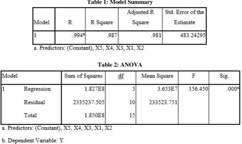
Table 1: Model Summary
Table 3: Collinearity Diagnostics
Table 3 shows evidence of multicollinearity present on the basis of Eigen values.
Table 4: Coefficients
From the above table, we can conclude that:
The VIF of X1 = 130.829 > 10 and Tolerance = .008 < 0.1 then there is multicollinearity problem at this
variable.
The VIF of X2 = 639.050 > 10 and Tolerance = .002 < .01 then there is multicollinearity problem at this
variable.
The VIF of X3 = 10.787 > 10 and Tolerance = .093 < 0.1 then there is multicollinearity problem at this variable
The VIF of X4 = 2.506 < 10 and Tolerance = .399 > 0.1 then there is no multicollinearity problem at this
variable
The VIF of X5 = 339.012 < 10 and Tolerance = .003 > 0.1 then there is multicollinearity problem at this
variable.
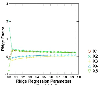
Figure 1: Ridge Trace
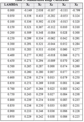
Table-5 shows the different k values under the different ridge estimators mode, it can be seen that regression coefficients is to stable with the k ridge parameter incensement. When k = .55 is accepted the corresponding fitting equation is:
Table 5: Standardized Ridge Coefficients
5. CONCLUDING REMARKS
Various methods are available in literatures for detection of multicollinearity such as examination of correlation matrix, Chi-Square test, looking pattern of eigenvalues and others. The complete elimination of multicollonearity is not possible but degree of multicollinearity present in the data may be reduced. Several remedial measures can be applied to tackle the problem of multicollinearity. But our study relates to RR only.
In our study packages like SPSS and SYSTAT are used for constructing the linear model between the dependent variable [No. of people employed, in thousands “Y”] and the explanatory variables: [GNP implicit price deflator ‘X1’, GNP, millions of dollars ‘X2’, No. of people unemployed, in thousands ‘X3’, No. of people in the armed
forces ‘X4’, Noninstitutionalized population over 14 years of age X5]. In addition, a test is applied for the
multicollinearity by extracting the VIF quantities. Therefore, a multicollinearity problem has been observed at our constructed model. The technique of RR is used to deal with the problem of multicollinearity at the constructed model. By using the SYSTAT package, all values of coefficients are estimated based on suitable values of k and estimate of the model has been discussed.
REFERENCES
[1]. Draper, N. R. (1963), “Ridge Analysis of Response Surveys”, Technometrics, 5 (4), 469 - 479.
[2]. Farrar, D. E. and Glauber, R. R. (1967), “Multicollinearity in Regression Analysis: The Problem Revisited”, the Review of Economics & Statistics, Vol. 49, pp. 92-107.
[3]. Frisch, R. (1934), “Statistical Confluence Analysis by Means of Complete Regression Systems”, Institute of Economics, Oslo University, Publication No. 5.
[5]. Hoerl, A. E. and R. W. Kennard (1970 a), “Ridge Regression: Biased Estimation of Nonorthogonal Problems”, Technometrics, 12 (1), 55-67.
[6]. Hoerl, A. E. and R. W. Kennard (1970 b), “Ridge Regression: Application to Nonorthogonal Problems”, Technometrics, 12 (1), 69-82.
[7]. Johnson, S. R., S. C. Reimer and T. P. Rothrock (1973), “Principal Components and the Problem of Multicollinearity”, Metroeconomica, 25 (3), 306 -317.
[8]. Marquardt, D. W. (1970), “Generalized Inverses, Ridge regression: Biased Linear Estimation and Non-linear Estimation”, Technometrics, Vol. 12, pp. 591 - 612.
[9]. Singh, R. (2013), “Origin of Econometrics”, International Journal of Research in Commerce, Economics & Management, published in Vol. 3 (Jan or Feb 2013).