Deep Reinforcement Learning for Drone Delivery

Article

Deep Reinforcement Learning for Drone Delivery

Guillem Muñoz, Cristina Barrado * , Ender Çetin and Esther Salami

Computer Architecture Department, UPC BarcelonaTECH, Esteve Terrades 7, 08860 Castelldefels, Spain; [email protected] (G.M.); [email protected] (E.Ç.); [email protected] (E.S.)

* Correspondence: [email protected]; Tel.: +34-934-137-208

Received: 16 August 2019; Accepted: 4 September 2019; Published: 10 September 2019

Abstract:Drones are expected to be used extensively for delivery tasks in the future. In the absence of obstacles, satellite based navigation from departure to the geo-located destination is a simple task. When obstacles are known to be in the path, pilots must build a flight plan to avoid them. However, when they are unknown, there are too many or they are in places that are not fixed positions, then to build a safe flight plan becomes very challenging. Moreover, in a weak satellite signal environment, such as indoors, under trees canopy or in urban canyons, the current drone navigation systems may fail. Artificial intelligence, a research area with increasing activity, can be used to overcome such challenges. Initially focused on robots and now mostly applied to ground vehicles, artificial intelligence begins to be used also to train drones. Reinforcement learning is the branch of artificial intelligence able to train machines. The application of reinforcement learning to drones will provide them with more intelligence, eventually converting drones in fully-autonomous machines. In this work, reinforcement learning is studied for drone delivery. As sensors, the drone only has a stereo-vision front camera, from which depth information is obtained. The drone is trained to fly to a destination in a neighborhood environment that has plenty of obstacles such as trees, cables, cars and houses. The flying area is also delimited by a geo-fence; this is a virtual (non-visible) fence that prevents the drone from entering or leaving a defined area. The drone has to avoid visible obstacles and has to reach a goal. Results show that, in comparison with the previous results, the new algorithms have better results, not only with a better reward, but also with a reduction of its variance. The second contribution is the checkpoints. They consist of saving a trained model every time a better reward is achieved. Results show how checkpoints improve the test results.

Keywords:drones; deep learning; reinforcement learning; Q-learning; DQN; JNN

1. Introduction

Drones, extensively used today in surveillance and remote sensing tasks, start to also span in delivery tasks [1–4]. For such outdoor tasks, global navigation satellite system (GNSS) is the major solution for navigation. This solution has proven to be efficient and accurate, but fails in denied GNSS environments [5]. Moreover, when obstacles in the path are unknown, there are too many of them, or they are at not fixed positions, then building a safe flight plan becomes very challenging. The same applies in environments with a weak satellite signal, such as indoors, under trees canopy or in urban canyons, where the current GNSS drone navigation may fail. Artificial intelligence, a research area with increasing activity, can be used to overcome such challenges. Initially focused on robots and now mostly applied to ground vehicles, artificial intelligence begins to also be used to train drones. Reinforcement learning (RL) is the branch of artificial intelligence able to train machines. Reinforcement learning is inspired by a human’s way of learning, based on trial and error experiences. In RL, agents are the computerized systems that learn, and the trial and error experiences are obtained by interacting with the environment. Using the information about the environment, the agent makes decisions and

makes actions in discrete intervals known as steps. Actions produce changes in the environment and also a reward. A reward is a scalar value informing about the benefit or inconvenience of such action. The objective of the agent is to maximize the final reward by learning which action is the best for each state. The application of RL will provide drones with more intelligence, eventually converting them in fully-autonomous machines.

As in [6–9], this paper applies RL to drones, but, in this paper, the focus is on drone delivery. Authors also extend RL using deep learning, usually known as deep reinforcement learning or deep learning. Deep RL proposes the use of neural networks in the decision algorithm. In conjunction with the experience replay memory, deep RL has been able to achieve a super-human level when playing video and board games [10]. Typical applications of deep RL are optimal sensorimotor control of autonomous robotic agents in immersive environments. Deep RL has been widely used also in other fields such as machine vision, optimal path finding, or parameter optimization.

This paper proposes the use of deep RL for training a drone to fly to a destination in a neighborhood environment with plenty of obstacles. The deep RL solution is based on double deep Q-network (DDQN) [11], an extension of deep Q-network [12]. Given a depth image, DDQN selects the action of the agent that maximizes the Q-value. Q-values are estimations of the future reward of an action executed in a given state. In contrast with previous work [13], where relevant scalar state information was embedded into the depth image, the solution proposed in this paper uses directly the scalars as part of the state. As a consequence, a state containing an image and several scalars is proposed. To process such a state, authors design a neural network that joins the two state parts into a unique flow. For this reason, it was named joint neural network (JNN). Results of the JNN outperform the previous results not only with a better reward, which increases 50%, but also in the reduction of the variance of the results. Other contributions include the addition of vertical actions to the drone, the addition of geo-fence in the environment to improve the safety of the drone flight, and the checkpoints, which allow for improving the training results.

This paper is structured as follows: Section 2 presents the deep reinforcement learning nomenclature and theory. Section3applies this theory to the current delivery problem, presenting the former solution and the two new architectures extending it. In Section4, results are presented and, in Section5, they are discussed. Finally, Section6summarizes the work and concludes the paper.

2. Formalization

2.1. Reinforcement Learning

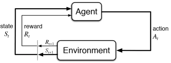
Reinforcement Learning is about learning from interaction how to behave in order to achieve a goal. The learner and decision-maker is calledagent, while the thing it interacts with, and therefore everything outside of the agent, is called theenvironment. The interaction takes place at each of a sequence of discrete time stepst. At each time step, the agent receives astate Stfrom thestate space Sand selects anaction Atfrom a set of possible actions in theaction space A(St). One time step later,

the agent gets a numericalreward Rt+1⊂Rfrom the environment as a consequence of the previous

action. Now, the agent finds itself in a new stateSt+1.

The specification of their interface defines a particular task: the actions are the choices made by the agent; the states are the basis for making choices, and the rewards are the basis for evaluating the choices. Figure1illustrates this agent-environment interaction.

At each time stept, the agent maps from states to probabilities for selecting each possible action. This mapping is called the agent’spolicyπt, withπt(a|s)as probability thatAt=aifSt=s:

Figure 1.The agent–environment interaction in reinforcement learning.

All reinforcement learning methods specify in their way how the policy is changed as a result of the agent’s experience. Informally, the goal is to choose a policy so that it maximizes the total amount of reward. This means maximizing not the immediate rewardsRt+1, but the cumulative reward over

time, called returnGt:

Gt=. Rt+1+γRt+2+γ2Rt+3+...= ∞

∑

γkRt+k+1, (2)

whereγ∈[0, 1]is thediscount factor. The discount factorγdetermines the importance of future rewards. A factor of 0 will make the agent short-sighted by only considering current rewards, while a factor approaching 1 will make it strive for a long-term high reward. Surveys of reinforcement learning and optimal control [14,15] have a good introduction to the basic concepts behind reinforcement learning used in robotics.

For reinforcement learning tasks, which break naturally into sub-sequences, calledepisodes, the return is usually left non-discounted or with a factor close to 1. Here, each episode ends in a special state called the terminal state, followed by a reset to a standard starting state. Tasks with episodes of this kind are called episodic tasks (e.g., playing chess is an episodic task with each game being one episode and checkmate as the terminal state). The discounted return is especially appropriate for continuing tasks, in which the interaction does not naturally break into episodes and continue without a limit.

2.2. Deep Q-Network

Q-learning is a well-known method for reinforcement learning when there is no knowledge of the environment or no model is available [16]. Recently, Mnih [10] was successful in combining Q-learning with neural networks and named the method deep Q-Network (DQN). The authors used DQN for learning to play Atari games and showed results of machines playing at super-human performance. The overall goal of DQN is to use a convolutional neural network (CNN) to approximate the optimal action–value function, defined as:

θπ(s,a) =max

π E

[rt+γrt+1+γ2rt+2+· · · |st=s,at=a,π]. (3)

The optimal action–value function represents the maximum of the sum of rewardsrtdiscounted

byγat each time-stept, achievable by a behaviour policyµ= P(a|s), after making an observation (s) and taking an action (a).

The release of the DQN paper by DeepMind [10] noticeably changed Q-learning introducing a novel variant with two key ideas.

The first idea was using an iterative update that adjusted the action–values (Q) towards target values (γmaxa Q(st+1,a)) that were only periodically updated, thereby reducing correlations with

The second one was using a biologically inspired mechanism named experience replay that randomizes the data removing correlations in the observations of states and enhancing data distribution, with a higher-level demonstration and explanation by previous research in [17–19]. The use of the experience replay encourages the choice of an off-policy type of learning, such as Q-learning because, if not, past experiences would have been obtained following a different policy from the current one.

Two huge advances can be taken out from this: one is that each training batch consists of samples of experience obtained randomly from the stored samples and current experience, so temporal correlation is clearly avoided. The other one is that each step in the agent’s experience can be used in many weight updates, so a significant gain in efficiency is obtained in learning from the environment.

The whole process consists of characterizing an approximate value functionQ(s,a;θi)using the

CNN shown in Equation (5), in whichθi are the weights of the Q-network at iterationi. For the

experience replay, agent’s experiencesetthat consist of the tuple(st,at,rt+1,st+1)are stored at each time-step t in the replay memorye1,· · ·,eN, where N sets the limit of entries, with the possibility of

replacing older experiences for new ones when the limit of the memory is reached.

The standard Q-learning update for network parametersθafter taking actionAtin stateStand

observing the immediate rewardRt+1and resulting stateSt+1is:

θ=θt+α[yQ_t −Q(St,At;θt)]∇θtQ(St,At;θt), (4)

where the estimated return as defined as Q-targetyQ_t :

yQ_t =Rt+1+γmax

a Q(St+1,a;θ). (5)

This update resembles stochastic gradient descent, updating the current valueQ(St,At;θt)over

the temporal difference error towards a target valueyQ_t .

2.3. Double Deep Q-Network

Using the Q-learning algorithm results in a positive bias by definition due to the maximum of the estimates is used as an estimate of the maximum of the true values, making it likely to select overestimated values using a greedy policy as the target policy. The idea proposed in [20] and named as Double Q-learning is basically based in decoupling action selection from evaluation.

Two action–value functions Q1andQ2are learned by assigning each experience randomly to update one of the two functions with the two sets of weights,θandθ0in Double Q-Learning: one set of weights is used to determine the greedy policy and the other its value:

yQ_t =Rt+1+γθ(St+1, arg max_a Q(St+1,a;θt);θt). (6)

In addition, the two Double Q-learning targets can then be written as

yDoubleQ1

t =Rt+1+γθ2(St+1, arg max_a Q1(St+1,a;θt);θ

0

t), (7)

yDoubleQ2

t =Rt+1+γθ1(St+1, arg max_a Q2(St+1,a;θ

0

t);θt). (8)

Q1is used to determine the maximizing actionA∗=arg maxaQ1(a)andQ2is used to provide the estimate of its value withQ2(A∗) =Q2(arg maxa Q1(a)) shown in Equation (7). The second set of weights can be updated symmetrically by switching the roles ofθandθ0into Equation (8), achieving unbiased estimates.

with the target network θ− a natural candidate for the second value function, without having to introduce additional networks. The DDQN algorithm remains the same as the original DQN algorithm, except replacing the targetyDQNexplained in [13] due to the limited space with

yDoubleDQN1

t =Rt+1+γθ2(St+1, arg max

a Q1(St+1,a;θt);θ −

t ), (9)

yDoubleDQN2

t =Rt+1+γθ1(St+1, arg max

a Q2(St+1,a;θ −

t );θt), (10)

where the weights of the second networkθ0of double Q-learning in Equations (7) and (8) are replaced with the weights of the target networkθ−, performing the update to target network as in neural fitted Q-iteration.

3. The Drone RL Model

In previous work [13], the authors built a deep RL solution for a drone flying in an artificial environment as shown in Figure2b. The drone had to reach a non-visible goal without crashing with any block. For this, the central part of the image was captured by the drone front camera. The image was modified to include the relative direction towards the target. Three deep Q-Learning algorithms were tested: DQN, DDQN and Dueling. The best results were obtained by DDQN. It showed to be at the level of a human tester. In this paper, DDQN is used and extended with a number of improvements.

(a) Neighbourhood (b) Blocks

Figure 2. AirSim environments with a drone and its depth camera view: (a) the new realistic environment in a neighborhood and (b) the previous work using Unreal Engine blocks [21].

Contributions of this work range from a more realistic environment to including safety considerations while smoothing the drone movements. The most relevant improvements are listed below:

1. A realistic environment: The setup of a more realistic neighborhood environment on AirSim is shown in Figure2a. It has plenty of obstacles such as trees, electric cables, houses, etc. all of them unknown to the agent.

2. Geo-fencing: Geo-fences have been added to the scenario. The geo-fencing capability is available to most drones today to help in improving safety by limiting the drone flight area. A geo-fence is a virtual barrier for the drone flight [22] and the software of the autopilot is responsible for not trespassing.

3. More degrees of freedom: The movements of the agent, a quad-copter drone, are extended from a two-dimension planar flight, at a fixed altitude, to three-dimension movements. In addition, the previous discrete action space (only two fixed speed movements and a stop action) is substituted by movements in a continuous action space, including speed variations.

5. A new neural network architecture: A DQN model is proposed in which the neural network receives a mixed state. In this mixed state, the depth image obtained by the front camera of the drone is complemented with a number of scalar values. The addition of these scalar values first reduces the size of the image and thus of the neural network model, and provides available information of the state to the agent before deciding the action. In this way, the decision model is faster and better. This neural network architecture is called a joint neural network (JNN).

3.1. Reward Function

The reward function is shown in Equation (11): a terminal step returns a reward of+100 or−100 depending on whether the episode has respectively succeeded (goal reached) or failed. Intermediate steps return a reward of−1 (to penalize delays) plus∆dg, that is, the distance-to-the-goal difference with respect to the previous step. This∆dgis used to stimulate actions that approach the goal. The only difference from the previous work is that a negative reward can be produced also in case of violation of the geo-fence. The drone must fly inside the area delimited by the geo-fence, that is, a virtual orthogonal box. The limits of the geo-fence are given by the max&min values of the box dimensions.

reward=

+100, if terminal (goal reached),

–100, if terminal (failure: obstacle or geo-fence), –1, +∆dg otherwise.

(11)

3.2. State Space

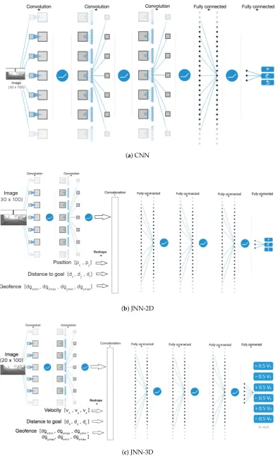
Up to three states with their respective architectures are presented and tested. For each of the three states, a different neural network has to be defined: The original convolution neural network (CNN), a first version of the joint neural network (JNN-2D) and an improved version able to manage vertical movements of the drone (JNN-3D). Each network is designed to process the three different input states.

The CNN network input is a 30×100 pixels image. The image contains the central part of the depth image (20×100 pixels) and additionally a vertical 10×10 pixel block positioned at the relative angle of the goal.

The input of the JNN-2D network is the same image, but with additional information about the state given by the following scalar values: the current location of the drone (px,pycoordinates),

the distance to the goal (dx,dy,dt, wheredt is the Euclidean distance calculated fromdx anddy),

and the distance to the geo-fence in 2D(dxmin,dxmax,dymin,dymax).

Finally, for the JNN-3D network, the image has been simplified to hold only the depth image (20×100 pixels), and the drone position is also eliminated from the state in order to avoid over-fitting. Instead, the scalar status is extended with the 3rd dimension for the geo-fence. Table 1shows a summary of the states and the neural network architectures proposed for each, wherePstands for the drone position,Gfor the distance to the goal andGFfor the distance to the geo-fence. Positions and distances are 2Din CNN and JNN-2D, and 3Dfor the JNN-3D architecture.

The three implemented networks are shown in Figure3. The CNN architecture is the one used in [10] with the updates of the input and output adequate to the drone environment. This network requires a total of 1,495,779 weights.

(a) CNN

(b) JNN-2D

(c) JNN-3D

Table 1.Summary of the three states and their neural network architectures (P stands for position of the drone, G for the goal distances and GF for the geo-fence distances).

State Double Q-Network

30×100 pixels image CNN 30×100 pixels image, P, G, GF JNN-2D 20×100 pixels image, G, GF JNN-3D

3.3. Action Space

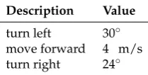
The two sets of actions are shown in Figure4. Figure 4a shows the 2D representation of the three actions in the horizontal plane. These 2D actions can be performed by going straight (4 m/s), and performing a right yaw or left yaw (30 and 24 degree angles, respectively). The new set of actions allow vertical movements of the drone, as shown in Figure4b. Let’s name ashorizontalthe former set of movements and asverticalthe new set of movements.

(a) Horizontal: 2D, discrete (b) Vertical: 3D, continuous

Figure 4.Two different action spaces.

Thehorizontalset of actions are the same three actions used in [7]. These three actions build the simplest set of actions that allow a drone to move in a fix-altitude or horizontal plane. Summary of the turn angles and the fix forward speed are shown in Table2.

Table 2.Horizontal action set.

Description Value

turn left 30◦ move forward 4 m/s turn right 24◦

The different turning angles allow up to 60 possible directions by successive turns. However, horizontalturns had the characteristic that the drone stopped before turning. This gave a swinging behaviour that should be avoided.

a stationary flight. These four images were used for the decision of the next step agent’s action. Notice that this set of actions do not include any ascending.

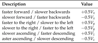
The final set ofverticalactions in three-dimensions has six possible alternatives to update the drone velocity in any one of the three axes. Each increment or decrement of the drone velocity is limited to±0.5 m/s. The complete list of actions is shown in Table3. Notice that there is no explicit action to stop the drone.

Table 3.Vertical action set.

Description Value

faster forward / slower backwards +0.5Vx slower forward / faster backwards −0.5Vx faster to the right / slower to the left +0.5Vy slower to the right / faster to the left −0.5Vy slower ascending / faster descending +0.5Vz aster ascending / slower descending −0.5Vz

3.4. Checkpoints: Improving Training Efficiency

Our training and testing environments run on a desktop with Intel i7 processor (Santa Clara, CA, USA), 16 GB of RAM and a NVIDIA GeForce GTX 1060 (Santa Clara, CA, USA) with 6 GB of RAM graphic co-processor. Since our simulation tools rely on rendering the environment which embeds the agent, each training needs around 40 h to finish.

Typically, the end of the training should result in the best model, thus the last neural network weights are stored. However, the authors have noticed that the small percent of random exploration during training leads sometimes to improve but also to worsen the model. Repeating or extending the training are too costly, and also there is no guarantee that rewards will be better. Thus, an improvement in the training process has been implemented in which the neural network weights are saved every time a best reward is obtained. These best rewards episodes are saved as checkpoints.

Now, every training creates two models: thelastmodel, containing the weights of the neural network at the end of the training, and another obtained with the last checkpoint, named asbest because it stores the neural network weights for the episode with the highest reward of the training. Tests are then executed using thelastmodel and thebestmodel and results are contrasted to show the checkpoints’ contribution.

4. Experimental Results

4.1. Setup

The environment and the drone dynamics are simulated in AirSim [23]. AirSim is a very realistic simulator, with enhanced graphics and built in scenarios. The AirSim team has published the evaluation of a quad-copter model and find that the simulated flight tracks (including time) are very close to the real-world drone behaviour.

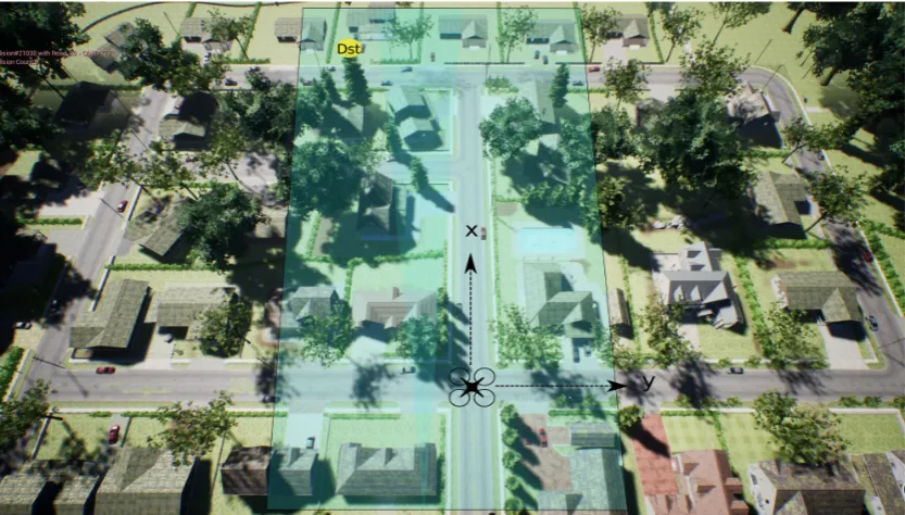
Figure 5.Two-dimensional view of the experiment setup. The drone takes off from coordinates(0, 0, 0)

and destination is set at(137,−48, 0), using thex- andy-axis shown in the image. Geo-fence highlighted in green.

After training, two different tests are executed: one to the same fixed destination (Dst) as the one trained, and two others to two alternative destinations. All destinations are located at the front of one of the houses of the neighborhood, simulating a delivery. The test to one destination consists of 100 episodes.

The parameters of the training are given in Table4. The length of the training is set to 125, 000 steps, with 50, 000 steps for thee-greedy annealing, which takes up to 42 hours of simulation to complete. The random factor of thee-greedy annealing steps decreases linearly from fully random to a 10%, and, after annealing, the random factor is kept fixed to this 10%. Replay memory, mini-batch size, target and discount factors and learning rate are fixed as in the original DDQN model of [10].

Table 4.Hyperparametres of the training.

Hyperparameter Value Observations

training steps 125, 000 annealing length 50, 000 annealing intervale [1−0.1] mini-batch size 32 replay memory 100, 000

target factorτ 0.01 frequency of the target network update discount factorγ 0.99

learning rateα 0.00025 Adam optimizer [24]

4.2. CNN Baseline Results: Checkpoint Validation

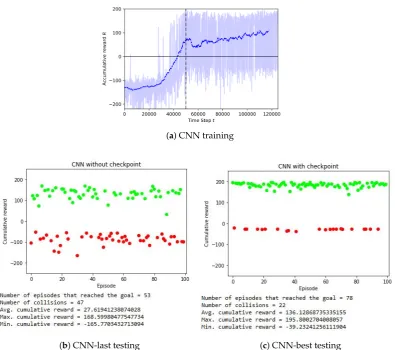
The results of the CNN model are shown in Figure6. In Figure6a, the training curve is shown: thex-axis has the steps, with a crossing line at step 50, 000 separating the annealing part from the rest. They-axis shows the reward for each consecutive episode. In light blue is the actual value of the last step of the episode, while the mean reward of 100 episodes is in dark blue.

is considered to converge and the training is finished, with the last weights of the neural network stored as the model.

Nevertheless, in cases where the oscillations are still occurring, this last value is not the best option. Checkpoints instead obtain better results as shown with the execution of one-hundred independent test episodes.

(a) CNN training

(b) CNN-last testing (c) CNN-best testing

Figure 6.Showing the benefits of checkpoints with the CNN model tests.

Results are shown in Figure6b,c, for modelinglastand modelbest, respectively, with a dot per episode. Green dots show successful episodes and red dots unsuccessful ones. They-value is the final reward of the episode. Figure6c shows the results of introducing checkpoints. Compared with Figure6b, which shows 53 episodes for which the drone was able to arrive at the destination, thebest model shows a much larger number of successful episodes (78). Moreover, the mean accumulated reward for the model resulting from the checkpoint is 136.13, greater than thelastmodel (27.62). The reason for such large differences is that the 10% of random actions used to explore the environment during training has a negative impact on the model. The checkpoint technique, by saving the neural network weights of the episode with the highest rewards, is a very good solution to balance the advantage of new explorations with the saving of knowledge. The cost of this technique is only some additional access to the disk to save the neural network weights when a new episode proves to be better than any of the previous. A threshold of the target reward can be used to reduce the number of times the model has to be saved.

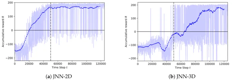
4.3. JNN Results

of each step, while the mean reward of every 100 steps is in dark blue. The vertical dotted line shows the end of the annealing training part.

(a) JNN-2D (b) JNN-3D

Figure 7.Learning curves of the three neural network architectures.

All training plots have some similar trends: observe that the first values of the reward plot are below zero, close to the crash reward value (−100). As the training proceeds and the random behaviour decreases, the trend of the reward plot starts to move up towards more positive values. After the annealing part, the models reach some stabilization, although some oscillations still appear due to the 0.1 fix randomness of the rest of the training.

By comparing the learning curves of the CNN and JNN-2D models (Figures 6a and 7a, respectively), one can observe the huge improvement of the JNN model: the learning is much faster for JNN-2D, needing only 25, 000 steps to start having many successful episodes, in contrast with the CNN model that has to wait almost double the number of steps. Moreover, the learning curve of JNN-2D stabilizes at a much higher reward value than CNN. This demonstrates that the addition of scalar information to the agent’s state is more efficient in comparison with an equivalent neural network using only the image as state. The only inconvenience is the increase of the network size, but this is a minor increase (less than 0.1%).

Then, comparing JNN-2D and JNN-3D (Figure7a,b, respectively), the JNN-3D reached almost the same reward values than the JNN-2D but in a more erratic way. The reason is that the much larger state-space, with the addition of the vertical movements, makes learning more difficult. Observe how the training curve, around the step 40, 000 gets a sequence of very low rewards (around−200). These correspond to episodes that have started to learn how to avoid obstacles and last longer, but end with a final crash or a geo-fence violation. Some of these episodes ending with very low rewards still happen close to the end of the learning. It is clear that many vertical movements do not contribute to better reach the goal. A possible reason is the flat neighborhood of the simulated scenario. Moreover, the selected flight altitude in the training and testing of the JNN-2D was below the electrical wires, which are a major problem for these low altitude flights.

Nevertheless, the flying behavior of the JNN-3D shows a notable improvement in the dynamics of the drone. Additionally, the size of the model has also decreased. While the CNN network needed to store 887, 203 weight parameters, the JNN-3D reduces them to 642, 982 thanks to the reduction of the input image size on ten rows. The scalar parameters affect only the creation of 768 new parameter weights.

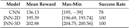
Details about the number of successful episodes, average reward and best flight reward are shown in Table5. Notice that the 3D actions obtain better rewards than the 2D model, with a higher average and higher maximum and minimum values.

(a) Test of JNN-2D (b) Test of JNN-3D

Figure 8.Comparing results of 100 test episodes using JNN-2D and JNN-3Dbestmodels.

Table 5.Model tests comparison.

Model Mean Reward Max-Min Success Rate

CNN 136.13 [195,−39] 78

JNN-2D 195.39 [196.69, 193.74] 100 JNN-3D 202.88 [204.75, 200.56] 100

4.4. Model Generalization

In order to study how well these learning models can be generalized, two new destinations were also tested. Figure9shows the environment and the drone initial position[0, 0]. Then, D1[137,−48] stands for the trained position and the test above, and D2[60,−15] and D3[137,−5]are the new destinations for these new tests. Notice that D2 is much closer to the drone initial position, and on the way to D1. It should be easy for the drone to reach this goal. The other destination, D3, is not in the same direction, but has no obstacles in the way. A priori, it seems that the drone should also be able to achieve the goal.

These tests to new destination points used thebestcheckpoint model too. Results are given in Figure10, where the left column plots show destination D2 results and the right column destination D3. There is a row per each model: CNN, JNN-2D and JNN-3D. Some of the tests show an erratic behaviour when trying to head towards the destination but were able to avoid obstacles continuously. As a pragmatic measure, a maximum time to reach the goal was set and the episode run was stopped after the given time limit. These episodes are shown in yellow in these new plots.

The tests performed to reach the second destination (D2) are shown in Figure10a,c,e for the D2 and in Table6. As it is seen in the figures, CNN and JNN-2D models have successfully reached the goal without crashing. Average cumulative rewards for CNN and JNN-2D are 133 (96% of maximum reward) and 136 (98% of maximum reward), respectively. Compared to CNN, JNN-2D has a better average reward and more smooth episodes with minimum steps possible within the environment and actions defined before. In addition, JNN-2D has higher minimum cumulative reward than CNN.

realize this and turns back to find the D2, but, most of the time, it ends up colliding with the house or the trees while searching.

In this case of the test to the destination D3, a more challenging destination is given because the heading is different from D1, and D3 is somewhere just behind the fences. The results related to the third destination (D3) can be seen in Figure10b,d,f, and numerically in Table6. The CNN model has 99 successful episodes out of 100, with only one crashed episode and an average cumulative reward of 191. In contrast, the JNN-2D and JNN-3D models have struggled to reach the destination successfully. JNN-2D reached 79 episodes and crashed 21 episodes, with an average cumulative reward of only 43. The agent earned a lower reward because it followed a route that was not leading to the destination, instead of going straight to it. The agent chose to turn slightly to the right, following a path with many obstacles, such as trees and houses. Most of the time, the agent spent its time avoiding obstacles. In the case of the JNN-3D model, no episodes reached destination D3. Results of the 100 episodes are 26 collisions and 74 episodes terminated because of the time limit, without collisions. In Figure10f, the yellow color represents the episodes that reached the time limit and the red one represents the failure episodes. The behavior of this agent is similar to an animal trying to find food at the location where it is supposed to be, but, once it realized that there is no food there, the animal searches for the food in an erratic way, by going backwards and forwards between the D1 and D3.

As a conclusion, the model generalization tests showed that the CNN model, which was not so good in reaching D1, is more generalist than the JNN models. Specifically, the model JNN-3D obtains really bad results when trying to reach a different destination than the trained one.

Figure 9.Two-dimensional view of the test experiment setup for two new destinations (D2 and D3). Geo-fence highlighted in green.

Table 6.Comparing rewards and successful rate of the three models to the different destinations.

D1 D2 D3

Model Mean Max-Min Success Mean Max-Min Success Mean Max-Min Success

CNN 136 [195,−39] 78 133 [138, 124] 100 191 [196,−16] 99

JNN-2D 195 [197, 194] 100 136 [137, 128] 100 43 [193,−186] 79

(a) CNN to D2 (b) CNN to D3

(c) JNN-2D to D2 (d) JNN-2D to D3

(e) JNN-3D to D2 (f) JNN-3D to D3

Figure 10.Test results of CNN, JNN-2D and JNN-3D for new destinations.

5. Discussion

The application of a deep RL into real life is a big challenge being addressed in research. Polvara et al. [8] used deep RL for training a drone to find and land on a landmark. A finite-state machine was in charge of switching from the initial searching phase to the next descending maneuver phase. Each phase was trained with DDQN and then tested in several scenarios with different textures. Noticeably, the trained agent was also tested in a real environment, although the success rate dropped from around 90% of the simulations to 50–60% in the real world. The limited modeling capacity of the simulator used, Gazebo 7 with ROS (OSRF, Mountain View, CA, USA), impeded the training in extreme conditions (changing of lighting and strong drift) that were found in the real world and caused most of the failures.

the Roboschool [26], the discrete and continuous control environments of MuJoCo’s [27] and the Olympic sport simulator (curling) [28].

Using neural networks (but not RL), an interesting experiment was conducted with drones directly in a real-life environment [7]. A low cost drone with three cameras and protected blades was launched to fly indoors to create a dataset of crashes. The authors used the ImageNet classification CNN [29], extended it with three more layers (dense), and used the crash data for self-training the drone’s flight policy. No vertical movements were considered. Although rewards were not part of the algorithm, the goal was to maximize the flight time and distance as long as possible, avoiding spinning loops.

In addition, not using RL, other real life experiments are published, but targeting robotic arms and self-driving cars. For instance, a set of robotic arms was monitored with an external camera to learn to grasp objects from a front tray [30]. Although no reward was involved, a deep neural network was used to derive the probabilities of success out of a number of actions. The neural network consisted of two joint input streams: The first stream involved two images of the robotic arm, the image at time 0 and the last obtained image. This first stream was processed by a five-layered CNN. The second stream had an input vector with five elements which contained the commanded movements of the arm. This vector was processed in a fully connected layer, replicated, tilled and point-wise added with the first stream output. The resulting matrix went through 13 more layers, the last two being dense.

Other research also using DQN in optimal control has shown successful results by simulation. For instance, in [31], it exploited DQN to find the optimal path of a robotic agent in a simple 2D environment with a limited number of states and no uncertainties (a 15×15 grid). DQN was also used for path planning of a ground robot in theseekavoid arena 01, a virtual environment on the DeepMind Lab platform containing some visual obstacles [32]. Another extension of DQN [33] showed a speeding-up of the learning process. The authors proposed a neural episodic control that consisted basically of adding to the experience replay a new look-up layer, in the form of an append-only memory. The objective was to detect the context of the state in the selection of the mini-batch.

This paper presents a variant of DQN too. It consists of a joint neural network, named JNN. JNN joins two different parts of the state: the image obtained from the front camera of the drone, and some complementary information in the form of scalar values. The addition of these scalars has been shown to improve the results in the trained destination compared to the image-only state, both in terms of mean reward values and in the time to reach the destination.

A limited number of research works present architectures similar to JNN. Although they also combined scalar and image inputs in a neural network, this was never used for the RL state. For instance, in the hybrid reward architecture of [34], the authors built separate value functions by decomposing the reward in different items. Then, they trained each network separately, for each one of the reward items. The final action was decided according to the aggregated values. This solution demonstrated obtaining faster convergence, but used separated neural networks. In [35], a decomposition of the neural network into two streams was tested among four different environments, including a driving simulator in an urban environment. The two streams were one to estimate the linear control and another for the nonlinear. Again, the training was not joint in a unique neural network. The most similar architecture to the JNN model presented in this paper is proposed in [36], but it is applied to supervised learning, not in reinforcement learning. The three inputs are: one image, some scalar measurements and the goal. The image is processed by a CNN. The scalar and goal inputs are processed in parallel in two dense networks. The outputs of the three independent networks are then joint as one vector state J.

6. Conclusions

In addition, the drone actions space were more realistic by including continuous movements in the three-dimensional space.

Additionally to the above, the main contributions of the paper have been the proposal of a neural network architecture joining images and scalars as part of the state, and the enhancement in the training results with the checkpoint concept. The addition of the scalar information into the agent’s state has proven to be more efficient in comparison with an equivalent neural network using only the image as state. The proposed joint neural network, which was named JNN, successfully outperformed CNN with better rewards and by reducing the variance of the results. Variability reduction is a much desired characteristic for the air traffic management and airspace safety. Moreover, the convergence of JNN is much faster compared with CNN.

Artificial intelligence is still developing and this research has opened some challenges. For instance, the time of the agent’s training is a limitation, but speed can be increased, for instance by avoiding the fully rendering. In addition, training speed can be improved by using transfer learning. With transfer learning, each new training starts with an already trained model. This helps to extend the training with new challenges, such as new destinations. It is clear that, for delivery tasks, the current model shall be improved to obtain a more generalist model, able to reach goals at any location.

Another challenge is the training of multiple agents using deep RL. Luckily, the AirSim new version has incorporated the multi-agent capability that opens the door to the extension of this work with it. To conclude, for the validation of the trained models in the real world, using drones is the final target.

Author Contributions:Conceptualization, C.B. and E.S.; methodology, G.M.; software, G.M. and E.Ç.; validation, G.M., C.B. and E.S.; writing, G.M. and C.B.

Funding:This work was funded by the Ministry of Science, Innovation and Universities of Spain under Grant No. TRA2016-77012-R.

Acknowledgments: The authors acknowledge the initial setup by Kjell Kersandt and the help given by Francesc Tarres.

Conflicts of Interest:The authors declare no conflict of interest.

References

1. Hii, M.S.Y.; Courtney, P.; Royall, P.G. An Evaluation of the Delivery of Medicines Using Drones. Drones 2019,3, 52. [CrossRef]

2. Yoo, W.; Yu, E.; Jung, J. Drone delivery: Factors affecting the public’s attitude and intention to adopt.

Telemat. Informat.2018,35, 1687–1700. [CrossRef]

3. Dorling, K.; Heinrichs, J.; Messier, G.G.; Magierowski, S. Vehicle routing problems for drone delivery.

IEEE Trans. Syst. Man Cybern. Syst.2016,47, 70–85. [CrossRef]

4. Bamburry, D. Drones: Designed for product delivery.Des. Manag. Rev.2015,26, 40–48.

5. Altawy, R.; Youssef, A.M. Security, privacy, and safety aspects of civilian drones: A survey. ACM Trans. Cyber-Phys. Syst.2017,1, 7. [CrossRef]

6. Akhloufi, M.A.; Arola, S.; Bonnet, A. Drones Chasing Drones: Reinforcement Learning and Deep Search Area Proposal.Drones2019,3, 58. [CrossRef]

7. Gandhi, D.; Pinto, L.; Gupta, A. Learning to fly by crashing. In Proceedings of the 2017 IEEE/RSJ International Conference on Intelligent Robots and Systems (IROS), Vancouver, BC, Canada, 24–28 September 2017; pp. 3948–3955.

8. Polvara, R.; Patacchiola, M.; Sharma, S.; Wan, J.; Manning, A.; Sutton, R.; Cangelosi, A. Autonomous Quadrotor Landing using Deep Reinforcement Learning.arXiv2017, arXiv:1709.03339.

9. Chowdhury, M.M.U.; Erden, F.; Guvenc, I. RSS-Based Q-Learning for Indoor UAV Navigation. arXiv2019, arXiv:1905.13406.

10. Mnih, V.; Kavukcuoglu, K.; Silver, D.; Rusu, A.A.; Veness, J.; Bellemare, M.G.; Graves, A.; Riedmiller, M.; Fidjeland, A.K.; Ostrovski, G.; et al. Human-level control through deep reinforcement learning.Nature2015,

11. Van Hasselt, H.; Guez, A.; Silver, D. Deep Reinforcement Learning with Double Q-Learning; AAAI: Phoenix, AZ, USA, 2016; Volume 2, p. 5.

12. Mnih, V.; Kavukcuoglu, K.; Silver, D.; Graves, A.; Antonoglou, I.; Wierstra, D.; Riedmiller, M. Playing atari with deep reinforcement learning.arXiv2013, arXiv:1312.5602.

13. Kersandt, K.; Muñoz, G.; Barrado, C. Self-training by Reinforcement Learning for Full-autonomous Drones of the Future. In Proceedings of the 2018 IEEE/AIAA 37th Digital Avionics Systems Conference (DASC), London, UK, 23–27 September 2018; pp. 1–10.

14. Kiumarsi, B.; Vamvoudakis, K.G.; Modares, H.; Lewis, F.L. Optimal and autonomous control using reinforcement learning: A survey. IEEE Trans. Neural Netw. Learn. Syst. 2018,29, 2042–2062. [CrossRef] [PubMed]

15. Sutton, R.S.; Barto, A.G.Reinforcement Learning: An Introduction; MIT Press: Cambridge, UK, 1998. 16. Watkins, C.J.; Dayan, P. Q-learning.Mach. Learn.1992,8, 279–292. [CrossRef]

17. McClelland, J.L.; McNaughton, B.L.; O’Reilly, R.C. Why there are complementary learning systems in the hippocampus and neocortex: Insights from the successes and failures of connectionist models of learning and memory. Psychol. Rev.1995,102, 419–457, doi:10.1037/0033-295X.102.3.419. [CrossRef] [PubMed] 18. Riedmiller, M.Neural Fitted Q Iteration-First, Experiences with a Data Efficient Neural Reinforcement Learning

Method; ECML; Springer, Berlin, Heidelberg, Germany, 2005; Volume 3720, pp. 317–328.

19. Lin, L.J. Reinforcement Learning for Robots Using Neural Networks. Ph.D. Thesis, Carnegie-Mellon Univ, School of Computer Science, Pittsburgh, PA, USA, January 1993.

20. Hasselt, H.V. Double Q-learning. In Proceedings of the Advances in Neural Information Processing Systems (NIPS), Vancouver, BC, Canada, 6–11 December 2010; pp. 2613–2621.

21. Unreal Engine 4. Available online: https://www.unrealengine.com/en-US/what-is-unreal-engine-4

(accessed on 29 January 2019).

22. Dasu, T.; Kanza, Y.; Srivastava, D. Geofences in the Sky: Herding Drones with Blockchains and 5G. In Proceedings of the 26th ACM SIGSPATIAL International Conference on Advances in Geographic Information Systems, Seattle, WA, USA, 6–9 November 2018; doi:10.1145/3274895.3274914. [CrossRef] 23. Shah, S.; Dey, D.; Lovett, C.; Kapoor, A. AirSim: High-Fidelity Visual and Physical Simulation for

Autonomous Vehicles.arXiv2017, arXiv:1705.05065.

24. Kingma, D.P.; Ba, J.L. Adam: Amethod for stochastic optimization. arXiv2014, arXiv:1412.6980.

25. Bellemare, M.G.; Naddaf, Y.; Veness, J.; Bowling, M. The arcade learning environment: An evaluation platform for general agents. J. Artif. Intell. Res.2013,47, 253–279. [CrossRef]

26. Brockman, G.; Cheung, V.; Pettersson, L.; Schneider, J.; Schulman, J.; Tang, J.; Zaremba, W. Openai gym.

arXiv2016, arXiv:1606.01540.

27. Chou, P.W.; Maturana, D.; Scherer, S. Improving Stochastic Policy Gradients in Continuous Control with Deep Reinforcement Learning using the Beta Distribution. In Proceedings of the ICML’17 Proceedings of the 34th International Conference on Machine Learning, Sydney, Australia, 6–11 August 2017; Precup, D., Teh, Y.W., Eds.; PMLR International Convention Centre: Sydney, Australia, 2017; Volume 70, pp. 834–843. 28. Lee, K.; Kim, S.A.; Choi, J.; Lee, S.W. Deep Reinforcement Learning in Continuous Action Spaces: A Case

Study in the Game of Simulated Curling. In Proceedings of the 35th International Conference on Machine Learning (ICML), Stockholm, Sweden, 10–15 July 2018; pp. 2943–2952.

29. Girshick, R.; Donahue, J.; Darrell, T.; Malik, J. Rich feature hierarchies for accurate object detection and semantic segmentation. In Proceedings of the IEEE Conference on Computer Vision and Pattern Recognition, Columbus, OH, USA, 24–27 June 2014; pp. 580–587.

30. Levine, S.; Pastor, P.; Krizhevsky, A.; Ibarz, J.; Quillen, D. Learning hand-eye coordination for robotic grasping with deep learning and large-scale data collection.Int. J. Robot. Res.2018,37, 421–436. [CrossRef] 31. Bai, X.; Niu, W.; Liu, J.; Gao, X.; Xiang, Y.; Liu, J. Adversarial Examples Construction Towards White-Box Q Table Variation in DQN Pathfinding Training. In Proceedings of the 2018 IEEE Third International Conference on Data Science in Cyberspace (DSC), Guangzhou, China, 18–21 June 2018.

33. Pritzel, A.; Uria, B.; Srinivasan, S.; Badia, A.P.; Vinyals, O.; Hassabis, D.; Wierstra, D.; Blundell, C. Neural Episodic Control. In Proceedings of the 34th International Conference on Machine Learning, Sydney, Australia, 6–11 August 2017; Precup, D., Teh, Y.W., Eds.; PMLR International Convention Centre: Sydney, Australia, 2017; Volume 70, pp. 2827–2836.

34. Van Seijen, H.; Fatemi, M.; Romoff, J.; Laroche, R.; Barnes, T.; Tsang, J. Hybrid Reward Architecture for Reinforcement Learning. In Proceedings of the Advances in Neural Information Processing Systems 30, Long Beach, CA, USA, 4–9 December 2017; pp. 5392–5402.

35. Srouji, M.; Zhang, J.; Salakhutdinov, R. Structured Control Nets for Deep Reinforcement Learning. In Proceedings of the 35th International Conference on Machine Learning, Stockholm, Sweden, 10–15 July 2018; Dy, J., Krause, A., Eds.; PMLR Stockholmsmässan: Stockholm Sweden, 2018; Volume 80, pp. 4749–4758. 36. Dosovitskiy, A.; Koltun, V. Learning to act by predicting the future. arXiv2016, arXiv:1611.01779.

c